Realistic protein–protein association rates from a simple diffusional model neglecting long-range interactions, free energy barriers, and landscape ruggedness

Abstract

We develop a simple but rigorous model of protein–protein association kinetics based on diffusional association on free energy landscapes obtained by sampling configurations within and surrounding the native complex binding funnels. Guided by results obtained on exactly solvable model problems, we transform the problem of diffusion in a potential into free diffusion in the presence of an absorbing zone spanning the entrance to the binding funnel. The free diffusion problem is solved using a recently derived analytic expression for the rate of association of asymmetrically oriented molecules. Despite the required high steric specificity and the absence of long-range attractive interactions, the computed rates are typically on the order of 10⁴–10⁶ M⁻¹ sec⁻¹, several orders of magnitude higher than rates obtained using a purely probabilistic model in which the association rate for free diffusion of uniformly reactive molecules is multiplied by the probability of a correct alignment of the two partners in a random collision. As the association rates of many protein–protein complexes are also in the 10⁵–10⁶ M⁻¹ sec⁻¹ range, our results suggest that free energy barriers arising from desolvation and/or side-chain freezing during complex formation or increased ruggedness within the binding funnel, which are completely neglected in our simple diffusional model, do not contribute significantly to the dynamics of protein–protein association. The transparent physical interpretation of our approach that computes association rates directly from the size and geometry of protein–protein binding funnels makes it a useful complement to Brownian dynamics simulations.

The calculation of rates of protein–protein association is of great interest to biology. These rates span a wide range of values, from ~10³ to 10¹⁰ M⁻¹ sec⁻¹. If the two proteins are modeled as uniformly reactive spheres, the diffusion-limited rate constant is simply given by the classical Smoluchowski expression (Smoluchowski 1917), k_on = 4πDR (where D is the relative translational diffusion constant and R is the sum of the radii), which yields rates of 10⁹–10¹⁰ M⁻¹ sec⁻¹ for associations relevant to proteins. Usually, however, proteins exhibit a highly anisotropic distribution of reactivity over their surface. This can be modeled by localized reactive sites on the surface of the proteins that have to be sufficiently precisely aligned for the complex formation to occur.

Purely probabilistic models have tried to account for such steric constraints by multiplying the Smoluchowski rate for uniform spheres by the probability that, in a random encounter, the two molecules are properly aligned (“geometric rate”; Janin 1997 gives an example of this method). This yields rate constants that are typically several orders of magnitude lower than the Smoluchowski diffusion-limited rate and are usually much smaller than the values experimentally observed for biological complexes. It has been found that this discrepancy can be moderated by taking into account the effect of rotational diffusion (Shoup et al. 1981; Northrup and Erickson 1992); additional rate enhancements are brought about by the presence of attractive interparticle forces (“electrostatic steering”; see Schreiber and Fersht 1996; Gabdoulline and Wade 1997; Vijayakumar et al. 1998), and the formation of a weakly specific, loosely bound encounter complex that subsequently evolves into the final bound state (Selzer and Schreiber 1999; Camacho et al. 2000).

To replace the estimation of protein–protein association rates via the geometric rate by a more accurate method, most authors have pursued a computational approach by carrying out explicit numerical simulations of the diffusional association of macromolecules, commonly referred to as Brownian dynamics (BD) simulations (for an excellent review, see Gabdoulline and Wade 2002). Here, the protein molecules are modeled in varying detail, from a simple spherical approximation up to full atomic detail. In the simulation, the molecules are initially placed in random orientations at a fixed initial separation b. Diffusional trajectories, with or without the presence of an interparticle force (such as electrostatic interactions), are then generated by means of the Ermak–McCammon algorithm (Ermak and McCammon 1978). A trajectory is ended either when the molecules have come together in proper orientation to successfully form a complex, or when their separation has exceeded a certain truncation value c > b such that the probability for an encounter has become vanishingly small. The fraction of “successful” trajectories is then used to compute the association rate k_on.

Northrup and Erickson (1992) have used such a BD simulation to compute the association rate of spherical molecules with a reactive patch, consisting of four contact points in a 17 Å × 17 Å square arrangement on a plane tangential to the surface of the molecules. A reaction is then assumed to occur if three of the four contact points are correctly matched and within a specified maximum distance. In the absence of any interparticle forces, the authors find an association rate of k_on = 10⁵ M⁻¹ sec⁻¹, about two orders of magnitude higher than the geometric rate. Gabdoulline and Wade (2001) compute association rates for five protein–protein complexes using full-atom structures in the presence of long-range electrostatic forces. The reaction condition is defined by formation of subsets of the polar contacts observed in the native complex structure.

In this paper, we present a different route toward estimation of rates of bimolecular association. Instead of using a computer-simulation-based approach such as the method of BD simulations outlined above, we use a recently derived analytical expression (Schlosshauer and Baker 2002) for the association rate of two spherical molecules with anisotropic reactivity in the absence of any interaction forces. The reaction condition is formulated by specifying the ranges of mutual orientations of the two molecules for which complex formation will occur. We thus do not require an exact mutual alignment of the binding partners, but instead assume that favorable short-range interactions “guide” the molecules into their final bound configurations once the molecules are oriented within specified angular tolerances (see Fig. 1 ▶). These tolerances can therefore be viewed as an implicit modeling of attractive short-range forces. We derive estimates for the tolerances from free energy landscapes obtained by sampling configurations within and surrounding the native binding funnel. These values are then used in our analytical expression to compute the corresponding association rates. By determining the size and geometry of the aperture in phase space that must be entered for binding to occur, and rigorously solving the problem of diffusion through this aperture, our approach provides a physically transparent complement to BD simulations for computing binding rates from structures of protein–protein complexes.

Figure 1.

Simple model of binding dynamics. Attractive short-range forces produce a funnel in the free energy landscape leading into the native complex. Once the molecules descend several kT into the funnel, they are effectively captured and binding occurs rapidly. In our simple model, the rate of association is approximated by the rate of free diffusion into a reactive zone in phase space, as indicated schematically in the XY plane of the drawing. To compute the rate of association, we need first to determine the dimensions of the reactive zone, and second, to compute the rate of free diffusion into this zone. A more general model would include long-range (electrostatic) interactions that would bias the diffusion process toward the funnel entrance.

Results

To compute protein–protein association rates from the three-dimensional (3D) structures of protein–protein complexes according to the simple diffusive model described above and in Figure 1 ▶, three ingredients are required. The first is a general theory for computing the diffusion-limited association rate as a function of the orientational constraints associated with properly aligning the two binding sites (the size and shape of the reactive zone in Fig. 1 ▶). The second is a method for transforming a diffusion in a potential problem into a free diffusion problem—in the context of Figure 1 ▶, an estimate of how deeply the reactive zone lies within the binding funnel (i.e., how far molecules must descend into the binding funnel before they are effectively captured). The third is a method for mapping the binding funnel for two proteins given the crystal structure of the protein–protein complex. We address these issues in the next three sections and then, in the fourth section, use the results to compute approximate diffusion limited association rates from the structures of protein–protein complexes.

Theory for the diffusion-limited association rate with general orientational constraints

Here, we restrict ourselves to a brief outline; the full derivation of our expression for the association rate constant in the presence of general orientational constraints can be found in Schlosshauer and Baker (2002).

We consider translational and rotational diffusional motion of two spherical molecules A nd B with radii R_A and R_B. To derive an expression for the association rate constant, we solve the steady-state translational–rotational diffusion equation describing the diffusional motion of the two spheres, subject to a reaction condition that ensures that binding can only occur if the mutual orientation of the two spheres is sufficiently close to the orientation in the bound configuration that defines the optimal alignment.

The reaction condition is implemented as follows (see Fig. 2 ▶): The centers of “reactive patches” on the two spheres are defined by the intersection of the center-to-center vector with the surfaces of the spheres in the native bound configuration. Each sphere carries its own body-fixed coordinate system {x_s, y_s, z_s}, s = A, B, where the z_s axis points at the center of the reactive patch. The angles θ_A and θ_B then quantify the distance of the center of each reactive patch to the center-to-center vector, whereas the Euler angles δφ and δχ denote relative torsional angles between the body-fixed coordinate systems (x_A, y_A, z_A) and (x_B, y_B, z_B).

Figure 2.

The axes and angles relevant to the reaction condition, equation 1. The angles θ_A and θ_B measure how close the center of each reactive patch (coinciding with the respective body-fixed z-axis) is to the center-to-center vector (dashed line). The Euler angles δφ and δχ denote relative torsion angles of the two body-fixed coordinate systems (x_A, y_A, z_A) and (x_B, y_B, z_B). For the sake of easier visualization of these two angles, the origin of the x_A and y_A axes (belonging to the coordinate system of sphere A) has been shifted such as to coincide with the origin of the coordinate system of sphere B. Our reaction condition, equation 1, requires near-optimal alignment; that is, all angles θ_A, θ_B, δφ, and δχ must be below given limits.

At a first glance, one might assume that a fifth parameter is required to fully describe the mutual orientation of the two spheres—namely, an azimuthal angle φ_A in addition to the polar angle θ_A to fix the location of the reactive patch on the surface of sphere A. For the formulation of the reaction condition, however, four angles suffice, because the position of the center of the reactive patch is automatically specified through its coincidence with the z_A axis. This leaves only one free parameter, namely, the “width” of the patch, which is described by the angle θ_A.

The optimal alignment is then defined by θ_A = θ_B = δφ = δχ = 0 (additionally, the length r of the center-to-center vector must be equal to the sum of the radii of the spheres). Our reaction condition requires that all these angles are sufficiently close to zero for the reaction to occur; that is, the following conditions are fulfilled:

(1)

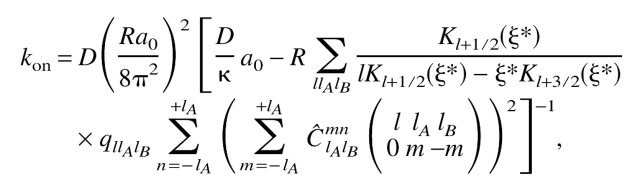
Using the constant-flux approximation introduced by Shoup et al. (1981), we obtain for the association rate constant (Schlosshauer and Baker 2002):

(2)

where D = D^trans_A + D^trans_B is the (relative) translational diffusion constant, a₀ = (4π)³δφ₀δχ0(1 − cos φ⁰_A)(1 − cos φ⁰_B), q_llAlB = (2l + 1)(2l_A + 1)(2l_B + 1)/16π³, and κ quantifies the extent of diffusion control in the reaction. Furthermore,

where d^l_mn(θ) denotes the Wigner rotation function. is the Wigner 3-j symbol, and ξ* = R[(D^rot_A /D)l_A(l_A + 1) + (D^rot_B /D)l_B(l_B + 1)]^1/2, where D^rot_A and D^rot_B are the rotational diffusion constants. â₀ = a₀/(4π × 8π² × 8π²) represents the fraction of angular orientational space over which the reaction can occur, and the geometric rate is thus given by k_on = 4πDR × â₀.

Transformation of the diffusion in a potential problem into a free diffusion problem

A crucial point in the application of equation 2 is the estimation of the angular constraints θ⁰_A, θ⁰_B, δφ₀, and δχ₀. We would like to estimate the ranges in mutual orientation of the two proteins for which short-range attractive forces between the atoms are sufficiently dominant to guide the two molecules into the final bound configuration, and then translate the problem of diffusional association in the attractive potential into free diffusion with an absorbing region in configurational space. To motivate this mapping, we first study two simple toy models for translational and rotational diffusion, respectively. We then use these ideas to explicitly obtain the angular constraints for real protein–protein complexes.

Toy model for translational diffusion

The reaction rate for diffusion-controlled bimolecular association of uniformly reactive spheres in the presence of a potential U(r) can be calculated exactly and is given by the expression

(3)

where β ≡ 1/kT, and R₁ is interpreted as the center-to-center distance between the associating partners at which the reaction is assumed to occur. Equation 3 is the classical result derived by Debye (1942). In the absence of any potential (U ≡ 0), this simplifies to the Smulochowski rate constant for free diffusion with an absorbing region of width R₀, given by k⁽⁰⁾_on = 4πDR₀ (in the following we use the label “0” to refer to the free diffusion problem, and the label “1” to refer to the diffusion in a potential problem).

It is clear that for R₀ = R₁, k⁽¹⁾_on > k⁽⁰⁾_on because the presence of the (attractive) potential will increase the association rate. To find the free diffusion analog of diffusional association in an attractive potential, we increase R₀ until k⁽⁰⁾_on > k⁽¹⁾_on. In other words, for a given potential, we can determine the size of the absorbing region (the “capture radius”) required in the case of free diffusion to obtain an association rate equivalent to that of diffusion in the potential. A similar redefinition of the effective absorbing radius to account for the presence of the potential was first introduced by Debye (1942).

A concrete illustration of this procedure is described in Figure 3 ▶ for a Lennard–Jones potential. For a broad range of parameter values, we find that it is sufficient to drop down by an energy amount of only 𝒪(ΔE) = kT to enter the capture zone, corresponding to <5% of the total depth of the potential. The capture radius R₀ is found to be relatively insensitive to the depth ɛ of the potential well, whereas its dependence on the width σ is much stronger—as it must be, because R₀ is an indirect measure of the range of the potential.

Figure 3.

Mapping of translational diffusional association in a short-range attractive potential onto the problem of free diffusion with an absorbing region. A Lennard–Jones potential with parameters appropriate to protein–protein association (ɛ = 10 kcal/mole, σ = 3 Å, R₁ = 40 Å) is shown in the figure, together with the corresponding free diffusion “capture radius” R₀. The capture radius is defined as the radius for which the free diffusion rate k_on⁽⁰⁾ is equal to the association rate in the presence of U(r), k_on⁽¹⁾. Evaluating U(r) at the capture radius yields the energy drop ΔE ≡ U(∞) − U(R₀) ≈ 0.3 kcal/mole (i.e., of order kT); this is quite insensitive to large changes in ɛ and σ.

The model calculations show that the effect of an attractive potential U(r) on the association rate can be effectively represented by an increase in the radius of the interacting spheres, but that in the relevant case of protein–protein interactions, the relative increase is very small (~7% in our example). Because the association rate (equation 2) is largely insensitive to small changes in the value of R, we conclude that the approximation of using a fixed value r = R_A + R_B ≡ R for the center-to-center distance of the two proteins required for the reaction to occur (see our reaction condition, equation 1), rather than using a range of allowed values (such as demanding that r ≤ R_A + R_B + δR [in equation 1]), is not unreasonable.

Toy model for rotational diffusion

As another illustration of our mapping procedure, we consider two-dimensional (2D) rotational diffusion on a spherical surface in an attractive Gaussian potential U(θ) = −ɛ exp[−(σ θ)²], with ɛ > 0. Again, we would like to translate this problem into that of free rotational diffusion with an absorbing region at θ = θ₀.

Solving the rotational diffusion equation in the presence of a potential U(θ) yields in the diffusion-controlled limit

(4)

where we let θ₁ → 0 for U ≢ 0 (diffusion in potential). In the case of free diffusion (U ≡ 0), equation 4 becomes:

(5)

where we now choose θ₀ > 0. As before, we equate the association rates, equations 4 and 5, to obtain an estimate for the width θ₀ of the absorbing region.

For a range of parameter values, we again find that an energy drop of ΔE ≡ U(π) − U(θ₀) of the order of kT suffices to enter the capture zone (Fig. 4 ▶). We find that θ₀ is insensitive to the choice of ɛ but increases as expected with increasing σ: The range of the absorbing region reflects the range of the potential.

Figure 4.

Mapping of the problem of diffusion in a potential onto that of free diffusion with an absorbing region for rotational diffusion on a spherical surface. We use an attractive Gaussian potential U(θ) = −ɛ exp[−(σ θ)²] with ɛ = 10 kcal/mole and σ = π, where the latter corresponds to a (half) width of the potential of , a reasonable assumption for a short-range potential. Equating the resulting association rate (equation 4) with the rate for free diffusion in the presence of an absorbing region at θ = θ ₀ (equation 5), we obtain θ ₀ ≈ 33° for the width of the absorbing region, corresponding to an energy drop of ΔE ≡ U(π) − U(θ ₀) ≈ 0.4 kcal/mole.

Discussion of the toy model results

The analysis of the toy models demonstrates that translational and rotational diffusional association in a short-range potential (as it occurs in protein–protein complex formation when the two proteins are close to each other) can be modeled as free diffusion in the presence of absorbing regions of suitably chosen size. The size of the absorbing regions is relatively insensitive to the precise shape (that is, the functional form) and magnitude of the chosen potential function; only the range of the potential must be chosen roughly right in estimating the angular constraints. The energy drop itself required to enter the capture zone (binding funnel) is found to be robust toward changes in the shape, depth, and range of the potential, and can therefore be regarded as an essentially universal quantity that is largely independent of the particular form of the interaction potential used in the mapping problem.

Because our toy models have only a one-dimensional (1D) reaction condition—that is, a constraint on a single degree of freedom—the question arises to what extent the relative influence of the potential on the reaction rate would change in the case of higher-dimensional reaction conditions (as used in our subsequent treatment of protein–protein interactions where we impose constraints on r, θ_A,B, δφ, and δχ). The results obtained by Zhou (1997) suggest that the influence of the interaction potential on the association rate constant is more significant for the case of two diffusing spheres bearing a circular reactive patch on each surface (i.e., where a 2D reaction condition is used for both spheres) than for the situation in which one of the spheres is taken to be uniformly reactive (i.e., where a 2D reaction condition is imposed on one sphere, but only a 1D reaction condition is used for the second sphere). Generalizing these findings, we may anticipate that an attractive interaction potential will affect reaction rates to a larger extent when the number of constrained variables in the reaction condition is increased. Because our toy models have shown that it suffices to enter the potential well by a relatively small amount to be “captured,” we can conclude that for the case of a higher-dimensional reaction condition as considered in the following, an even smaller energy drop will be sufficient to enter the capture zone. From the point of view of transition state theory, our approach corresponds to identifying the transition region and then computing the flux into this region.

Mapping the protein–protein interaction funnel from the structure of a protein–protein complex

Now we apply the idea outlined above to an estimate of the angular constraints θ⁰_A, θ⁰_B, δφ₀, and δχ₀, needed for the application of our expression for the rate constant, equation 2. For this purpose, we have directly taken the 3D structures of the considered complexes from the Protein Data Bank (PDB).

First, the side chains of the native complexed structure were repacked by minimizing a full-atom energy function ℰ dominated by Lennard–Jones interactions, an orientation-dependent hydrogen-bond potential, and an implicit solvation model (Gray et al. 2003). As with all current potential functions for macromolecules, there are likely to be considerable inaccuracies in this model, but it should be emphasized that the angular constraints and rates computed here are relatively insensitive to the details of the interactions—the toy examples clearly demonstrate that once the binding funnel has been entered (which has been found to require only a small drop down in energy), the detailed form of the interaction potential has only little influence.

Second, a set of 1000 alternative structures was generated from the native complex by performing random small perturbative movements around the native conformation, and the interaction energy of these structures was evaluated using the same energy function ℰ as used in the repacking procedure. The energy landscapes defined by these alternative structures exhibit clear funnels around the native minimum.

The toy model calculations show that diffusion in such landscapes can be modeled as free diffusion with an effective “capture” region several kT into the energy funnels. To define the capture energy cutoff ℰ_c below which the partners are committed to bind, we compute the average ℰ_av of the energies of the five lowest-lying structures >10 Å root mean square deviation (rmsd) from the native complex (and hence outside of the native energy funnel). Because the energy cutoff cannot be determined exactly, we obtain two different estimates of the association rate setting ℰ_c to either ℰ_av or ℰ_av − 5kT. We selected the 10 structures with the largest values of θ⁰_A + θ⁰_B in the set of structures with ℰ < ℰ_c and took the averages of their values of θ⁰_A, θ⁰_B, δφ₀, and δχ₀ to obtain estimates for the angular tolerances used in computing the association rates.

An example is shown in Figure 5 ▶. We see that the funnel-like dependence of the energy on the rmsd and on the angular deviations is akin to the shape of the attractive potentials used in the toy models for translational and rotational diffusion discussed above. Furthermore, the location of the angular constraints resembles the position of the absorbing regions of the toy models. These similarities support our approach of deriving the angular constraints θ⁰_A, θ⁰_B, δφ₀, and δχ₀ from the interaction energy of perturbed protein complex structures in general, and from our method of choosing suitable energy cutoffs in particular.

Figure 5.

Free energy funnels around the native structure. The energy ℰ and rmsd (A), the energy ℰ and the angular deviations θ_A⁰ (B), and δχ₀ (C) are shown for a set of randomly perturbed structures of the protein–protein complex 1FIN. States of lower energy are seen to be associated with smaller angles, suggesting that the angles are a reasonable measure for the deviation from the correctly complexed structure. The two parallel lines represent the two energy cutoffs ℰ_c = ℰ_av and ℰ_c = ℰ_av − 5kT, where ℰ_av is the average energy of the five lowest energy complexes with an rmsd above 10 Å. The vertical lines in the plots indicate the resulting angular constraints θ_A⁰ and δχ₀ corresponding to ℰ_c = ℰ_av (dashed line) and ℰ_c = ℰ_av − 5kT (dotted/dashed line).

Computation of diffusion-limited association rates from structures of protein–protein complexes

With the angular constraints determined as described in the preceding section, we use equation 2 in the fully diffusion-limited limit (κ → ∞) to compute protein–protein association rates. The effective radii R_A and R_B of the spheres representing the proteins are taken to be equal to the radius of gyration, R_g = (1/N)∑_id_i (where N is the number of atoms in the protein and d_i is the distance of the i-th atom from the geometric center of the protein), multiplied by a correction factor of (5/3)^1/2 to obtain the desired result R_g = R_s for the limiting case of a homogeneous sphere of radius R_s. The sum R_A + R_B is used as the value for the distance R between the centers of the two proteins at which reaction is assumed to occur; compare with equation 1. The study of our toy model for translational diffusion in the second section above has shown that this serves as a good estimate for R because the presence of short-range attractive interactions increases the effective reaction radius only slightly. The translational and rotational diffusion constants D = D_A^trans + D_B^trans and D_A,B^rot, respectively, are computed from the Stokes–Einstein relations D_A,B^trans = k_BT/6πηR_A,B and D_A,B^rot = k_BT/8πηR_A,B³, with η = 8.9 × 10⁻⁴ Nsec/m² (water) and T = 300 K.

Table 1 lists the 15 investigated protein–protein interactions, together with the estimated effective radii R_A and R_B, the angular orientational constraints θ⁰_A, θ⁰_B , δφ₀, and δχ₀, and the association rate constants k_on determined from our theoretical expression, equation 2. For comparison, we also state the association rates obtained from a purely probabilistic model (geometric rates).

Table 1.

Association rates computed from equation 2 in the fully diffusion-controlled limit (κ → ∞) for the set of investigated protein–protein complexes

									kon (M−1 sec−1)
PDB	Protein 1	RA (Å)	Protein 2	RB (Å)	θ0A	θ0B	θφ0	θδ0	Calculated	Geometric
1AVW	Porcine pancreatic trypsin	20.2	Soybean trypsin inhibitor	18.7	8.8	6.1	4.0	2.9	8.5 × 104	4.4 × 101
					4.4	2.0	1.8	2.0	2.2 × 104	3.7 × 10−1
1BTH	Human α-Thrombin	22.6	Haemadin	13.8	9.5	4.7	4.5	9.1	1.8 × 105	1.2 × 102
					5.6	2.1	1.3	8.4	6.0 × 104	2.1
1DFJ	Ribonuclease A	31.8	Ribonuclease inhibitor	18.1	9.3	8.6	40.9	19.6	9.8 × 105	7.4 × 103
					5.8	6.5	29.6	10.9	3.3 × 105	6.6 × 102
1EFU	Ef-Tu	30.0	Ef-Ts	30.7	11.4	3.3	2.3	8.2	1.6 × 105	3.5 × 101
					8.6	1.7	0.8	5.1	6.9 × 104	1.2
1FIN	Cyclin-dependent kinase 2	24.9	Cyclin A	22.9	13.7	5.8	6.1	1.3	1.9 × 105	6.6 × 101
					8.2	4.2	3.4	0.7	6.0 × 104	3.9
1FSS	Acetylcholinesterase	28.2	Fasciculin-II	14.1	8.8	10.6	4.2	9.0	3.0 × 105	4.9 × 102
					4.2	6.5	3.1	6.2	8.0 × 104	2.1 × 101
1GOT	Gtα−/Giα−chimera	26.3	Gt−βγ	27.9	7.5	4.1	2.5	4.1	5.8 × 104	1.3 × 101
					1.4	0.6	0.4	0.9	1.2 × 104	3.4 × 10−4
1MAH	Acetylcholinesterase	28.3	Fasciculin-II	14.2	7.0	5.1	5.2	0.8	8.6 × 104	7.9
					4.0	3.6	1.2	0.2	3.0 × 104	7.4 × 10−2
1SPB	Subtilisin Bpn′ Prosegment	20.6	Subtilisin Bpn′	15.1	16.9	17.3	10.9	21.1	2.0 × 106	2.6 × 104
					12.8	11.1	7.2	13.9	5.6 × 105	2.7 × 103
1STF	Papain	20.4	Papain inhibitor Stefin B	16.4	8.4	4.4	3.9	1.2	6.9 × 104	8.6
					7.7	4.0	3.0	1.0	5.4 × 104	3.8
1TGS	Trypsinogen	20.2	PSTI	13.5	9.1	4.9	9.4	4.2	1.6 × 105	1.1 × 102
					4.7	3.5	4.1	2.3	3.6 × 104	3.5
2SIC	Subtilisin BPN′	20.9	Streptomyces subtilisin inhibitor	16.6	12.1	18.9	4.2	6.6	5.7 × 105	1.9 × 103
					7.0	13.9	4.4	5.5	2.3 × 105	3.1 × 102
2TEC	Thermitase	21.0	Eglin-C	13.9	8.2	6.5	2.5	9.0	1.4 × 105	8.9 × 101
					4.1	4.1	2.7	2.5	3.2 × 104	2.6
3HHR	Human growth hormone	26.1	Human growth hormone receptor	21.2	13.6	14.8	1.9	3.2	2.9 × 105	3.3 × 102
					10.1	12.7	2.0	0.7	1.5 × 105	3.1 × 101
4HTC	Hirudin	21.9	Thrombin	20.0	9.3	7.4	3.1	2.8	9.5 × 104	5.5 × 101
					8.5	4.9	3.9	4.3	8.2 × 104	3.9 × 101

The radii R_A and R_B of each protein in the complex were estimated based on the radius of gyration. The angular constraints θ⁰_A, θ⁰_B, δφ₀, and δχ₀ were determined as described in the text. The geometric rates, shown for comparison, are given by k_on = 4πDR × δφ₀δχ₀(1 − cosθ⁰_A)(1 − cosθ⁰_B)/4π².

First of all, it is worth noting that both the angular tolerances and the corresponding rate constants are relatively insensitive (given the approximations involved) to the particular choice of the energy cutoffs ℰ_c = ℰ_av and ℰ_c = ℰ_av − 5kT. For the protein complexes under study, the rates computed from the two energy cutoffs vary in average by a factor of 3, and no rates differ by more than a factor of 5 for a given complex, thus indicating the robustness of our method of estimating these rates.

We observe that the angular constraints vary significantly among the investigated complexes, which suggests that our procedure of estimating these tolerances yields, indeed, characteristic and distinguishable values.

The association rate constants obtained using these angular constraints range from 10⁴ to 10⁶ M⁻¹ sec⁻¹ and are significantly higher than the corresponding geometric rates. Whereas the experimentally determined association rates of many protein–protein complexes are in this range, considerably faster rates are also observed, likely because of significant long-range interactions neglected in our model.

Discussion

We have presented a simple model for the association of proteins. The molecules are modeled as diffusing spheres, no forces are assumed to act between them, and the reaction condition is based on an estimate of angular constraints on the mutual orientation of the molecular interfaces based on the assumption of short-range guiding forces. This procedure allows for an application of an explicit mathematical expression for the association rate constant that we have previously derived (Schlosshauer and Baker 2002). In this paper, we have used this method to estimate association rates of a set of 15 different protein–protein complexes.

The computed rates all lie within 10⁴–10⁶ M⁻¹ sec⁻¹, which can thus be taken as the typical diffusion-limited protein–protein association rate in the absence of attractive interactions, in good agreement with what is experimentally known for such interactions. This is several orders of magnitude higher than the geometric rate that had previously been used by various authors. Our result, therefore, shows that typical diffusion-limited association rates of proteins where no or only weak long-range interactions are present can essentially be explained with a model that is solely based on translational and rotational diffusion. Experimentally observed significantly higher rates typically suggest the presence of electrostatic steering forces, whereas much lower rates may indicate a reaction that is opposed by free energy barriers and is thus not fully diffusion-limited.

The advantage of our method over the traditional approach of BD simulations lies in the fact that our technique provides a more physically transparent insight into the resulting association rates. The differences in rates among protein complexes can be directly traced back to the sizes and shapes of the respective reactive zones in configurational space, which are determined by mapping out the binding funnel in the interaction energy landscape.

The model completely neglects possible free energy barriers caused by desolvation and/or side-chain freezing during complex formation as well as a possible slowing down of diffusion within the binding funnel caused by increased ruggedness of the landscape. Our finding that the association rates obtained with the simple diffusional model are in the range of those of many protein–protein complexes (10⁵–10⁶ M⁻¹ sec⁻¹) suggests that free energy barriers and landscape ruggedness do not have a significant impact on the dynamics of protein–protein association.

Our model provides a zeroth-order estimate of protein–protein association rates in the absence of long-range interactions. This contrasts with most previous work, which has sought to account for changes in association rates accompanying sequence changes, rather than the absolute association rate. By incorporating long-range electrostatic interactions into our diffusional model, it should be possible to develop a complete theory of association kinetics that can account for both the sequence dependence and the absolute magnitude of protein–protein association rates.

References

- Camacho, C.J., Kimura, S.R., DeLisi, C., and Vajda S. 2000. Kinetics of desolvation-mediated protein–protein binding. Biophys. J. 78 1094–1105. [DOI] [PMC free article] [PubMed] [Google Scholar]
- Debye, P. 1942. Reaction rate in ionic solutions. Trans. Electrochem. Soc. 82 265–272. [Google Scholar]
- Ermak, D.L. and McCammon, J.A. 1978. Brownian dynamics with hydrodynamic interactions. J. Chem. Phys. 69 1352–1360. [Google Scholar]
- Gabdoulline, R.R. and Wade, R.C. 1997. Simulation of the diffusional association of barnase and barstar. Biophys. J. 72 1917–1929. [DOI] [PMC free article] [PubMed] [Google Scholar]
- ———. 2001. Protein–protein association: Investigation of factors influencing association rates by Brownian dynamics simulations. J. Mol. Biol. 306 1139–1155. [DOI] [PubMed] [Google Scholar]
- ———. 2002. Biomolecular diffusional association. Curr. Opin. Struct. Biol. 12 204–213. [DOI] [PubMed] [Google Scholar]
- Gray, J.J., Moughon, S., Wang, C., Schueler-Furman, O., Kuhlman, B., Rohl, C.A., and Baker, D. 2003. Protein–protein docking with simultaneous optimization of rigid-body displacement and side-chain conformations. J. Mol. Biol. 331 281–299. [DOI] [PubMed] [Google Scholar]
- Janin, J. 1997. The kinetics of protein–protein recognition. Proteins 28 153–161. [DOI] [PubMed] [Google Scholar]
- Northrup, S.H. and Erickson, H.P. 1992. Kinetics of protein–protein association explained by Brownian dynamics computer simulation. Proc. Natl. Acad. Sci. 89 3338–3342. [DOI] [PMC free article] [PubMed] [Google Scholar]
- Schlosshauer, M. and Baker, D. 2002. A general expression for bimolecular association rates with orientational constraints. J. Phys. Chem. B 106 12079–12083. [Google Scholar]
- Schreiber, G. and Fersht, A.R. 1996. Rapid, electrostatically assisted association of proteins. Nat. Struct. Biol. 3 427–431. [DOI] [PubMed] [Google Scholar]
- Selzer, T. and Schreiber, G. 1999. Predicting the rate enhancement of protein complex formation from the electrostatic energy of interaction. J. Mol. Biol. 287 409–419. [DOI] [PubMed] [Google Scholar]
- Shoup, D., Lipari, G., and Szabo, A. 1981. Diffusion-controlled bimolecular reaction rates. Biophys. J. 36 697–714. [DOI] [PMC free article] [PubMed] [Google Scholar]
- Smoluchowski, M.V. 1917. Versuch einer mathematischen Theorie der Koagulationskinetik kolloider Lösungen. Z. Phys. Chem. 92 129–168. [Google Scholar]
- Vijayakumar, M., Wong, K.-Y., Schreiber G., Fersht, A.R., Szabo, A., and Zhou, H.-X. 1998. Electrostatic enhancement of diffusion-controlled protein–protein association: Comparison of theory and experiment on barnase and barstar. J. Mol. Biol. 278 1015–1024. [DOI] [PubMed] [Google Scholar]
- Zhou, H.X. 1997. Enhancement of protein–protein association rate by interaction potential: Accuracy of prediction based on local Boltzmann factor. Biophys. J. 73 2441–2445. [DOI] [PMC free article] [PubMed] [Google Scholar]