A new, structurally nonredundant, diverse data set of protein–protein interfaces and its implications

Abstract

Here, we present a diverse, structurally nonredundant data set of two-chain protein–protein interfaces derived from the PDB. Using a sequence order-independent structural comparison algorithm and hierarchical clustering, 3799 interface clusters are obtained. These yield 103 clusters with at least five nonhomologous members. We divide the clusters into three types. In Type I clusters, the global structures of the chains from which the interfaces are derived are also similar. This cluster type is expected because, in general, related proteins associate in similar ways. In Type II, the interfaces are similar; however, remarkably, the overall structures and functions of the chains are different. The functional spectrum is broad, from enzymes/inhibitors to immunoglobulins and toxins. The fact that structurally different monomers associate in similar ways, suggests “good” binding architectures. This observation extends a paradigm in protein science: It has been well known that proteins with similar structures may have different functions. Here, we show that it extends to interfaces. In Type III clusters, only one side of the interface is similar across the cluster. This structurally nonredundant data set provides rich data for studies of protein–protein interactions and recognition, cellular networks and drug design. In particular, it may be useful in addressing the difficult question of what are the favorable ways for proteins to interact. (The data set is available at http://protein3d.ncifcrf.gov/~keskino/ and http://home.ku.edu.tr/~okeskin/INTERFACE/INTERFACES.html.)

Most, if not all, biological processes are regulated through association and dissociation of protein molecules. These processes include but not restricted to hormone–receptor binding, protease inhibition, antigen–antibody recognition, signal transduction, enzyme–substrate binding, vesicle transport, RNA splicing, and gene activation. In a pioneering study already almost 30 years ago, Chothia and Janin (1975) addressed the profound problem of protein–protein recognition. Jones and Thornton 1996 have reviewed this important subject of the properties of different types of protein–protein complexes. Figuring out the principles of protein–protein interactions is critically important for the understanding of the relationship between biological function and intermolecular complex formation (Katchalski-Katzir et al. 1992; Jones and Thornton 1996; Kleanthous 2000; Kuhlmann et al. 2000; Ma et al. 2001; Nooren and Thornton 2003). Understanding these principles is essential for predicting the conformations of multimolecular assemblies, for predicting cellular pathways, and for drug design. In addition, they should be useful in predicting docked complexes. Furthermore, because binding and folding are similar processes with similar underlying mechanisms, studies of intermolecular binding are expected to aid in folding.

From the computational standpoint, there are a number of ways to study protein–protein interactions. Among these, one may focus on the details of the recognition process in one or few interacting proteins (Tramontano and Macchiato 1994; Wallis et al. 1998; Kuhlmann et al. 2000; Todd et al. 2002; Arkin et al. 2003), or carry out a broader analysis of different two-chain complexes (Tsai et al. 1996, 1998a,b; Tsai and Nussinov 1997; Bogan and Thorn 1998; Keskin et al. 1998; Xu et al. 1998; LoConte et al. 1999; Ma et al. 2001; Valdar and Thornton 2001a,b; Chakrabarti and Janin 2002; Fariselli et al. 2002). Both approaches have advantages and disadvantages. In principle, focusing on given complexes enables following the binding process, and dissecting the contributions of particular interactions. On the other hand, analysis of a data set of protein–protein interfaces allows assessment of the interactions in a statistically meaningful way. It allows using the properties of these for binding site prediction (Fariselli et al. 2002). It further allows studies of functionally distinct interfaces to identify residues critical for function and stability (Bogan and Thorn 1998; Hu et al. 2000; DeLano 2002) and facilitates analysis of the interactions in two- versus three-state complexes (Tsai and Nussinov 1997; Tsai et al. 1998b). Yet, despite the clear advantages of a data set of nonredundant protein–protein interfaces, from the technical standpoint, its creation presents difficulties. Interfaces consist of interacting residues that belong to two different chains, along with residues in their spatial vicinity. Thus, interfaces consist of pieces of each of the chains, and some isolated residues. To generate a nonredundant data set, it is essential to carry out structural comparisons of the interfaces independent of their amino acid sequence order, because the residue order may vary (Tsai et al. 1996).

Using the computer vision-based Geometric Hashing structural comparison technique (Nussinov and Wolfson 1991; Tsai et al. 1996), we compare protein–protein interfaces derived from the PDB to obtain hierarchically organized interface clusters. Next, we use MultiProt (Shatsky et al. 2002, 2003), to simultaneously multiply align large numbers of structures. MultiProt also disregards the order of the residues on the chains, allowing us to obtain the common patterns within the clusters. These two methods are able to exhaustively handle all interfaces in the PDB to create such a data set. The current work is a considerable extension of our previous study (Tsai et al. 1996). In our earlier 1996 work, we started with 1629 two-chain interfaces. Three hundred fifty-one distinct families were generated. These structurally similar interface families provided a rich data set, allowing examinations of protein interfaces from different perspectives. However, recently there has been an extremely large increase in the number of known three-dimensional protein structures. In this study, we have made use of all protein assemblies including oligomeric proteins, viral capsids, muscle fibers, enzyme/inhibitor, and antibody/antigen complexes available in the PDB (Berman et al. 2000). The large increase in the PDB has enabled us to filter further the clustered interfaces and remove similar entries to a stricter extent than previously, making conservation studies easier to analyze and interpret. The newly generated, an order of magnitude larger clustered interface-data set (from 351 in 1996 to 3799 clusters now), makes it possible to address a broad range of questions such as whether the increase in the number of known protein structures gives rise to new families of interfaces, or are new members added to the already known ones. This may yield clues to the completeness of both protein folds and protein interface architectures. Further, protein–protein recognition relates to the physical and chemical properties of the interfaces (Chothia and Janin 1975; Tsai and Nussinov 1997; LoConte et al. 1999; Hu et al. 2000; Ma et al. 2001). Thus, interfaces can be characterized in terms of their geometrical properties such as size, shape, and complementarity and chemical properties, such as hydrophobicity, salt bridges, hydrogen bonds, disulfide bonds, and packing, the presence/absence of water molecules at certain sites, the total or the nonpolar buried surface areas, residue composition, and family conservation. Together, these properties play a role in determining the chemical and physical nature, and thus biological function, of protein complexes. The diverse data set makes it possible to investigate binding across and within families.

Our interface clusters contain similar interface architectures formed by two chains. In most cases, these similar interfaces are derived from globally similar protein chains. These are called Type I interfaces. However, among our clusters, there are some with similar interfaces yet dissimilar global protein folds. These proteins have different functions. These interfaces are called Type II clusters. These clusters are good candidates for detailed structural/functional studies. Because the overall structures of the proteins are different, it is likely that although the interfaces in their complexed states have similar structures, the distributions and redistribution of their substates are different, the outcome of the change in their binding states (Kumar and Nussinov 2001; Ma et al. 2002). On the other hand, they may bind similar drugs and interfere with complex formation.

Furthermore, the fact that different proteins bind in similar ways to yield similar interface architectures suggests that these Type II interfaces represent favorable structural scaffolds. They lend stability to the protein–protein interactions (Cunningham and Wells 1991; Wells and deVos 1996; DeLano et al. 2000) and afford functional flexibility. This similar structure, different function situation is reminiscent of protein structures. The recurrence of folds in single chains has led to the proposition of the paradigm of the limited number of folding motifs, regardless of the diversity of protein functions (Chothia 1992). Evolution has repeatedly utilized favorable, stable folds adapting them to a broad range of regulatory, enzymatic, and packaging/structural roles. Here we show that different folds combinatorially assemble to yield similar motifs in the interfaces. The preference of different folds to associate in similar ways illustrates that this paradigm is universal, whether for single chains in folding or for protein–protein association in binding. Below, we enumerate examples of interfaces found in the same structural cluster, yet have different global protein structures and different functions. In the third, Type III cluster category, only one side of the interfaces is similar across the cluster. This interface category illustrates that a given protein binding site may bind different geometries of the complementary protein.

The general similarity in architectures between interfaces and protein cores illustrates that binding and folding are similar processes (Tsai and Nussinov 1997; Tsai et al. 1998b). Combined, this diverse hierarchical data set, reflecting almost 22,000 two-chain interfaces in the (July 2002) PDB will be invaluable: Cluster members may provide hints to presumed protein specificity; comparisons across different clusters may yield clues to principles governing protein recognition and stability (Lichtarge et al. 1996; Kuntz et al. 1999; Hu et al. 2000; Brooijmans et al. 2002; Fernández and Scheraga 2003; Ma et al. 2003). The clustered data set may be a rich source for various types of analyses of protein interfaces. The old (1996) data set was used to identify some chemical and physical properties of the interfaces: It was used to extract computational hot spots in protein–protein interfaces, which were observed to be largely polar and to correlate well with alanine scanning mutagenesis (Hu et al. 2000; Ma et al. 2003). In another study, the data set was useful for deriving residue–residue empirical interaction parameters in the core regions of proteins and their comparison with the protein interfaces (Keskin et al. 1998). It was used to study the strength of the hydrophobic effect at the interfaces compared to protein cores, and to study the types of architectures in the interfaces versus in single chains (Tsai and Nussinov 1997; Tsai et al. 1997, 1998a,b). It was used to compare the number of hydrogen bonds in the single chains versus the interfaces and to study the evolution of protein dimerization (Xu et al. 1998). The enlarged data set is currently being used to predict interacting pairs of proteins. As such, it may assist in providing some clues for networks of protein interactions. It will be used to extract the structurally and sequentially conserved residues across the interfaces, that is, coupled mutations among families and to derive profiles of interface families. These are expected to be particularly useful in prediction of protein function, because they should be more robust than single interfaces. We are further using it for studies of interface hot spot organization. The data set should be useful in inferring cellular networks and in the design of small molecules to block protein–protein binding. Furthermore, our clusters allow investigation of proteins where the global folds are similar while their interfaces are not found in the same cluster. These may have different functions. A broad study of this question is now in progress.

Results

Construction of the new nonredundant data set of protein–protein interfaces

Definition of the interface and its application to the Protein Data Bank

Here, we define an interface to be the region between two polypeptide chains that are not covalently linked. The residues that interact with each other across the binding region compose the interface between the two chains. The selection of a residue in each chain is based on how close this residue is to the residues in the accompanying chain. Two residues (one from each chain), which are in direct contact, are called interacting residues. Residues in the vicinity of interacting residues are nearby (neighboring) residues. The latter provide the structural scaffold of the interfaces.

There are several schemes to define residues in two-chain interfaces as interacting and nearby. For example, two residues may be defined as interacting across the interface if the distance between their C^α atoms, one from each chain, is less than 9 Å or, alternatively, if the distance between any two atoms of two residues from different chains is less than the sum of their corresponding van der Waals radii plus 0.5 Å (Tsai et al. 1996). Here we have adopted the second scheme. A residue is defined to be a “nearby” residue if the distance between its C^α and a C^α atom of an interacting residue is under 6 Å. Nearby residues are important for the clustering of the interfaces. They provide information about the architecture of the interfaces and make it possible to align one interface structure against another. Figure 1 ▶ illustrates an example of interfaces among three chains of a protein complex (a transferase; PDB code 1gwc). Here, three interfaces could be formed between chain pairs A–B, B–C, and A–C. As seen from the figure, only the first two interfaces have been formed. There is no interface between chains A–C, because these two chains are not close enough to each other to form an interface. Figure 1 ▶ shows these two interfaces in detail. The red and green residues are the interacting, and the neighboring (nearby) residues between chains A and B, magenta and cyan, mark the interacting and the neighboring (nearby) residues between chain pair B and C. The side chains of the interacting residues are fully displayed. To guide the eye, the three chains are colored separately: A in yellow, B in gold, and C in dark green.

Figure 1.

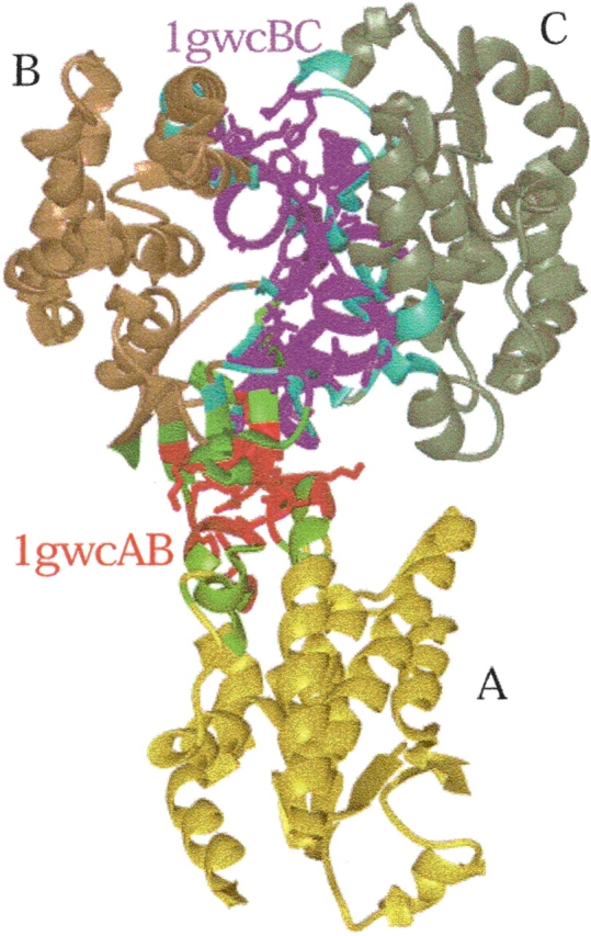
Definition of protein–protein interfaces: The ribbon diagram of Glutathione S-Transferase is displayed. The three chains (A, B, and C) of transferase are colored yellow, gold, and dark green, respectively. Two interfaces form between chain pairs. Chains A and C do not form an interface. In the first interface between chains A and B, the interacting residues are colored red, and the nearby ones in green. In the second one (interface between chains B and C), the interacting residues are displayed in magenta and the nearby in cyan. Only the side chains of the interacting residues are shown.

We have applied these criteria to all multichain PDB entries in the database. On July 18, 2002, there were 18,687 entries in the PDB that included 35,112 single chains. PDB entries that contain more than two chains were used to get two-chain combinations. Therefore, interfaces between any two chains were extracted if each of the two chains at least had 10 residues. These included all two-chain interfaces from dimers, trimers, and higher complexes of protein–protein and protein–peptide complexes. As a result, 21,686 two-chain interfaces were obtained. Following the nomenclature of Tsai et al. (1996), we have renamed the interfaces as follows: If the PDB code of a protein is 1gwc and it has two chains A and B, the interface is named 1gwcAB (see Fig. 1 ▶), indicating that there is an interface between chains A and B of protein 1gwc.

Structural comparisons

Constructing a data set of nonredundant interfaces is not straightforward. The main difficulty is that interfaces consist of two separate chains with discontinuous pieces of the polypeptides. Although we seek similar spatial arrangements of the polypeptide pieces between the interfaces, their sequence order may differ. Furthermore, some of the pieces may consist of isolated amino acids. Consequently, any algorithm that is sequence- and directionality-dependent is not applicable to the interface comparison problem. On the other hand, computer vision-based structural alignment techniques view protein structures as collections of points in 3D space. Therefore, they are ideally suited to comparisons between protein surfaces and interfaces (Nussinov and Wolfson 1991; Tsai et al. 1996). The algorithms used in this study compare all available protein interfaces, allowing the clustering of the interfaces into families with distinct structural features.

The first step is the comparison of interfaces by the Geometric Hashing algorithm. Details of the algorithm were given in Tsai et al. (1996) and in Nussinov and Wolfson (1991). The algorithm uses the C^α coordinates and no connectivity among these C^α points is taken into account in the matching. Figure 2a ▶ shows a protein in 3D space representation with its C^α atoms denoted as points. This is the same protein as in Figure 1 ▶ (the same view). The goal of the algorithm is to find the most similar sets of points common to both protein interfaces. The algorithm has three consecutive steps: hash table construction, voting, and extension processes.

Figure 2.

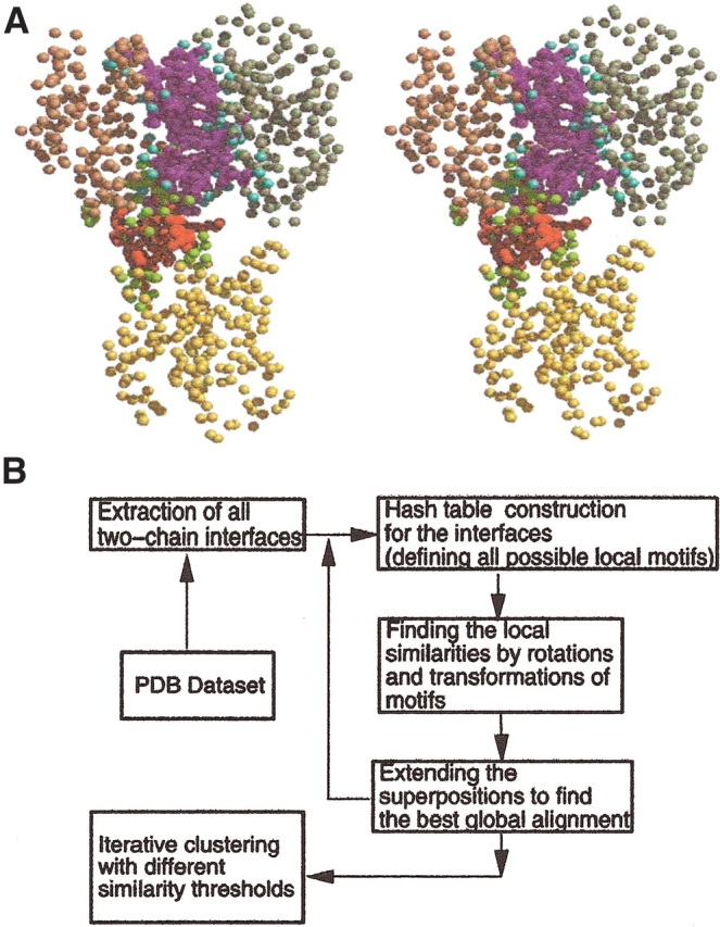
(A) The input of the alignment program for interfaces: the representation of the Glutathione S-Transferase with its C^α atoms as points in three-dimensional space. The coloring scheme is as in Figure 1 ▶. The structural pairwise alignment of interfaces are performed considering only the points belonging to the contacting and nearby atom. (B) The schematic representation of the alignment algorithm. We start with all structures available in the PDB and extract the interfaces formed between pairs of chains. These interfaces are next compared to each other with an iterative procedure to assign them into different structural clusters. The algorithm reads the interfaces as sets of points—as shown in A—and constructs the hash tables to define all local motifs in interfaces. Interfaces are compared iteratively and clustered.

1. Hash table construction is used to find the local similarity between two sets of points. The coordinates of every three consecutive C^α (C_i−1, C_i, C_i+1) along the protein chain define an orthogonal reference frame, centering the (C_i) point as follows: Rx = C_i−1 − C_i; V_t = C_i+1 − C_i; R_z = R_x x V_t; R_y = R_x x R_z; where R_x, R_y, R_z are the x, y, z axes of the reference frame and x represents the cross-product. Each point within a cutoff distance of 15 Å around the i′th point is projected onto this orthogonal reference frame. Thus, for the i′th element in the table, both the identity of the C^α atom and the neighboring projected coordinates are kept. This is the preprocessing step.

2. Voting is carried out to compare the two structures. If a local similarity (a large “enough” number of votes for a given reference frame) is detected between the two proteins, the transformation is computed and the matching C^α atom pairs from the two proteins are superimposed. The similarity between the proteins is computed in terms of the root mean squared deviation (RMSD) between them.

3. The extension step is used to find the best global alignment starting with the best local alignment obtained in the previous step. This is an iterative process. The interfaces are superimposed, and a new list of matching pairs is reassigned, with the distance between every matched pair below a threshold (here 2.5 Å). If the distance criterion cannot find a unique solution, the best global alignment is found using the similarity score. This score favors solutions with better connectivity. For complete description of the method see Tsai et al. (1996), Nussinov and Wolfson (1991), Bachar et al. (1993), and Fischer et al. (1994).

In this study, the measure of the similarity between two protein–protein interfaces is based on the extent of the geometrical superposition between their corresponding C^α atoms, the percent residue identity in the match, and the difference in sizes between the interfaces. The superposition between two interfaces computed by the Geometric Hashing algorithm yields a list of matched C^α atom pairs. The percent residue identity is the count of identical residues in the match divided by the total number of matched pairs. The RMSD is not considered in measuring the similarity between two interfaces. Instead, we compute a “connectivity score” to express the quality of a geometrical superposition. If the residue connectivity information is excluded, the similarity score is equal to the number of matched pairs. The data set contains both biological (functional) and crystal packing interfaces, because unfortunately, to date, there is no clear way to distinguish between them. Nevertheless, because crystal interfaces are often small, we exclude an interface if it has less than 10 residues that are in contact in a given chain.

The clustering algorithm

Clustering is a multivariate problem with two criteria. First, members in each cluster should be similar to each other, and second, members of one cluster should be different from members of all others (Gordon 1981). The frequently adopted clustering approach for classifying a set of structures consists of two steps. First, the similarity between any two structures is calculated, and second, a set of clusters is generated by clustering the two most similar structures at a time and selecting one of them to represent the cluster. This procedure is iterated, until the extent of similarity between the unclustered structures and the cluster representative is below the specified threshold. Here, we have adopted a heuristic iterative clustering procedure. At each iteration cycle, the similarity definition is gradually relaxed. This yields a hierarchy of grouping of clusters with different similarity thresholds. In the first phase of an iteration, the first entry in the initial list of interfaces forms a new cluster. The next interface in the list is compared to the first. If the similarity between them is above a predefined threshold, the second is added to the cluster of the first, or else it forms a new cluster. Next, the third interface is compared with the clusters already formed. This procedure is repeated, until all structures are assigned to clusters. At the end of this procedure, the similarity between each member of the individual cluster and its corresponding putative representative should be above the threshold prescribed for the current clustering cycle. In this phase, pairwise structural comparisons of structures are carried out sparsely, greatly reducing the computational costs. In the second phase, exhaustive pairwise comparisons are performed within each cluster. These extensive comparisons fulfill two functions. First, the structure that is most similar to all other structures in its cluster is selected as the representative for the next iteration. Second, if a structure is found dissimilar to other structures, it is removed from the cluster. Such a structure forms a new, one-member cluster for the next iteration. A schematic representation of the algorithm is given in Figure 2B ▶. This clustering procedure is as that used previously (Tsai et al. 1996).

Discussion

The data set at the different clustering cycles

Table 1 lists the threshold parameters applied in successive clustering cycles to calculate the similarities between interfaces. The first column gives the iteration cycle. There are six successive clustering cycles (A through F). The second column gives the number of interface clusters at the beginning and end of the iteration. For example, during iteration A, there were initially 21,686 interfaces (in the first cycle, this number is equal to the number of two-chain interfaces in the PDB). Using the similarities of the structures and sequences (with the parameters listed in columns 3–5) the number decreased to 16,446. The connectivity score takes into account the residue connectivity in the polypeptide chains. The score favors a match with consecutive residues. At the end of the sixth (final) cycle, we obtained 3799 distinct clusters. After this cycle, members of each cluster had at least 0.5 connectivity score. There was no amino acid similarity constraint and the maximal size difference between interfaces was 50 residues.

Table 1.

The parameters used during the clustering of the interfaces

Cycle	Number of interfaces	Relative connectivity score	Minimal % amino acid identity	Maximal amino acid size difference between interfaces
A	21,686 → 16,446	0.9	90	0
B	16,446 → 9637	0.9	80	3
C	9637 → 6647	0.8	50	10
D	6647 → 5332	0.7	25	20
E	5332 → 4429	0.6	10	40
F	4429 → 3799	0.5	0	50

A comparison of the new and old data sets of interfaces shows a substantial increase, from 351 to 3799. The data set and the clustering results are available at http://protein3d.ncifcrf.gov/~keskino/ and http://home.ku.edu.tr/~okeskin/INTERFACE/INTERFACES.html. It is of interest to examine whether this increase is the outcome of the increased number of PDB entries or of new architectures. Figure 3 ▶ shows the ratio of increase in the PDB entries, the SCOP families (the 1996 and 2002 versions, respectively; Murzin et al. 1995) and in the interface clusters (the old data set [Tsai et al. 1996] and this work). We observed that the number of entries in the PDB increased sixfold and the number of SCOP families increased threefold, whereas the increase of interface clusters is 10-fold. Thus, it appears that the increase in the PDB over the last seven years has allowed a more diversified data set for interfaces. This may also be the outcome of the rapid growth in the determination of high molecular weight proteins that are likely to include more than one chain.

Figure 3.

Histogram indicating the increase in the number of protein structures available in the PDB (between 1997 and 2003), the increase in the number of protein–protein interface clusters (comparison between the previous work [Tsai et al. 1996] and the results of this work), the increase in the number of protein families (comparison between the 1997 and 2003 SCOP databases). Note that our previous interface data set was extracted in 1996, so the closest version of the SCOP (1997) was compared in the analysis.

Generation of a nonhomologous data set of interfaces: Sequence alignment, excluding chains with high sequence similarity

To have a nonredundant set of interfaces, sequences within each family were compared using CLUSTALW (Higgins et al. 1994) and the BLOSSUM90 substitution matrix (Henikoff and Henikoff 1992). To eliminate redundancy, a threshold similarity of 50% was imposed. Thus, one of the two sequences in a cluster that shares a sequence similarity of more than 50% is deleted from the cluster. This yields a data set of interfaces with structurally similar but sequentially dissimilar members. Further, to constitute a valid cluster of interfaces, the cluster should have at least five members (10 chains). These filtering procedures reduce the number of clusters from 3799 to 103.

The 3799 original clusters listed by their representatives are given in Appendix A (and are available at our Web site at http://protein3d.ncifcrf.gov/~keskino/). The numbers in parentheses are the number of all members included in the corresponding clusters. In all cases, both chains of the interface of each cluster member superimpose on those of the cluster representative within the similarity criteria provided in Table 1. Appendix B lists the nonredundant interface clusters. These clusters have at least five members, and at most 50% sequence identity among their members. This separate listing is given for the convenience of users who wish to carry out statistical analysis of the data set. We have further carried out multiple structure comparisons of all cluster members listed in Appendix B, using MultiProt (Shatsky et al. 2002, 2003). Appendices A and B are provided as Supplemental Material. Clusters for which MultiProt detected a consensus core encompassing all members from both chains and with similar function were labeled as Type I, those with different functions were labeled as Type II. On the other hand, the clusters where MultiProt found a consensus for only one of the chains, were termed Type III. Fifty-four of the clusters are Type I and II interfaces; the rest are Type III aligned interfaces.

Multiple structural alignment of the interfaces with MultiProt

MultiProt detects recurring motifs in an ensemble of proteins by simultaneously aligning multiple protein structures (Shatsky et al. 2002, 2003). The algorithm considers all protein structures at the same time, rather than initiating from a pairwise-imposed molecular seed. This eliminates the bias in the superposition and finds the largest common substructure of C^α atoms that appears in the structural set. Furthermore, MultiProt efficiently finds high-scoring partial multiple alignment for all possible number of molecules in the input. That is, it does not require that all input molecules participate in the alignment. Because it is sequence order-independent, it can be applied to protein surfaces and protein–protein interfaces effectively. We have used MultiProt to align the interfaces of our clusters to find consensus motifs of the members’ interfaces. To qualify as a consensus motif, at least 10 residues have to match with an RMSD of at most 3.5 Å. Because each member can have noncontiguous residues in the interface, MultiProt is an extremely useful tool for our purpose.

Interface family types

Type I: Similar interfaces, similar global protein folds

In most cases, if the interfaces are similar, the overall protein folds are also similar. Such similar interface, similar fold clusters contain a single family. The list of the interface clusters and the members of these clusters are given in Appendix B (nonitalic entries). The interface clusters include homodimeric enzyme complexes (transferases, oxidoreductases, etc.), enzyme/inhibitor complexes, antibody/antigen complexes, as well as toxins. They have different polar/nonpolar compositions and different accessible surface areas. Some examples are given in Figure 4 ▶. In the figure three members of the 1cydAD cluster are presented. This cluster is formed by reductases, oxidoreductases (PDB codes: 1cyd, 1e3s, 1hdc, 1i01), and a pterin reductase (PDB code: 1e92).

Figure 4.

Some examples of similar interfaces, similar monomer structures, and functions (called Type I in this work). In the figure three members of the 1cydAD cluster are presented. The two complexes displayed at the top panel are oxidoreductases (PDB codes: 1cyd, 1e3s), and the bottom complex is a pterin reductase (PDB code: 1e92). Three of the structures are available as tetramers in the PDB. For clarity, we have displayed the chains that form the common interface among them (1cydAD, 1e3sAC, and 1e92AC). In all complexes one chain is colored pink, and the other is cyan. One side of the common interfaces is colored yellow, and the complementary side of the interfaces is colored in purple. There are 111 interface residues in common. The RMSD between the 1cydAD and 1e3sAC interfaces is 3.11 Å, and the rmsd between 1e92AC and 1e3sAC interfaces is 1.26 Å.

Type II: Similar interfaces, dissimilar global protein folds

Some clusters, belong to a particularly interesting category: In these cases the interfaces are structurally similar; however, the global protein folds are different. These are listed in Table 2 and Appendix B (italic entries). These similar-interfaces, dissimilar-protein folds fall into different families (see the SCOP classification, also provided in Table 2, first column). Even though, however, they have structurally similar interfaces, they are nevertheless members of the same clusters. These families have different functions. Thus, interface structural similarity does not ensure global protein structural similarity. Furthermore, previously it has been shown that globally similar structures may have different functions in proteins (Martin et al. 1998; Orengo et al. 1999; Moult and Melamud 2000; Thornton et al. 2000; Nagano et al. 2002). Cases such as those listed here illustrate that this paradigm can be taken further: Similar interfaces do not imply similar functions.

Table 2.

Similar interfaces with dissimilar folds

SCOP family	Representative	Proteins	Common residues in interfaces	Interface fold type
[1] DNA polymerase processivity factor	1ah8AB	[1] GP45 sliding clamp (1b77AB) [1] Prolifirating cell nuclear antigen (PCNA) (1axcAC)	18	α + β
[2] Microbial ribonucleases		[2] Barnase/Binase (1a2pBC)
[1] Chromo domain-like chromatin	1afrBD	[1] Heterochromatin protein 1, HP1 (ldz1AB, 1e0bAB)	22	α
[2] Aldolase		[2] Transaldolase (1f05AB)
[3] Tryptophan synthase β subunit-like PLP-dependent enzymes		[3] 1-aminocyclopropane-1-carboxylate deaminase (1f2dBD)
[1] Cellulose-binding domain family III	1aohAb	[1] Cohesin domain (1aohAB, 1g1kAB)	21	β
[2] Fluorescent proteins		[2] Green fluorescent protein (1b9cAB) [2] Red fluorescent protein (1g7kAB)
[1] Snake venom toxins &	1e7kAB	[1] Cardiotoxin V4II (1cdtAB)	19	β
[2] Cysteine proteinases		[2] (Pro)cathepsin X(1ef7AB)
[3] P-loop containing nucleotide triphosphate hydrolases		[3] Initiation factor 4a (1fuuAB)
[1] MHC antigen-recognition domain	1hyrAC	[1] Bungarotoxin (1kbaAB) [1] MHC I homolog (1hyrAC, 1kcgac)	20	—
[2] Tyrosine-dependent oxidoreductases		[2] Negative transcriptional regulator NmrA (1k6jAB)
		[3] Class I MHC-related molecule (1kcgAC)
[1] Virus ectodomain	1qbzBC	[1] Core structure of Ebo gp2 (1eboAB)	54	α (bundle)
[2] Tropomyosin		[2] Tropomyosin (1ic2CD)
		[1] Envelope polyprotein GP160 (1if3AB) [1] Retrovius gp41 protease-resistant core (1qbzAC)
[1] Fibrinogen C-terminal domain-like	1gk4AB	[1] Fibrinogen C-terminal domains (1fzaAB)	73	α (bundle)
[2] Vimentin coil		[2] Vimentin coil (1gk4AB)
[3] Neuronal synaptic fusion complex		[3] Neuronal synaptic fusion complex (1gl2BC, 1kilAB)
[4] Tropomyosin		[4] Tropomyosin (1ic2AB)
[5] Synaptic snare complex		[5] Synaptic vesicle protein vamp2 and presynaptic plasma membrane proteins snap-25 and syntaxin 1a (2bu0BC)
[1] Immunoglobulin	1irxAB	[1] T-cell antigen receptor (1fo0HB, 1g6rBH)	13	α
[2] Ferritin		[2] (Apo)ferritin (1iesBF)
[3] Nucleotidylyl transferase		[3] C-terminal domain of class I lysyl-tRNA synthetase (1irxAB)
[1] Tetraspanin	1g8qAB	[1] CD81 extracellular domain (1g8qAB)	20	α
[2] Signaling proteins		[2] Dopamine D2 receptor modeled on bacteriorhodopsin (1i15cd)
[3] Light-harveting complex subunits		[3] Light-harvesting complex subunits (1ijdac, 1lghgj)
[1] α helical bundle	1gc7AB	[1] α helical bundle (1cosAC)	31	α
[2] Neuronal synaptic fusion complex		[2] Neuronal synaptic fusion complex (1gl2AC, 1kilAC, 1kilBD)
[3] Virus ectodomain 2siv		[3] Retrovius gp41 protease-resistance core (2sivAB)
[1] ROP protein	1kd8AB	[1] ROP protein (1f4mAB)	43	α
[2] Neuronal synaptic fusion complex		[2] Neuronal synaptic fusion complex (1hvvBC)
[3] Leucine zipper-domain		[3] GCN4 (1kd8AB)
[4] Tropomyosin		[4] Tropomyosin (1kqlAB)
[5] Cell envelope component		[5] Murein lipoprotein (1mlpAB)
[1] Virus ectodomain	2sivAC	[1] Retrovius gp41 protease-resistant core (1aikNC)	29	α
[2] Cytochrome c		[2] Mitochondrial cytochrome c (1kyoBR)
[3] Neuronal synaptic fusion complex		[3] Neuronal synaptic fusion complex (1sfcBD, 1sfcBJ)
[1] Bcr-Abl oncoprotein oligomerization domain homotetramer	1l7cAC	[1] Bcr-Abl oncoprotein oligomerization domain (1k1fDF)	17	α
[2] Membrane protein		[2] Pentameric transmembrane domain of phospholamban (1k9nAB)
[3] α-catenin/vinculin		[3] α-catenin (1l7cAC)
[4] Nucleotide and nucleoside kinases		[4] Thymidylate kinase (3tmkDG)

The first column is the SCOP classification. The numbers in square brackets identify the different SCOP families within each cluster. The second column lists the representatives of the interface clusters. The third column provides the individual members in the corresponding cluster. The interface names are represented by their PDB codes and chain identifiers. The numbers at the beginning of the proteins represent which SCOP family—in column 1—it belongs to. The fourth column is the result of MultiProt (Shatsky et al. 2002, 2003) alignments: the number of common residues aligned structurally for the members in the clusters. The fifth column gives the interface fold type.

Figure 5 ▶ illustrates some examples from Table 2. Part A shows all members of the cluster. Each case in the figure presents the ribbon diagrams of the proteins that belong to different SCOP families in the same interface cluster, clearly showing that the global structures are different. Part B displays ribbon diagrams of two of the proteins with their common interfaces highlighted with yellow. Note that there are three clusters in Table 2 where the representative of the cluster does not appear in the list of family members. These cases are cellulose-binding domain family III, MHC antigen-recognition domain, and nucleotide and nucleoside kinases. In these cases, while the representative aligned with each cluster member, it did not align well with all members simultaneously, suggesting some slight deviations in the multiple structural superposition.

Figure 5.

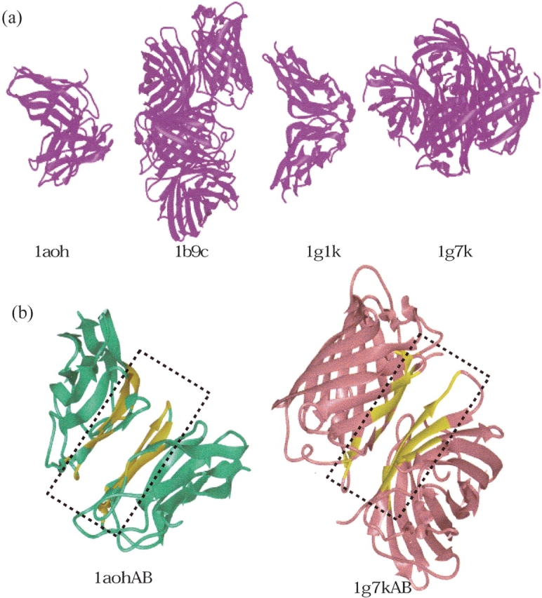
Some examples of similar interfaces, dissimilar monomer structures, and functions (called Type II in this work). (A) In the figure, ribbon diagrams of four members in the 1g1kAB cluster are illustrated. These are the structures of the single cohesin domain from the scaffolding protein cipa of the Clostridium thermocellum cellulosome (1aoh), green fluorescent protein mutant F99S, M153T, and V163A (1b9c), cohesin module from the cellulosome of Clostridium cellulolyticum (1g1k), and Dsred, a red fluorescent protein from discosoma sp. red (1g7k). The letters correspond to the monomers in these complexes. (B) Ribbon diagrams of two interfaces (1aohAB and 1g7kAB) derived from two functionally different proteins. The yellow region points to the common interface with 48 common interface residues. The rmsd between these two interfaces is 2.31 Å, considering only α-carbon atoms.

Type III: One side similar interfaces, dissimilar global protein folds

Our data set also contains clusters where one chain of the interface is conserved while the second varies. Figure 6 ▶ presents an example of such a cluster. Although this figure specifically shows an antibody interacting with four partners (three of them peptides), Type III interfaces are not constrained to only antibody/antigen or protein/peptide complexes. This type manifests protein complexes with a diverse range of biological functions. For example, in one of the Type III clusters we have a homodimer antioncogene protein (interface ID: 1a1uAC), a homodimer of leucine zipper complex (interface ID: 1a93AB), a homodimeric complex of mannose binding protein, lectin (interface ID: 1afa12), a homodimer of transcription regulation protein (interface ID: 1ajyAB), a tetramer of cytokine, cliary neurotrophic factor protein (1cnt14), and a homodimeric replication termination protein (1f4kAB). One-chain conserved clusters are very interesting: They can be used to address fundamental questions such as whether nonspecific binding is largely hydrophobic with flatter surface, which functions are involved, or whether in one chain-dominant interfaces the second chain is smaller. The data set may bear on longstanding problems relating to binding specificity and selectivity and to specificity with respect to conserved interactions and function. It may also be useful for prediction of residues contributing dominantly to stability.

Figure 6.

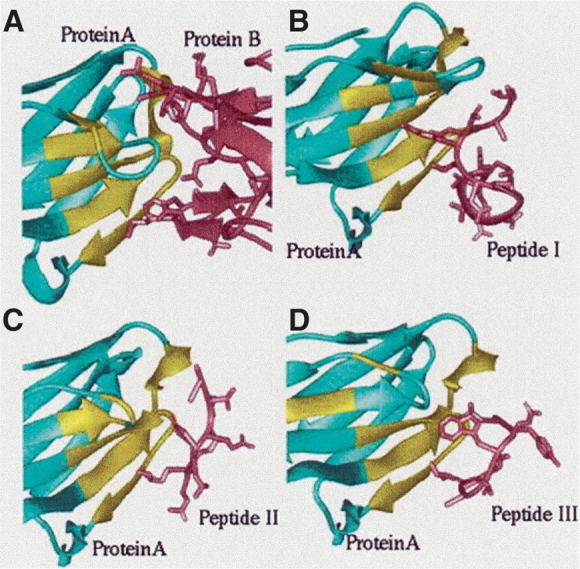
The ribbon diagrams of Type III interfaces. The members in this cluster are represented by the 1fj1DE interface. In all figures, the cyan structures represent the protein that binds to different proteins or peptides (pink structures). The yellow colored region in each case is the similar interface architecture within the 1fj1DE cluster. (A) This displays an example of a complex between a human monoclonal BO2C11 FAB heavy chain and human factor VII (1iqdBC interface). (B) An illustration of an antibody/peptide complex (1bogBC interface). (C) This is another immunoglobulin/viral peptide complex formed between the FAB fragment and human rhinovirus capsid protein VP2 (1a3rHP interface). (D) This is an example for the interface formed between the heavy chain (IGG2A Kappa antibody CB41) and an antigen bound peptide (1cfsBC interface). The RMSD values between the interfaces are 0.67 Å, 1.29 Å, and 3.01 Å over 26 residues, respectively.

Propensities of residues in the interfaces

The relative frequencies of different types of amino acids in the interfaces of protein–protein complexes can be used to derive the propensities of the residues. The overall propensities of the 20 amino acids are calculated for the contacting residues (not including the “nearby”) in the interfaces from the data set containing all interface clusters. We compare the frequency patterns at the binding sites versus those in the overall structures. The propensity (P_i) of a residue (i = Ala,Val, Gly, . . .) to occur at the interface is calculated as the fraction of the count of residue i in the interface compared with its fraction in the whole chain as

(1)

where n_i is the number of residues of type i at the interface, N_i is the number of residues of type i in the chains, n is the total number of residues in the interface, and N is the total number of residues in the whole chains.

Figure 7 ▶ displays the correlation of our residue propensities with those of Jones and Thornton (1997). The axes represent the natural logarithms of the propensities. The positive value in the logarithmic propensity indicates that a residue is more likely to occur in an interface. A high correlation coefficient (0.91) is obtained over the 20 amino acids. The residue propensities of Jones and Thornton (1997) were calculated from a data set of 63 protein complexes by taking the fraction of accessible surface area that the amino acid has contributed to the interface compared with the fraction of accessible surface area that the amino acid has contributed to the whole surface (i.e., all exposed residues). Thus, their propensities are calculated by the propensity of the accessible surface areas of the residues. Our propensities are calculated by the frequency of occurrence of the residues compared with the rest of the chain. To have a more appropriate comparison, we have multiplied each residue by its average accessible surface area (Miller et al. 1987) and normalized the results by the surface propensities of the amino acids (Table 2; Ma et al. 2003) according to the formula: ln(P)_i = ln[(n_i/N_i)/(n/N)/(n_s/Ns)/(n/N) * ASA], where ASA stands for the average accessible surface areas of the residues in an extended Gly-X-Gly triplet (Miller et al. 1987). The high correlation we observe suggests that their data set, despite its smaller size, still presents a good coverage with similar properties.

Figure 7.

Propensities of residues in the interfaces. This figure illustrates the correlation of our residue propensities with those of Jones and Thornton 1997. The axes represent the natural logarithms of the propensities. A high correlation coefficient (0.91) is obtained over the 20 amino acids.

Table 3 lists the propensities of the different amino acids in interfaces Type I, Type II, and Type III. We have further computed the propensities in each interface type when dividing the residues into classes of hydrophobic (A,P,L,I,M,V), charged (D,E,R,K), polar (N,Q,S,T), and aromatic residues (W,Y,F,H). The last four rows of Table 3 give the overall contribution of these residue classes. The percentages are given as the second figure in the last four rows. Clearly, interfaces are dominated by hydrophobic residues in all three cases. Next, it is mostly aromatic residue contribution. However, it is interesting that the hydrophobic effect is smaller in the Type III interfaces. Instead, the propensities of the charged residues increase. This may reflect the fact that in Type III the nonconserved side of the interface is smaller. Smaller interfaces have already been shown to display a reduced hydrophobic effect (Tsai et al. 1997). In these smaller, more exposed interfaces electrostatics appears to play a more important role. In general, overall, charged residues are less frequent in the interfaces. This also suggests that overall electrostatic interactions are probably not the major source of the stability of the interfaces.

Table 3.

Residue propensities of amino acids

Residue type	Type I	Type II	Type III	All
G	0.699	0.599	0.644	0.671
A	0.966	0.761	0.897	0.900
C	1.780	1.338	1.153	1.427
D	0.966	0.602	0.775	0.826
E	0.725	0.988	0.982	0.866
F	1.409	1.373	0.956	1.213
H	1.331	0.779	0.900	1.076
I	1.044	1.469	0.999	1.068
K	0.611	0.578	0.887	0.732
L	1.073	1.532	1.039	1.127
M	1.289	0.839	0.982	1.083
N	0.908	1.215	1.261	1.109
P	0.987	0.343	0.626	0.735
Q	0.910	1.1014	0.951	0.954
R	1.137	0.754	1.276	1.140
S	1.027	1.029	0.864	0.955
T	0.878	0.741	1.080	0.942
V	0.999	1.112	0.865	0.986
W	0.969	0.856	1.260	1.075
Y	1.560	1.379	1.102	1.318
A,P,I,L,M,V	7.50–38%	7.42–40%	6.36–34%
D,E,R,K	3.45–17%	2.92–16%	3.93–21%
N,Q,S,T	3.73–19%	3.98–20%	4.15–22%
W,Y,F,H	5.27–26%	4.40–24%	4.22–23%

The first column is the type of the amino acid. The second, third, and fourth columns are the propensities for Type I, II, and III clusters, respectively. The last column gives the overall propensities summed over all types of interfaces. The last four rows are the sum of the propensities for hydrophobic, polar, charged, and aromatic residues, respectively. The first number gives the cumulative effect of all the residues in the four classes, the second number gives the percentage of the each class.

Conclusions

Here we provide a structurally unique data set of two-chain interfaces derived from the PDB. The interfaces are clustered based on their spatial structural similarities, regardless of the connectivity of their residues on the protein chains. The data set includes 3799 clusters, compared to 351 in 1996. This substantially more diverse data set reflects both the growth in the number of structures as well as the larger number of higher molecular weight proteins currently in the PDB. The comparison of the old and new data sets indicates that the number of newly found interface clusters has increased much more rapidly compared to the number of the available new PDB structures. This may suggest that the number of unique interfaces has still not reached its upper limit.

We divide the clusters into three types: Type I clusters consist of similar interfaces whose parent chains are also similar. In Type II clusters, the interfaces are similar; however, the overall structures of the parent proteins from which the interfaces derive are different. In all Type II cases that we have studied, the clustered proteins belong to different SCOP families, with different functions. Type III category introduces clusters of interfaces where only one side of the interface is similar but the other side differs. Type III clusters illustrate that a binding site can interact with more than one chain, with different geometries, sizes, and composition. One of the paradigms in protein science states that similar global structures may have similar functions. Our observations suggest an extension of this paradigm: Similar interface architectures may have differerent functions. As in protein structures, evolution has reused “good” favorable interface structural scaffolds and adapted them to diverse functions. The functions extend from enzymes/inhibitors to toxins and immunoglobulins. We did not observe homodimers in Type II clusters. This is probably due to the smaller sizes of the monomers and the extensive interfaces in the two-state homodimers that cover large portions of the chains. As expected, we find that multifunctional interface clusters consisting of helices largely derive from proteins whose functions relate to muscle and to membranes.

The observation that globally different protein structures associate in similar ways (i.e. Type II) to yield similar motifs, is interesting. Clearly, there is a very large number of ways that monomers can combinatorially assemble. Remarkably, among these there are preferred interface architectures, and these are similar to those observed in monomers (Tsai et al. 1998b). This observation both underscores the view that the number of favorable motifs is limited in nature, and highlights the analogy between binding and folding. It is further reminiscent of the combinatorial assembly of protein building blocks in folding (Tsai and Nussinov 1997).

We hope that this diverse, structurally nonredundant data set will be useful in a broad range of studies, such as deriving profiles of binding sites, elucidation of the determinants of protein–protein interactions, and identification of residues contributing to the stabilization of the protein associations and those playing a role in a specific protein function. The data set should allow extensive comparisons between binding and folding and derivation of motifs across interfaces. This data set should further be useful in construction of protein networks, and allow studies of structurally conserved residue hot spots. We expect it to be useful in studies of evolutionary conservation, recognition, binding, and function.

Electronic supplemental material

Supplemental material includes two appendices: (1) a list of 3,799 cluster representatives; (2) a list of all nonredundant two-chain interface clusters.

References

- Arkin, M.R., Randal, M., DeLano, W.L., Hyde, J., Luong, T.N., Oslob, J.D., Raphael, D.R., Taylor, L., Wang, J., McDowell, R.S., et al. 2003. Binding of small molecules to an adaptive protein–protein interface. Proc. Natl. Acad. Sci. 100 1603–1608. [DOI] [PMC free article] [PubMed] [Google Scholar]
- Bachar, O., Fischer, D., Nussinov, R., and Wolfson, H. 1993. A computer vision based technique for 3-D sequence-independent structural comparison of proteins. Protein Eng. 6 279–288. [DOI] [PubMed] [Google Scholar]
- Berman, H.M., Westbrook, J., Feng, Z., Gilliland, G., Bhat, T.N., Weissig, H., Shindyalov, I.N., and Bourne, P.E. 2000. The Protein Data Bank. Nucleic Acids Res. 28 235–242. [DOI] [PMC free article] [PubMed] [Google Scholar]
- Bogan, A.A. and Thorn, K.S. 1998. Anatomy of hot spots in protein interfaces. J. Mol. Biol. 280 1–9. [DOI] [PubMed] [Google Scholar]
- Brooijmans, N., Sharp, K.A., and Kuntz, I.D. 2002. Stability of macromolecular complexes. Proteins 48 645–653. [DOI] [PubMed] [Google Scholar]
- Chakrabarti, P. and Janin, J. 2002. Dissecting protein–protein recognition sites. Proteins 47 334–343. [DOI] [PubMed] [Google Scholar]
- Chothia, C. 1992. Proteins. One thousand families for the molecular biologist. Nature 357 543–544. [DOI] [PubMed] [Google Scholar]
- Chothia, C. and Janin, J. 1975. Principles of protein–protein recognition. Nature 256 705–708. [DOI] [PubMed] [Google Scholar]
- Cunningham, B.C. and Wells, J.A. 1991. Rational design of receptor-specific variants of human growth hormone. Proc. Natl. Acad. Sci. 88 3407–3411. [DOI] [PMC free article] [PubMed] [Google Scholar]
- DeLano, W.L. 2002. Unraveling hot spots in binding interfaces: Progress and challenges. Curr. Opin. Struct. Biol. 12 14–20. [DOI] [PubMed] [Google Scholar]
- DeLano, W.L., Ultsch, M.H., deVos, A.M., and Wells, J.A. 2000. Convergent solution to binding at a protein–protein interface. Science 287 1279–1283. [DOI] [PubMed] [Google Scholar]
- Fariselli, P., Pazos, F., Valencia, A., and Casadio, R. 2002. Prediction of protein–protein sites in heterocomplexes with neural networks. Eur. J. Biochem. 269 1356–1361. [DOI] [PubMed] [Google Scholar]
- Fernández, A. and Scheraga, H.A. 2003. Insufficiently dehydrated hydrogen bonds as determinants of protein interactions. Proc. Natl. Acad. Sci. 100 113–118. [DOI] [PMC free article] [PubMed] [Google Scholar]
- Fischer, D., Wolfson, H., Lin, S.L., and Nussinov, R. 1994. Three-dimensional, sequence order-independent structural comparison of a serine protease against the crystallographic database reveals active site similarities: Potential implications to evolution and to protein folding. Protein Sci. 3 769–778. [DOI] [PMC free article] [PubMed] [Google Scholar]
- Gordon, A.E. 1981. Classification: Methods for the exploratory analysis of multivariate data. Chapman and Hall, New York.
- Henikoff, S. and Henikoff, J. 1992. Amino acid substitution matrices from protein blocks. Proc. Natl. Acad. Sci. 89 10915–10919. [DOI] [PMC free article] [PubMed] [Google Scholar]
- Hu, Z., Ma, B., Wolfson, H., and Nussinov, R. 2000. Conservation of polar residues as hot spots at protein interfaces. Proteins 39 331–342. [PubMed] [Google Scholar]
- Jones, S. and Thornton, J.M. 1996. Principles of protein–protein interactions. Proc. Natl. Acad. Sci. 93 13–20. [DOI] [PMC free article] [PubMed] [Google Scholar]
- ———. 1997. Analysis of protein–protein interaction sites using surface patches. J. Mol. Biol. 272 121–132. [DOI] [PubMed] [Google Scholar]
- Katchalski-Katzir, E., Shariv, I., Eisenstein, M., Friesem, A.A., Aflalo, C., and Vakser, I.A. 1992. Molecular surface recognition: Determination of geometric fit between proteins and their ligands by correlation techniques. Proc. Natl. Acad. Sci. 89 2195–2199. [DOI] [PMC free article] [PubMed] [Google Scholar]
- Keskin, O., Bahar, I., Badretdinov, A.Y., Ptitsyn, O.B., and Jernigan, R.L. 1998. Empirical solvent-mediated potentials hold for both intra-molecular and inter-molecular inter-residue interactions. Protein Sci. 7 2578–2586. [DOI] [PMC free article] [PubMed] [Google Scholar]
- Kleanthous, C. 2000. Protein–protein recognition. In Frontiers in molecular biology (ed. C. Kleanthous). Oxford University Press, New York.
- Kuhlmann, U.C., Pommer, A.J., Moore, G.R., James, R., and Kleanthous, C. 2000. Specificity in protein–protein interactions: The structural basis for dual recognition in endonuclease colicin–immunity protein complexes. J. Mol. Biol. 301 1163–1178. [DOI] [PubMed] [Google Scholar]
- Kumar, S. and Nussinov, R. 2001. Fluctuations in ion pairs and their stabilities in proteins. Proteins 41 485–497. [DOI] [PubMed] [Google Scholar]
- Kuntz, I.D., Chen, K., Sharp, K.A., and Kollman, P.A. 1999. The maximal affinity of ligands. Proc. Natl. Acad. Sci. 96 9997–10002. [DOI] [PMC free article] [PubMed] [Google Scholar]
- Lichtarge, O., Bourne, H.R., and Cohen, F.E. 1996. An evolutionary trace method defines binding surfaces common to protein families. J. Mol. Biol. 257 342–358. [DOI] [PubMed] [Google Scholar]
- LoConte, L., Chothia, C., and Janin, J. 1999. The atomic structure of protein–protein recognition sites. J. Mol. Biol. 285 2177–2198. [DOI] [PubMed] [Google Scholar]
- Ma, B., Wolfson, H.J., and Nussinov, R. 2001. Protein functional epitopes: Hot spots, dynamics and combinatorial libraries. Curr. Opin. Struct. Biol. 11 364–369. [DOI] [PubMed] [Google Scholar]
- Ma, B., Shatsky, M., Wolfson, H.J., and Nussinov, R. 2002. Multiple diverse ligands binding at a single protein site: A matter of pre-existing populations. Protein Sci. 11 184–197. [DOI] [PMC free article] [PubMed] [Google Scholar]
- Ma, B., Elkayam, T., Wolfson, H., and Nussinov, R. 2003. Protein–protein interactions: Structurally conserved residues distinguish between binding sites and exposed protein surfaces. Proc. Natl. Acad. Sci. 100 5772–5777. [DOI] [PMC free article] [PubMed] [Google Scholar]
- Martin, A.C.R., Orengo, C.A., Hutchinson, E.G., Jones, S., Karmirantzou, M., Laskowski, R.A., Mitchell, J.B.O., Taroni, C., and Thornton, J.M. 1998. Protein folds and functions. Structure 6 875–884. [DOI] [PubMed] [Google Scholar]
- Miller, S., Janin, J., Lesk, A.M., and Chothia, C. 1987. Interior and surface of monomeric proteins. J. Mol. Biol. 196 641–656. [DOI] [PubMed] [Google Scholar]
- Moult, J. and Melamud, E. 2000. From fold to function. Curr. Opin. Struct. Biol. 10 384–389. [DOI] [PubMed] [Google Scholar]
- Murzin, A.G., Brenner, S.E., Hubbard, T., and Chothia, C. 1995. SCOP: A structural classification of proteins database for the investigation of sequences and structures. J. Mol. Biol. 247 536–540. [DOI] [PubMed] [Google Scholar]
- Nagano, N., Orengo, C.A., and Thornton, J.M. 2002. One fold with many functions: The evolutionary relationships between TIM barrel families based on their sequences, structures and functions. J. Mol. Biol. 321 741–765. [DOI] [PubMed] [Google Scholar]
- Nooren, I.M.A. and Thornton, J.M. 2003. Structural characterisation and functional significance of transient protein–protein interactions. J. Mol. Biol. 325 991–1018. [DOI] [PubMed] [Google Scholar]
- Nussinov, R. and Wolfson, H.J. 1991. Efficient detection of three-dimensional structural motifs in biological macromolecules by computer vision techniques. Proc. Natl. Acad. Sci. 88 10495–10499. [DOI] [PMC free article] [PubMed] [Google Scholar]
- Orengo, C.A., Todd, A.E., and Thornton, J.M. 1999. From protein structure to function. Curr. Opin. Struct. Biol. 9 374–382. [DOI] [PubMed] [Google Scholar]
- Shatsky, M., Nussinov, R., and Wolfson, H. 2002. Multiprot: A multiple protein structural alignment. In Proceedings of ALGO 02. Algorithms in Bioinformatics. Lecture Notes in Computer Science, Vol. 2452, pp. 235–250.
- ———. 2003. A method for simultaneous alignment of multiple protein structures. Proteins (in press). [DOI] [PubMed]
- Thompson, J.D., Higgins, D.G., and Gibson, T.J. 1994. CLUSTAL W: Improving the sensitivity of progressivemultiple sequence alignment through sequence weighting, position-specific gap penalties and weight matrix choice. Nucleic Acids Res. 22 4673–4680. [DOI] [PMC free article] [PubMed] [Google Scholar]
- Thornton, J.M., Todd, A.E., Milburn, D., Borkakoti, N., and Orengo, C.A. 2000. From structure to function: Approaches and limitations. Nat. Struct. Biol. 7 991–994. [DOI] [PubMed] [Google Scholar]
- Todd, A.E., Orengo, C.A., and Thornton, J.M. 2002. Sequence and structural differences between enzyme and nonenzyme homologs. Structure 10 1435–1451. [DOI] [PubMed] [Google Scholar]
- Tramontano, A. and Macchiato, M.F. 1994. A transportable interactive package for the statistical analysis and handling of sequence data. Comput. Biol. Med. 18 113–122. [DOI] [PubMed] [Google Scholar]
- Tsai, C.J. and Nussinov, R. 1997. Hydrophobic folding units at protein–protein interfaces: Implication to protein folding and to protein–protein association. Protein Sci. 6 1426–1437. [DOI] [PMC free article] [PubMed] [Google Scholar]
- Tsai, C.J., Lin, S.L., Wolfson, H.J., and Nussinov, R. 1996. A dataset of protein–protein interfaces generated with a sequence-order-independent comparison technique. J. Mol. Biol. 260 604–620. [DOI] [PubMed] [Google Scholar]
- ———. 1997. Studies of protein–protein interfaces: Statistical analysis of the hydrophobic effect. Protein Sci. 6 53–64. [DOI] [PMC free article] [PubMed] [Google Scholar]
- Tsai, C.J., Xu, D., and Nussinov, R. 1998a. Structural motifs at protein–protein interfaces: Protein cores versus two-state and three-state model complexes. Protein Sci. 6 1793–1805. [DOI] [PMC free article] [PubMed] [Google Scholar]
- ———. 1998b. Protein folding via binding and vice versa. Fold. Des. 3 R71–R80. [DOI] [PubMed] [Google Scholar]
- Valdar, W.S.J. and Thornton, J.M. 2001a. Conservation helps to identify biologically relevant crystal contacts. J. Mol. Biol. 313 339–416. [DOI] [PubMed] [Google Scholar]
- ———. 2001b. Protein–protein interfaces: Analysis of amino acid conservation in homodimers. Proteins 42 108–124. [PubMed] [Google Scholar]
- Wallis, R., Leung, K.Y., Osborne, M.J., James, R., Moore, G.R., and Kleanthous, C. 1998. Specificity in protein–protein recognition: Conserved Im9 residues are the major determinants of stability in the colicin E9 DNase-Im9 complex. Biochemistry 37 476–485. [DOI] [PubMed] [Google Scholar]
- Wells, J.A. and deVos, A.M. 1996. Hematopoietic receptor complexes. Annu. Rev. Biochem. 65 609–634. [DOI] [PubMed] [Google Scholar]
- Xu, D., Tsai, C.J., and Nussinov, R. 1998. Mechanism and evolution of protein dimerization. Protein Sci. 7 533–544. [DOI] [PMC free article] [PubMed] [Google Scholar]