Using surface envelopes for discrimination of molecular models

Abstract

Shape information about macromolecules is increasingly available but is difficult to use in modeling efforts. We demonstrate that shape information alone can often distinguish structural models of biological macromolecules. By using a data structure called a surface envelope (SE) to represent the shape of the molecule, we propose a method that generates a fitness score for the shape of a particular molecular model. This score correlates well with root mean squared deviation (RMSD) of the model to the known test structures and can be used to filter models in decoy sets. The scoring method requires both alignment of the model to the SE in three-dimensional space and assessment of the degree to which atoms in the model fill the SE. Alignment combines a hybrid algorithm using principal components and a previously published iterated closest point algorithm. We test our method against models generated from random atom perturbation from crystal structures, published decoy sets used in structure prediction, and models created from the trajectories of atoms in molecular modeling runs. We also test our alignment algorithm against experimental electron microscopic data from rice dwarf virus. The alignment performance is reliable, and we show a high correlation between model RMSD and score function. This correlation is stronger for molecular models with greater oblong character (as measured by the ratio of largest to smallest principal component).

The structures of biological macromolecules provide useful information in a variety of research efforts. For example, protein and nucleic acid structures help us understand basic biological and molecular interactions. Similarly, disease mechanisms are better understood when an atomic-level description of their pathologies can be explained. Better drugs and interventions are possible when the molecular and atomic structures involved are known. The gold standard technique for measuring the structure of bimolecules is X-ray crystallography (Branden and Tooze 1999). Unfortunately, the number of possible structures in nature that are of interest for biology and medicine vastly surpass the number of solved structures. Although the rate of experimental structure determination has increased significantly in recent years due to both academic and industrial efforts, the gap between solved and desired structures will remain for many years. Therefore, molecular modeling of structures based on incomplete structural information will remain important.

One useful type of structural data is information about the shape of the molecule. A variety of experimental and computational techniques provides incremental information about the expected shape of a biological macromolecule, including electron microscopy (EM; Frank 1996), sedimentation experiments (Urbanke and Ziegler 1980), homology modeling (Sali and Blundell 1993; Simons et al. 1999), and small-angle scattering experiments (Kaiushina et al. 1985). The most common of these methods is EM, which can directly visualize molecular structures of significant size, such as protein complexes. However, the data resolution of EM is currently 7 to 9 Å (Chiu et al. 2002), whereas crystallography and NMR are in the 2 to 4 Å range. Thus, assignment of individual atom positions is very challenging using EM alone.

We propose and test a computational method that applies shape information as a discrimination metric in the evaluation of structural models. If a model has more shape agreement with measured shape information, that model is more likely to be correct than are models with less agreement. To our knowledge, shape information has not been routinely and automatically used in assessing model fitness. Another potential use for a general shape scoring system (not demonstrated in this work) would be within the context of building novel molecular models using shape information.

To take advantage of the data sources that contribute shape information, we developed a unified, linear data structure to encode shape information called the surface envelope (SE). An SE is any three-dimensional data structure that assigns a number between zero and one to each point in space corresponding linearly to the amount of electron density observed at that point. These numbers are called density values. In practice, assigning density values to every point in real space is computationally expensive, so our SE implementation assigns a regular cubic grid over three-dimensional space, and associates one density value to each grid point. The region around each grid point is called a box and has the shape of a cube. We assign all points within each box to have the same density value as the value associated with the central grid point. Boxes contiguously span three-dimensional space in each direction. Figure 1A ▶ shows an example of an SE.

Figure 1.

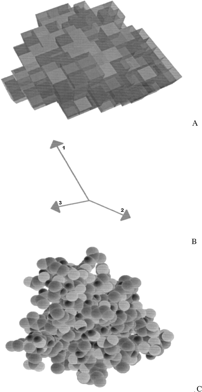
(A) Surface envelope of sevarin (PDB identification 1svr). The different shades in the SE bin the density values into three regions: light boxes, density values <0.5; medium boxes, 0.5 to 0.9; dark boxes, >0.9. (B) Principal component vectors are superimposed on a 94-atom molecular C_α model of sevarin protein domain two (1svr). (C) A molecular model representation of the same protein drawn with the graphics software Rasmol.

We use the phrase “surface envelope” to avoid confusion with two closely related concepts: the molecular surface and surface accessibility. Molecular surfaces are created by thresholding electron density data and defining the boundary between the inside and outside of a particular molecule. This is a two-dimensional data structure embedded in three dimensions, whereas the SE is a three-dimensional data structure. Surface accessibility relates how close an atom or residue sits to the molecular surface (Schmidt et al. 1998). This is a one-dimensional measurement.

Using shape information to assess the quality of a structural model is a complex task for a variety of reasons. There are two parts to the problem of creating a function capable of scoring model-envelope matches: (1) aligning the model structure to the SE and (2) generating a score from the alignment. An alignment of two objects in three dimensions consists of translating and rotating one object with respect to another. Alignment is required because of the orientation ambiguity intrinsic to shape information, in which individual atoms have not been located within the shape, and so, standard RMS fitting cannot be performed. For example, a model with an accurate molecular structure that is rotated or translated out of alignment with respect to the SE looks like an incorrect structure. Only after the model is translated and rotated so the model and the SE are aligned can a fair assessment be obtained of the model shape. Alignment is confounded by the fact that in most cases, the putative structural model typically does not have a shape that exactly matches the available shape in the SE, so there is no single correct alignment. No simple method exists for exhaustively searching possible translations and rotations for the best alignment. Lanzavecchia et al. (2001) have shown previously the value of using principle components for alignment.

Generating the score is simpler. Once a model is aligned to an SE, there are many ways of assigning a score. When atoms fall in regions of the SE with high-density values, the model should receive a higher score. One may also give models lower scores if they fail to account for all the density values present in the SE. We evaluated three different score metrics called S₁, S₂, and S₃, detailed in the Materials and Methods section. Briefly, the first score, S₁, simply counts the overlap between the model and the SE. The second score, S₂, applies a weighted average between S₁ and a global penalty factor that measures the volume of the SE not filled by atoms in the model. The third score metric, S₃, counts atoms from the model within the SE but penalizes each term in the summation if there are local regions in the SE not filled with atoms. S₃ does penalize an alignment for regions of the SE not filled, but only in regions close to atoms within the model.

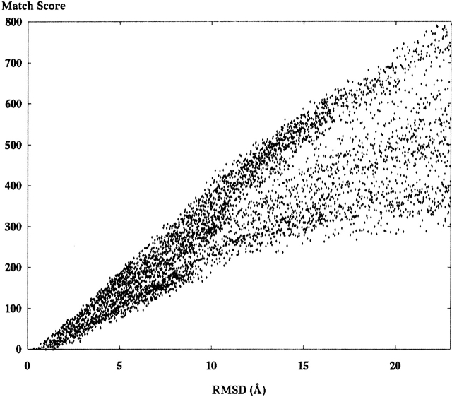
The difficulty of alignment is increased when the structural models are imperfect and do not exactly match the shape encoded in the SE. When molecular models exactly match SE shapes, there is less need to provide continuous scores to differentiate model quality based on shape information. However, our goal is to rank order a large number of models, all of which are wrong by various degrees. Poor matches between the SE shape and the model mean a variety of different alignments may all look equally correct, depending on the scoring method applied. Ideally, we would expect clear correlation between how well a given model conforms to a given shape and how close the model is to being the correct model (RMSD). Furthermore, as the RMSD increases, one would expect this correlation to slowly break down, because as models become increasingly incorrect (higher RMSD) some may match well to the available shape, whereas others may not. We would expect that at higher RMSD, a variety of model-shape matches would be possible, and so, the correlation would break down. Every model–SE pair produces a single point on such a graph, as shown in Figures 5 ▶ through 8 ▶, 9B ▶, and 12 ▶. These figures plot the RMSD versus the match score (which is high for poor matches and zero for perfect matches).

Figure 5.

A set of 6750 different models of the ribosome fragment 1ctf was scored by using S₃ against an SE derived from the crystal structure. Models were generated in 27 different groups (with 250 models each) by randomly perturbing the atoms starting in the crystal structure for each successive model in the group.

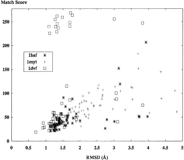
Figure 8.

Three different decoy sets were aligned and scored against an SE derived from the respective crystal structure. The first was monoclonal antibody Fab fragment (PDB code 1baf, 60 models), the second was Yellow Tuna myoglobin protein (PDB code 1myt, 58 models), and the third was monoclonal antibody Fab fragment (PDB code 1dvf, 61 models). Note the points at the top of the graph for 1dvf (which result from principal component alignment [PCA]) are discussed in Results. They result from an improper model orientation when PCA is used.

Figure 9.

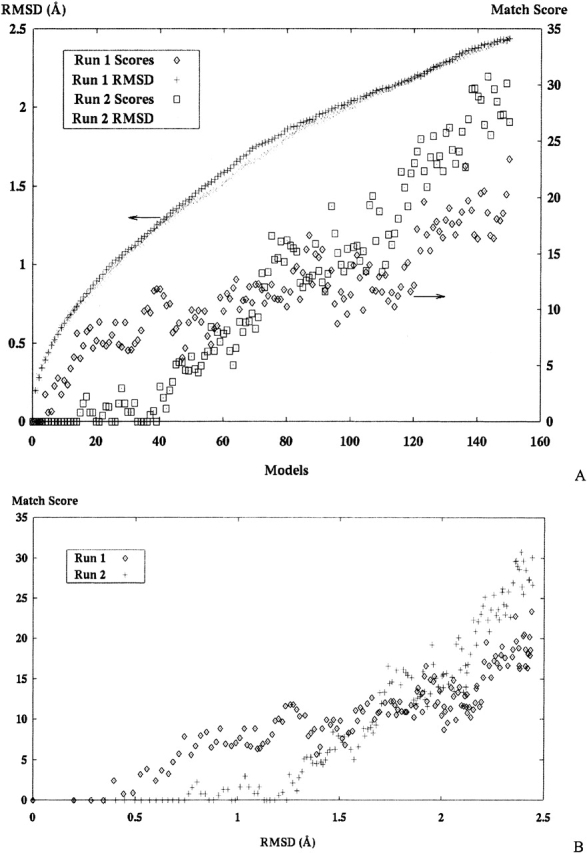
(A) Match scoring for two sets of structural models derived sequentially by random atom perturbations from the crystal structure of ribosomal protein 1ctf. Symbol x and + are the full atom RMSD of each model, and the match score for each model are boxes each model compared with the SE derived from the crystal structure. (B) The bottom graph compares the two data series from the top graph against each other for each run.

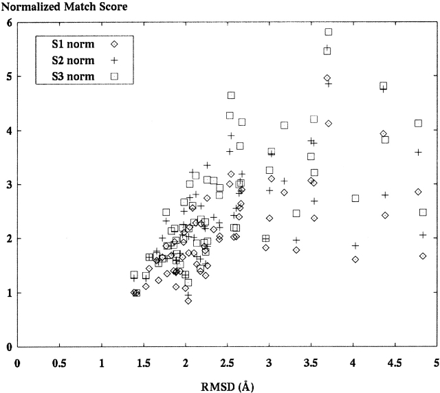
Figure 12.

This graph compares the SE match scores for decoy set models of Fab fragment 1fig using score functions S₁, S₂, and S₃. These score data have been normalized to a single structure model, arbitrarily assigned to have a normalized score of one. Note that S₃ has the greatest spread of score values.

Results

Alignment comparison

We applied our alignment methods to a large set of protein segments presented by Hodor et al. (1999), the “Hodor set.” This set of protein structures consisted of 639 distinct CATH domains selected to represent distinct structural elements. (CATH [Orengo et al. 1997] is a novel hierarchical classification of protein domain structures, which clusters proteins at four levels, class [C], architecture [A], topology [T], and homologous superfamily [H]. The original data set included 701 structures, and 62 were removed because of errors in the Protein Data Bank [PDB] files.) In each test, each protein in the Hodor set was aligned against an SE derived from the known structure. The runs assigned starting positions for each model as a random translation and orientation relative to the SE orientation. This model starting position assignment included the following four steps, performed twice in series: (1) select random direction D₁, (2) translate model 10 to 25 Å in direction D₁, (3) select random direction D₂, and (4) rotate model 30° to 330° around direction D₂. We evaluated each alignment by calculating the maximum angle observed between corresponding principal components (PCs) in the model and the SE. These tests evaluated the robustness and accuracy for each method.

PC alignment

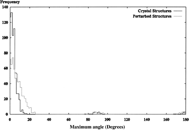
Figure 2 ▶ shows a histogram of the maximum angle between corresponding principal components for each structural model in the Hodor set after alignment by PC alignment (PCA) only. Even for correct (0 RMSD) structures, a few models incorrectly align near 90° and 180° for their maximal angle mismatch. This error occurs for models in which the PC lengths are approximately equal and the corresponding PC calculation in the SE does not have proper correspondence between the components.

Figure 2.

Each of the 639 models in the Hodor set was aligned to the crystal-derived SE using principal component alignment. Two separate sets of data are presented: one representing alignment results of original crystal structures, and the other representing results of randomly perturbed structures. Both histograms show the frequency of observed maximum angles between the principal components in the aligned model and the corresponding components in the initial orientation of the model used to generate the SE. Note that the points at 90° and 180° are misaligned, and more misalignment occurs with the perturbed structures.

These mismatches increase for models that are further from the crystal structure. In the next experiment, each structure in the Hodor set was perturbed randomly. The perturbation moved each atom three times 1 Å in each direction, resulting in structures ~1 to 2 Å RMSD from the crystal structure. Figure 2 ▶ also shows the results after alignment by PCA with several more models appearing ~90° and 180° mismatch.

Iterated closest point alignment

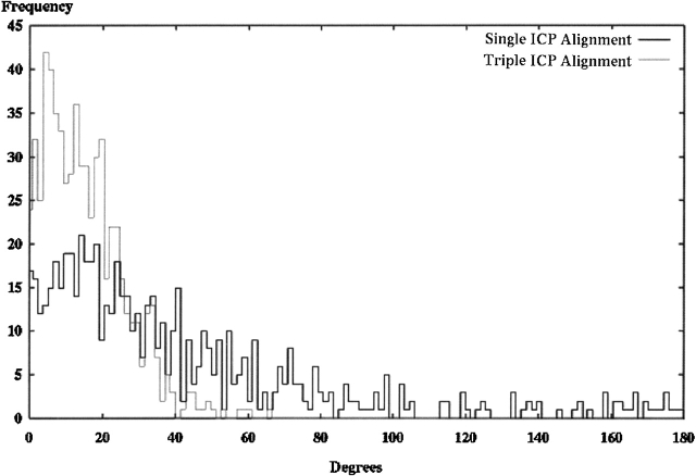
We evaluated a second method, as discussed in the Materials and Methods section, to align all models in the Hodor set with their associated SE. Figure 3 ▶ shows a histogram with the resulting angular error distribution. In this case each structure was aligned from its random starting position.

Figure 3.

Each of the 639 models in the Hodor set was aligned to the crystal-derived SE using iterated closest point (ICP) alignment. Two sets of data are presented: one with a single alignment and one with the best of three alignments. Both histograms show the frequency of observed maximum angles between principal components in the aligned model and the original crystal structure orientation. By comparison to principal component alignment, both alignments are poor; however, there are fewer misalignments at 90° and 180° using the triple ICP alignment.

Figure 3 ▶ also shows the results of using iterated closest point (ICP) alignment on the Hodor set, but in the second experiment, the best (lowest angle) result was saved from three different random starting positions. The shift of the distribution to the left was expected, as only the smallest of three trials were included in the histogram. The choice of three trials was made empirically by examination of results using many different trial runs.

Hybrid alignment

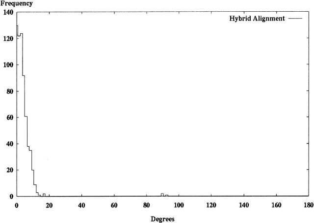
The final alignment method uses a combination of both ICP alignment and PCA. Figure 4 ▶ shows the histogram of maximal component angles for the Hodor set structures after hybrid alignment. Here we observe the elimination of structures at 180° and a significant reduction of structures at 90°. Note that this result depends on using three initial random starting orientations for each alignment result. At times we observed structures at 180°, but they were sufficiently rare that the data presented in Figure 4 ▶ represent our best expectation of alignment performance after many observations.

Figure 4.

Each of the 639 models in the Hodor set was aligned to the crystal-derived SE by using hybrid alignment described in the text in Materials and Methods. This histogram shows the frequency of observed maximum angles between principal components in the aligned model and the original crystal structure orientation.

Score function validation

We created and scored a set of molecular models from protein fragment 1ctf, the C-terminal domain of a globular protein attached to the large subunit of the Escherichia coli ribosome. Each model has 487 atoms in 68 residues, making it a small protein fragment. The set was divided into 27 different groups: Each group started with the crystal structure, and successive models in the group were generated by randomly perturbing every atom 0.6 Å in each direction. Each group has 250 models, producing a total of 6750 models. Every model was scored against SE data derived from the crystal. Figure 5 ▶ presents the match scores for each alignment between a model and an SE by using score function S₃ described in the Materials and Methods section.

Model scoring

The tests of matching models against SEs consist of aligning and scoring a series of different SE-model pairs and comparing those scores to the RMSD of the model to the correct structure. The correct structure in these cases are either the crystallographic or NMR solved structure from the PDB. The SE in each case is derived directly from the correct structure in a way that simulates experimental measurement of the SE using EM.

Three different sets of results are presented in the following three subsections, using structures derived from (1) decoy sets, (2) random perturbations, and (3) modeling trajectories. In all these cases, we apply the score functions S₁, S₂, or S₃, described later in Materials and Methods. Unless otherwise noted, the widths of the boxes in the SE are 3.7 Å. Following these three results, we present a direct comparison of the different score functions.

Decoy set scoring

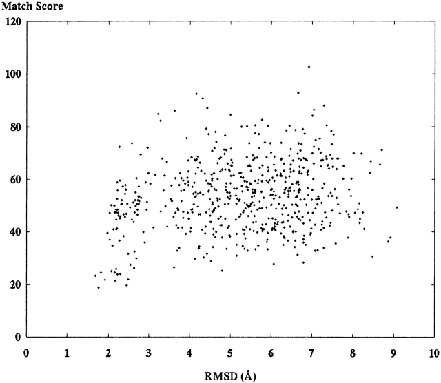
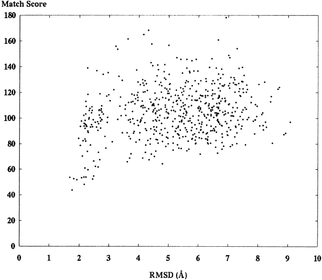
We tested 24 different decoy sets generated for the purpose of structure prediction. Table 1 presents the PDB identification of the different structures tested. A decoy set is a large number of different molecular models, each representing a different guess about the correct structure. An online resource at Stanford University called “Decoys ’R Us” provided the decoy sets (http://dd.stanford.edu). The first decoy set includes 602 different models of 1ctf as described above. Figure 6 ▶ presents a graph showing the match score using S₁ on the Y-axis and the RMSD of the model in Ångstroms (Å) on the X-axis. Figure 7 ▶ presents the same decoy set aligned and scored using S₂.

Table 1.

Protein Data Bank identification for the decoy sets used to evaluate the surface envelope alignment and scoring methods

Decoy sets [Park 1996 #161]

12 (of 24) globins: 1ash, 1emy, 1hbh-B, 1hsy, 1myg-A, 2lhb, 1bab-B, 1flp, 1hda-A, 1ith-A, 1myt, 2pgh-A

12 (of 60) immunoglobulins; 1baf, 1dbb, 1dvf, 1fai, 1fgv, 1flr, 1bbj, 1dfb, 1eap, 1fbi, 1fig, 1for

These decoys came from the Decoys ‘R Us data set available online at http: //dd.stanford.edu.

Figure 6.

A set of 602 different decoy models of the ribosome fragment 1ctf was scored against an SE derived from the crystal structure. These alignments applied score function S₁ and principle component alignment.

Figure 7.

A set of 602 different models of the ribosome fragment 1ctf was scored against an SE derived from the crystal structure. This set of scores was calculated by using S₂ from equation 3. A comparison of this graph with the one from Figure 7 ▶ reveals the improvements in model discrimination between the score functions.

The next two decoy sets come from larger immunoglobulin proteins, also derived from the Decoys ’R Us database. The first structure is a monoclonal antibody Fab fragment, 1baf in the PDB. It has 1736 atoms in 222 residues. Figure 8 ▶ presents the resulting scores of each model aligned and scored against the SE.

The second immunoglobin is also a monoclonal antibody Fab fragment with 1730 atoms in 223 residues. The PDB identification is 1dvf. These results are also in Figure 8 ▶.

The final decoy set contains structures of yellow tuna myoglobin with PDB identification 1myt. This is an α-helical structure with 1092 atoms and 146 residues. These results are also in Figure 8 ▶.

Random perturbation

Another way to generate a set of models is to take the correct structure and randomly perturb atoms. Each atom is randomly moved 1.0 Å in each direction from its current position to determine its position in the next model in the set. Van der Waals interactions are ignored. Clearly, these models are not indicative of the structural properties observed in nature, nor do they represent reasonable guesses about correct structures. Models generated by small random perturbations provide a smooth and continuous series of models at RMSD ranges very close to the correct structure. The decoys tested in the first two experiments described above do not come closer than a few Ångstroms RMSD to the correct structure.

The results of two randomly generated model sets are presented in this section. The correct structure in both cases is the ribosomal protein 1ctf. Results of the both random model sets are presented in Figure 9 ▶.

Trajectory analysis

A final source of molecular models for alignment tests includes models created during structural optimization computations (Williams et al. 2001). The set of models used for this test were created from each cycle of a distance-based calculation of the sevarin domain 1svr, a 94-atom structure. Figure 10 ▶ presents these results in three graphs; the top shows the progression of the modeling run as model moves toward the correct structure, the middle graph presents the score for each model from the set against the SE, and the bottom presents the RMSD of each model versus the match score.

Figure 10.

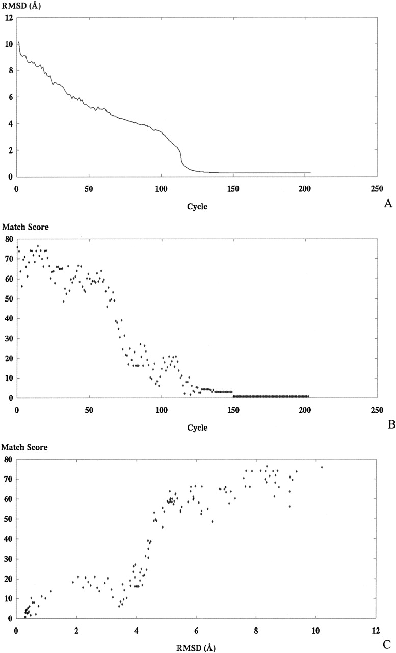
(A) RMSD for each model in the set. The ordering of the set is the same as that observed during the modeling run, from left to right. (B) Score for each model in the set. (C) Combines the data presented in the top two and plots score versus RMSD for each model in the set.

EM data

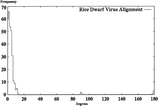
To ensure that our results on synthetic data sets translated into good performance on experimental data sets of the type we targeted, we applied hybrid alignment to EM density data shared with us by Dr. Hong Zhou et al. from a published study (2001) on the structure of the P8 trimer in the rice dwarf virus. These data were transformed into an SE by linearizing the data and thresholding it to a range of (0,1). Figure 11 ▶ shows the results of 300 sequential tests of the hybrid alignment. As no published molecular structure exists for P8, we made a surrogate model by using the points in the experimental SE with values >0.25 to act as the molecular model. Thus, the most dense locations in the experimental density map were assigned unlabeled atoms, and we used these as a surrogate structural model, lacking a high-resolution model. In each test, this model for the P8 protein was randomly rotated and translated away from its initial position, and we applied the hybrid alignment algorithm to determine how accurately we could realign the model to the initial orientation using our alignment algorithm.

Figure 11.

This histogram shows the frequency of observed maximum angles between principal components from 300 hybrid alignment runs of shape data measured by electron microscopy for a single trimer of protein P8 of the rice dwarf virus outer capsid. For each test, the initial model was rotated and translated to a random position, and the hybrid alignment algorithm was applied to reposition the data set against the initial, reference orientation.

Score function comparison

We perform a direct comparison of score functions for a subset of structures to determine the best method to apply for modeling. The structure used for this comparison has PDB identification 1fig, a 1721-atom structure. 1fab is a Fab fragment from immunoglobulin G1. A set of 63 different decoys were aligned by using the hybrid alignment method and all three score functions, the results of which are shown in Figure 12 ▶. The data are normalized to a single (arbitrary) structure assigned a Y-axis value of one. All other scores in each set are scaled for comparison. From these data we calculate the correlation coefficient for each score function as 0.614, 0.681, and 0.677, respectively, for score functions 1, 2, and 3. In addition, there are significant differences in running times between the different score functions. A sample of the run times (in seconds) for scoring runs of 1ctf were 2195, 5515, and 3202, applying score functions 1, 2, and 3, respectively. This means that S₂ exhibits a time ratio of ~2.5 times the run time of S₁ and S₃ has a ratio of ~1.45. Times come from runs on an Intel PII-450 computer (Intel Corp.).

Discussion

We have presented a set of methods to align and score molecular models to SEs. Two different alignment methods and three different scoring functions were evaluated and confirmed on shape data measured by EM reconstruction. The current data show the best results differentiating models based on shapes using the scores S₃ defined in equation 4 in the Materials and Methods section below and the hybrid alignment method.

We observed the expected behavior of match scores in almost all of the envelope matching results. As RMSD increases, the value of the SE would decrease in its ability to discriminate model shapes. Above some RMSD value (we call this the “fall-over point”), the minimum match scores became basically flat. However, depending on the scale on the Y-axis, the actual RMSD value above which shapes become irrelevant varies depending on the structure in question. It was surprising to note that the shape of the graphs differed somewhat between the decoy set matching and the envelope matching done on random perturbation models. Most notably, the random perturbation (Fig. 5 ▶) exhibits a fall-over point at ~10 Å. Models with RMSD above this value show lower correlation with envelope score. Said another way, we observed that models in the random set that were >10 Å RMSD showed high correlation with envelope score. The surprise was that for decoy set scoring, this value was much lower, ~2.5 to 3.5 Å. This can be seen in Figure 8 ▶. One possible explanation for this difference is the clear difference in methods used to generate models in the two different sets. The decoy set models are more tightly packed, resulting in better matches to the correct shape at lower RMSD values.

Comparing the alignment methods highlights the problems with both PCA and ICP used alone. PCA alone occasionally fails even in the alignment of crystal structure models with SE shapes derived from the same models due to incorrect correspondences between PCs in the model and the SE. The frequency of these incorrect correspondences increases for models further from the correct structure. Examples of this effect appear at the top of Figure 9 ▶, showing scores for structure 1dvf. The PCA algorithm fails because incorrect PC matching occurs. This happens because in some models, the rank ordering of PC vectors may change causing a 90 or 180 flip of the model with respect to the SE. This problem gets worse when the ratio of longest to shortest principle component approaches one, and we found ratios generally <1.2 to 1.3 problematic. An abrupt orientation shift of this magnitude would cause critical failures during modeling. The main failure of ICP comes from its inability to move models all the way to an accurate alignment: an optimization local minimum. The degree of failure in ICP is highly dependent on the starting position of the model, and taking multiple ICP trials mitigates much of the issue. The clear winner in alignment is the hybrid model, applying strengths from both techniques. With the hybrid technique, the several successive ICP trials identify a close starting points for assigning accurate PC correspondences.

Our results demonstrate the power of shape information to differentiate correct structures from incorrect ones. Although the results from the 1ctf decoy set in Figure 6 ▶ are mediocre, slightly better results are seen by using a more complex score function in Figure 7 ▶. With the exception of a few models in the lowest RMSD, the models are effectively not differentiable using our scoring methods. This is partly because PC with similar magnitudes in the 1ctf structure confounds the PCA. It is also notable that the 1ctf structure is highly globular, and regardless of the accuracy of the alignment, the shape information from the SE does not add significantly to our understanding of the 1ctf structure. Other structures with more elongated shapes have more information about their structure encoded in their shape.

The alignment and scoring of other decoy sets shows clear ability of our methods to distinguish low RMSD models from higher ones. Results in Figure 8 ▶ for structures 1baf, 1dvf, and 1myt show expected behavior in the RMSD versus match score curves. These results are best with the more accurate score function S₃ and hybrid alignment and indicate that using shape information for discrimination may be very valuable for prospective modeling. These promising results lead directly to the application of shape information in creating novel biomolecular models.

Materials and methods

Surface envelopes

The implementation of SEs and the algorithms for aligning and scoring were coded by using C++. The SE data used in these tests were generated from solved crystal structures to approximate data that could be measured experimentally. Density values for each box in the SE correspond to the amount of atom volume that overlaps the box. A Monte Carlo method was used to determine the contributions of each atom to the different density values in the SE. For each atom, 100,000 points were selected at random within the Van der Waals radius from the atom center. The proportion of the points falling in each box was added to the corresponding density value. After this process, all boxes with density values greater than 1 were set to 1.

Scoring

Matching a model to an SE involves two steps. First, the model and SE must be registered in three-dimensional space. We present two different methods below and a hybrid method that uses parts of both alignment methods. The second step occurs once the registration is complete: A scoring function is applied to determine how well the shape of the model and the SE agrees. We call the resulting score the “match score.” The section Scoring Envelope Matches below presents three different scoring functions and the relative merits of each for different purposes.

PC alignment

PCs of a set of points are a set of three orthogonal vectors. The direction of the longest and shortest PC vectors corresponds to the direction with the greatest and smallest variance of point positions from the center of mass (Mortenson 1995). Given the first two components, the direction of the middle component is determined by the right hand rule. The magnitude (length) of each of the three vectors corresponds to the amount of deviation from the center of mass by the complete collection of points in the vector direction. The calculation of PC is performed by eigenvector decomposition on the square symmetric matrix of deviations, M,

(1)

where d_x is the deviation of a given point from the center of mass in the x direction, with similar definitions for d_y and d_z. The three eigenvectors of this matrix define the direction of the PCs, and the eigenvalues are the PC lengths. For a set of atoms, the PCs are calculated by assuming each atom is a single point. For SE, each box in the three-dimensional grid is treated as a point, and d_x, d_y, and d_z in equation 1 are weighted by the density number in each box. Figure 1 ▶ shows an example of PC vectors superimposed on a molecular model. The model is a C_α representation of sevarin protein domain two (PDB ID 1svr). The alignment uses PC vectors from both the model and the SE. The two structures are superimposed at their center of mass. The atoms in the model are all rotated to bring the first and third (longest and shortest) PC vectors into collinear alignment.

For PCA to work, the lengths of the three vectors must be distinct. A situation in which the components are all the same, such as a sphere, or two of the components are equal, such as a cylinder, introduces rotational symmetry. More precisely, the greater the ratio of magnitude between the longest and shortest component in the correct structure and the SE, the easier it is to ensure that the correct components are aligned in any particular model.

ICP alignment

This alignment method applies an adaptation of the ICP algorithm (Besl and McKay 1992). ICP is a general-purpose method for accurate registration of three-dimensional shapes. The algorithm has three basic steps: (1) compute closest points in the SE for every atom in the model, (2) compute the closed-form translation and rotation that aligns the corresponding model–SE point pairs as well as possible to minimize a distance-based score metric, and (3) apply the translation and rotation to the model.

The algorithm iterates the previous three steps until either the error from the score metric decreases below a threshold, or the same correspondence points are regenerated, leading to a null transformation of the model. The choice of scoring function for determining the transform affects both the speed and the accuracy of convergence. We apply least-squares minimization of distances to minimize the RMSD between all current correspondences.

Another variation to the ICP algorithm includes the addition of a maximum distance cutoff for which no correspondence is assigned. This helps the algorithm to determine the best fit for models that do not fit the SE shape exactly, by leaving out points that fit poorly. We restrict the point correspondences between the model and the SE to unique points in each data set. Thus, each point in the model and the SE is assigned a maximum of one correspondence to a point in the other data structure. The number of points in the SE is much greater than that of the molecular model, so this results in picking unique SE points for each atom point in the model. The algorithm has an observed dependence on the relative starting position of the model with respect to the SE. The method typically does not make significant rotations and translations after the first or second alignment iteration. Each step after the first few is an incremental step to align the two structures.

Hybrid alignment

The early results of both PC and ICP prompted the investigation of a hybrid method of model–SE alignment that took some of the positive features of both methods. The PC–ICP hybrid alignment method applies the following steps:

1. Perform ICP alignment three times, randomizing the position and orientation of the model wrt: SE after each alignment. Select final position from ICP with lowest distance metric.

2. Translate the model to align the center of mass of the model and the SE.

3. Align using the PC method, but assign component correspondence based on the closest component defined by the current model position. (In this case, closest is defined by the smallest angle between components.)

4. Iteratively adjust the resulting alignment to minimize the score by applying small translations and rotations based on the position of atoms outside the SE. These adjustments move atoms distances on the order of box widths in the SE.

Scoring envelope matches

We present three different methods for assigning a score to a model aligned against an SE. The first method defines the total score, S₁, with

(2)

where D_i is the density value from SE at the location of atom i. This score method is fast and atom-centric because all parts of the score function can be attributed to specific atoms. We report a final match score as the difference between the maximum possible score and the calculated value S₁, providing a zero score for a perfect match and increasing values for imperfect matches.

The second scoring method includes a penalty to the total score for regions of the SE not filed with atoms. We define S₂ with

(3)

where penalty factor P_j equals zero for each box j in the SE that contains an atom, and equals the density value in the box (a value from zero to one) if no nearby atom can account for the atom density expected in box j. The variables α₁ and α₂ are adjustable scaling factors. Two factors make this match scoring function significantly more computationally intensive to calculate than S₁. First, the magnitude of m, the number of boxes in the SE, is significantly greater than n, typically by an order of magnitude. The second difficulty is that the implementation of atoms within the model tracks their positions as points. The SE data structure uses boxes on the three-dimensional grid to store the sum of atom densities. To accurately calculate the value of P_j, all adjacent boxes in the SE (the 26 neighbors of P_j) must be checked for atoms close to box j, because atoms with positions near a box edge attribute density to the SE in both boxes adjacent to that edge. S₂ is not an atom-centric scoring method. The elements included in the second summation can no longer be attributed to any particular atom thus making it potentially less useful as part of an atom-based modeling method.

The third scoring function includes a penalty factor similar to S₂ but also maintains all parts of the score function as attributable to particular atoms. We define S₃ with

(4)

where P_i is now a penalty term calculated for each atom. Similar to the above penalty, S₃ reduces the score for regions of the SE not filled with atoms. In this case, P_i is the sum of penalty term P_j defined above, but calculated over SE boxes adjacent to the box containing atom i. This does not completely account for large sections of the SE not covered by atoms, but it does more accurately represent the shape matching compared with S₁.

References

- Besl, P.J. and McKay, N.D. 1992. A method for registration of 3D shapes. IEEE Transactions on Pattern Analysis and Machine Intelligence 14 239–256. [Google Scholar]
- Branden, C. and Tooze, J. 1999. Introduction to protein structure. Garland Publishing, New York.
- Chiu, W., Baker, M.L., Jiang, W., and Zhou, H. 2002. Deriving folds of macromolecular complexes through electron cryomicroscopy and bioinformatics approaches. Curr. Opin. Struct. Biol. 12 263–269. [DOI] [PubMed] [Google Scholar]
- Frank, J. 1996. Three-dimensional electron microscopy of macromolecular assemblies. Academic Press, New York.
- Hodor, P.G., Caruana, R., Sassaman, E., Buchanan, B.G., and Rosenberg, J.M. 1999. Examination of amino acid sequence rules for α helix pairing in proteins. Poster session, International Conference on Intelligent Systems for Molecular Biology, Heidelberg, Germany.
- Kaiushina, R.L., Izotova, T.D., Mogilevskii, L.I., Shmakova, F.V., and Khurgin, I.I. 1985. Study of the structure of immunoglobins by small-angle x-ray diffraction, I: The structure of IgMCep in solution. Bioorg. Khim 11 753–761. [PubMed] [Google Scholar]
- Lanzavecchia, S., Cantele, F., and Bellon, P.L. 2001. Alignment of 3D structures of macromolecular assemblies. Bioinformatics 17 58–62. [DOI] [PubMed] [Google Scholar]
- Mortenson, M.E. 1995. Geometric transforms. Industrial Press, New York.
- Orengo, C.A., Michie, A.D., Jones, S., Jones, D.T., Swindells, M.B., and Thornton, J.M. 1997. CATH: A hierarchic classification of protein domain structures. Structure 5 1093–1108. [DOI] [PubMed] [Google Scholar]
- Sali, A. and Blundell, T.L. 1993. Comparative protein modelling by satisfaction of spatial restraints. J. Mol. Biol. 234 779–815. [DOI] [PubMed] [Google Scholar]
- Schmidt, J.P., Chen, C.C., Cooper, J.L., and Altman, R.B. 1998. A surface measure for probabilistic structural computations. Proc. Int. Conf. Intell. Syst. Mol. Biol. 6 148–156. [PubMed] [Google Scholar]
- Simons, K.T., Bonneau, R., Ruczinski, I., and Baker, D. 1999. Ab initio protein structure prediction of CASP III targets using ROSETTA. Proteins 3 171–176. [DOI] [PubMed] [Google Scholar]
- Urbanke, C. and Ziegler, B. 1980. Complete evaluation of sedimentation velocity experiments in the analytical ultracentrifuge. Fres. Z. Anal. Chem. 301 139–140. [Google Scholar]
- Williams, G.A., Dugan, J.M., and Altman, R.B. 2001. Constrained global optimization for estimating molecular structure from atomic distances. J. Comp. Biol. 8 523–547. [DOI] [PubMed] [Google Scholar]
- Zhou, Z.H., Baker, M., Jiang, W., Dougherty, M., Jakana, J., Dong, G., Lu, G., and Chu, W. 2001. Electron cryomicroscopy and bioinformatics suggest protein fold models for rice dwarf virus. Nat. Struct. Biol. 8 868–873. [DOI] [PubMed] [Google Scholar]