Optimal bundling of transmembrane helices using sparse distance constraints

Abstract

We present a two-step approach to modeling the transmembrane spanning helical bundles of integral membrane proteins using only sparse distance constraints, such as those derived from chemical cross-linking, dipolar EPR and FRET experiments. In Step 1, using an algorithm, we developed, the conformational space of membrane protein folds matching a set of distance constraints is explored to provide initial structures for local conformational searches. In Step 2, these structures refined against a custom penalty function that incorporates both measures derived from statistical analysis of solved membrane protein structures and distance constraints obtained from experiments. We begin by describing the statistical analysis of the solved membrane protein structures from which the theoretical portion of the penalty function was derived. We then describe the penalty function, and, using a set of six test cases, demonstrate that it is capable of distinguishing helical bundles that are close to the native bundle from those that are far from the native bundle. Finally, using a set of only 27 distance constraints extracted from the literature, we show that our method successfully recovers the structure of dark-adapted rhodopsin to within 3.2 Å of the crystal structure.

Integral membrane proteins are essential components of the cell membrane that participate in many important cellular processes such as energy transduction, cell signaling, mediation of senses such as vision, cell intoxication, and pathogenesis, and immune recognition. Their significance is emphasized by the fact that approximately one-third of the proteins encoded for by a typical genome are membrane proteins (Buchan et al. 2002). Furthermore, at least 70% of current pharmaceuticals are thought to act on membrane proteins (Wilson and Bergsma 2000). Despite their obvious importance, to date, the structures of fewer than 75 integral membrane proteins have been solved (see White 2003 and references therein), and this number includes redundant structures across species. This is a vast contrast to the over 25,000 soluble proteins whose structures have been solved using X-ray crystallography and NMR. Reasons for the slow progress in the structural analysis of membrane proteins include the instability of membrane proteins in environments lacking phospholipids, their tendency to aggregate and precipitate, and protein abundance, expression, and purification issues. These characteristics highlight why the application of standard structure determination methods to membrane proteins is nontrivial.

Given the nature of the difficulties in generating high-resolution structural data from methods such as X-ray crystallography and NMR, it is unlikely that these experimental techniques will yield a significant increase in the number of solved membrane protein structures in the near future. As an alternative approach, the focus here is on modeling transmembrane proteins using a set of sparse distance constraints, thus leveraging the many recent advances in techniques for measuring distances within a protein. Such methods include chemical cross-linking combined with mass spectrometry (Bennett et al. 2000; Rappsilber et al. 2000; Young et al. 2000; Back et al. 2002; Taverner et al. 2002; Dihazi and Sinz 2003; Kruppa et al. 2003; Novak 2003; Schilling et al. 2003), site-directed spin labeling combined with electron paramagnetic resonance (SDSL-EPR) (Rabenstein and Shin 1995; Farrens et al. 1996; Hustedt et al. 1997; McHaourab et al. 1997; Steinhoff et al. 1997; Hustedt and Beth 1999; Altenbach et al. 2001; Borbat et al. 2001; Liu et al. 2001; Persson et al. 2001; Radzwill et al. 2001; Brown et al. 2002; Perozo et al. 2002; Hubbell et al. 2003), disulfide bond formation mapping (Cai et al. 1999, 2001; Yu et al. 1999), and fluorescence resonance energy transfer (FRET) (Matyus 1992; Hillisch et al. 2001; Klostermeier and Millar 2001; Parkhurst et al. 2001; Rye 2001; Szollosi et al. 2002; Sekar and Periasamy 2003). These methods produce low-to-moderate resolution structural data that can be used in conjunction with computational predictions, such as structural rules derived from helix–helix interactions in known structures (Bowie 1997, 1999), to determine a transmembrane protein structure to moderate resolution.

The modeling challenge of constructing a transmembrane helical bundle that is consistent with a set of low-to-moderate resolution experimental constraints can be simplified by considering some of the relative characteristics of a transmembrane protein. The low dielectric environment of a lipid bilayer favors the formation of regular secondary structural elements (SSE), such as helices and β-sheets, by increasing the strength of hydrogen bonds (White and Wimley 1999; Kim and Cross 2002). The thermodynamic disadvantages of transferring nonhydrogen bonded peptides from a water to a lipid environment (+5 kcal/mole per H-bond; Engelman et al. 1986) imply that transmembrane proteins fold and assemble in a multistage process (Jacobs and White 1989; Popot and Engelman 1990). We assume the two-stage model (Popot and Engelman 1990), and describe the construction of transmembrane protein models as two separate tasks: (1) defining the transmembrane SSEs, and (2) determining their relative orientations or packing.

Although not a solved problem, transmembrane spanning SSEs can be accurately predicted from sequence information using widely accepted methods such as sliding-window hydrophobicity analysis (Rose 1978; Jayasinghe et al. 2001a, b). However, subsequent prediction of the association of these helices into the final transmembrane protein fold is not well established. Structural constraints imposed by the lipid bilayer on transmembrane SSEs do limit the number of possible membrane protein folds (White and Wimley 1998), and several ab initio and potential based computational approaches for predicting interhelical packing have been proposed (Bowie 1997, 1999; Nikiforovich et al. 2001; Dobbs et al. 2002; Fleishman and Ben-Tal 2002; Vaidehi et al. 2002; Kim et al. 2003).

Several of these approaches incorporate experimental data into their models. For example, Nikiforovich et al. (2001) use the similarity between the X-ray structures of bacteriorhodopsin and rhodopsin to estimate helix packing in the membrane plane. Specifically, the intersections between the helical axes and the membrane plane are fixed at values derived from the two X-ray structures. Vaidehi et al. (2002) orient each helical axis of the helical bundle according to the 7.5 Å electron density map of rhodopsin. Herzyk and Hubbard (1995) developed an automated approach to modeling seven helix transmembrane receptors using a combination of data from electron microscopy, neutron diffraction, mutagenesis, chemical cross-linking, site-directed spin labeling, disulfide mapping, FTIR difference spectroscopy, solid-state ¹³C NMR, semiempirical calculations on ligand–protein interaction, multiple sequence alignment, and hydrophobicity. Using a potential function designed to constrain model structures to satisfying these data, they built a model structure of bacteriorhodopsin that was within 1.87 Å RMSD of the structure determined by electron microscopy. By combining several types of data, they have laid the groundwork for developing scoring functions that constrain helical bundles using experimental data. In this work, we take a similar approach; however, rather than using data taken from a variety of experiments, we develop a function based solely on distance constraints and data mined from structures in the PDB.

In this article, we describe a two-step approach to modeling the transmembrane spanning, helical bundles of integral membrane proteins using sparse distance constraints. Because many of the known membrane protein structures are all α-helical, we limit our discussion to modeling helical bundles. The method is as follows:

Step 1. Search the conformational space of membrane protein folds to find those matching a given set of distance constraints (Faulon et al. 2003);

Step 2. Refine the helical bundles from Step 1 using a Monte Carlo simulated annealing protocol designed for local minimization of a custom penalty function referred to as Bundler.

The Bundler function scores a helical bundle based on its consistency with the structural features of known transmembrane bundles as well as with distance constraints from experimental methods such as chemical cross-linking, NMR, FRET, and EPR. In the following sections the Bundler penalty function is described in detail and validated across a set of six known transmembrane protein structures to show that it is capable of distinguishing between structures close to and far from the native structure. We also demonstrate that our two-step approach can recover the transmembrane helical bundle of the dark-adapted rhodopsin structure (1f88) to within 3.2 Å RMSD of the native structure using only 27 experimental distance constraints gathered from the literature.

Results

We begin this section by presenting a statistical analysis of a set of nonredundant helical transmembrane proteins. This is followed by a description of the penalty function, referred to as Bundler, and validation of the penalty function as a tool to differentiate near native helical bundles from those far from the native bundle is then described. Using a set of six membrane proteins crystal structures the penalty function is validated by showing that helical bundles with lower RMSD from the X-ray structure score lower than those with higher RMSD. Last, we demonstrate the method on the structure of dark-adapted rhodopsin using a set of distance constraints taken from the literature.

Statistical analysis of membrane protein structures

The set of 14 membrane proteins listed in Table 1, with all-α-helical transmembrane domains, was examined to extract statistical information about their helix packing distances, angles, and number of nearest neighbors. Because the structure of the individual helices comprising the helical bundle is not likely to be known, we assumed that in most cases the bundle will initially be modeled using idealized helices and concluded that collecting statistics on an idealized set of the 14 transmembrane proteins would result in the most useful statistical parameters for the scoring function. Idealized representations of the 14 proteins were constructed by superimposing perfect α-helical structures of the appropriate lengths onto the helices in the transmembrane domains. The Cα level RMSD between the individual idealized helices and their corresponding helices from the PDB structure ranged from 0.56 Å (1PRC, 17 aa) to 4.07 Å (1QLAC, 35 aa), while across all helices of the transmembrane domain, the Cα level RMSDs ranged from 1.15 Å (1FQY, 136 aa) to 2.37 Å (1QLAC, 160 aa).

Table 1.

Structures used for statistical characterization of transmembrane protein bundles

PDB ID	Name	Number of AAs
1BL8	KcsA potassium channel	388
1C3W	Bacteriorhodopsin	222
1E12	Halorhodopsin	239
1EHK	Ba3 cytochrome c oxygenase	743
1EUL	Calcium ATPase	994
1EZVC	Cytochrome bc1 complex	385
1F88	Rhodopsin	338
1FQY	AQP1—aquaporin water channel	226
1FX8	GlpF—glycerol facilitator channel	254
1JGJ	Sensory rhodopsin II	217
1MSL	McsL mechanosensitive channel	545
1OCC	aa3 cytochrome c oxidase	1780
1PRC	Photosynthetic reaction center	605
1QLAC	Fumerate reductase complex	254

Statistics collected on the 14 idealized representative structures are listed in Table 2. Means and standard deviations were calculated for the distances between the centers of mass for consecutive helices (δ_COM,cons), distances between the centers of mass for all helical pairs (δ_COM), the minimum approach distance of the helical axes for consecutive helices (δ_min,cons), the minimum approach distance of all helix axial pairs (δ_min), the packing angle of helical axes (θ_pack), and the number of helical neighbors (n_neigh) with a minimum pairwise approach distance less than 15 Å. Note that in Table 2, N indicates the sample size.

Table 2.

Statistics describing transmembrane protein helical bundles

Statistic	μ	σ	N
δCOM,cons	12.8 Å	5.3 Å	86
δCOM	18.6 Å	7.32 Å	336
δmin,cons	10.7 Å	5.2 Å	86
δmin	16.3 Å	7.4 Å	336
θpack	30.9°	16.4°	336
nneigh	3.4	1.4	102
ρpack	37.1	2.5	16

All statistics were calculated on the set of proteins listed in Table 1 with the exception of the packing density, ρ_pack, which was calculated on the proteins listed in Table 2.

Fleishman and Ben-Tal have suggested that short loops, less than 20 amino acids, play an important role in determining the packing of helices in membrane protein structures (Fleishman and Ben-Tal 2002). Hence, in addition to experimentally determined distances, we include distances generated by correlating loop lengths to helix-end to helix-end distances. Using our set of 14 helical membrane proteins, we correlated the helix-end to helix-end distances with the number of amino acids in the loop connecting the two helices (Fig. 1 ▶). Across the span of loop lengths, this correlation is quite low (R² = 0.4). However, dividing this sample into a group with loops containing seven or fewer amino acids (R² = 0.8) and loops with eight or more amino acids (R² = 0.2) allowed us to develop a set of guidelines for deriving helix-end to helix-end distance constraints given the number of amino acids in the loop. The least squares line through the points with seven or fewer amino acids is, where D is the helix-end to helix-end distances and x is the number of amino acids. Using a 95% confidence interval around this least squares line and the minimum and maximum distances for loops with eight or more amino acids, we obtain the following upper (UB) and lower (LB) bounds for distance constraints between helix ends:

Figure 1.

Correlation of helix-end to helix-end distance with number of amino acids in the loop. Statistics are for the 36 helix-end to helix-end distances extracted from the set of 14 nonredundant structures given in Table 1.

(1)

For loops ranging from 4 to 8 residues the upper bounds are 13.5 Å, 15.2 Å, 16.8 Å, 18.1 Å and 20.1 Å, respectively, which compare well to the values of 14.7 Å, 15.7 Å, 18.2 Å, 18.2 Å and 20.7 Å reported by Herzyk and Hubbard (Herzyk and Hubbard 1995).

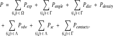
Penalty function

The Bundler penalty function incorporates distance constraints determined via experimental methods such as chemical crosslinking, dipolar EPR, FRET, and NMR. Bundler assesses a possible helical bundle and assigns it a score reflecting, in part, its degree of consistency with a set of experimental distance constraints. Given a large enough experimental distance constraint set, such a function would require no additional considerations; however, measuring distances in membrane proteins is difficult, so it is likely that only a sparse number of distance constraints will be available. Moreover, it is expected that the available distances will not be error free. Therefore, to improve its viability, Bundler also includes penalties for violating a set of helix packing parameters determined by the analysis of a set of membrane protein structures from the PDB. Note that although after the first step of the overall modeling procedure only helical bundles satisfying the distance constraints remain, it is still necessary to include a distance constraints penalty to avoid allowing the bundle to deviate far from experimental results in favor of the structure survey-based constraints. The total penalty, P, is thus the sum of a distance constraint penalty and the structure-based penalties:

(2)

Distance constraints penalty (P_dist)

Distance constraints provide moderate resolution structural information and are a crucial component in our modeling of helical membrane proteins (Faulon et al. 2003). Bundler penalizes structures that violate distance constraints according to a “soft” square well potential defined as

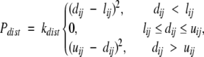(3)

where l_ij and u_ij are the lower and upper limits on the distance between atoms i and j, respectively; d_ij is the distance between atoms i and j in the current bundle; and k_dist is a force constant and was set to 500.

Structure-based penalties

The structure-based piece of the scoring function consists of penalties for helical bundles with packing angles, packing distances, and/or packing densities outside the ranges determined from analysis of a nonredundant set of helical transmembrane protein structures. It also incorporates a van der Waals repulsive potential, a “compactness” penalty for having too few neighboring helices, and a penalty for unlikely side-chain interactions. Summing these terms gives the total structure-based penalty:

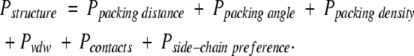(4)

Below, we describe each of the terms of equation 4 in detail.

Packing distance penalty (P_pdist)

The mean distance between the centers of mass of consecutive helices, as derived from the set of 14 nonredundant helical transmembrane protein structures (Table 1), is 12.8 ± 5.3 Å, while the mean distance between consecutive helical line segments is 10.7 ± 5.2 Å. A packing distance penalty is applied if either the centers of mass of the consecutive helices or the minimum distance between the two helical axes falls outside 1.5 standard deviations of their respective mean. The packing distance penalty is defined as a soft square well potential,

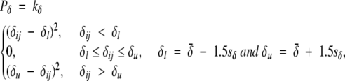(5)

where δ̄ and s_δ are the mean and standard deviation of the interhelical distance, respectively; δ_ij is the distance between the centers of mass of helix i and helix j in the current structure; and k_δ is a force constant, which we set at 50. The packing distance term is summed over the set of distinct helical pairs.

Packing density penalty (P_pdens)

Packing density is defined as the ratio of atomic volume to solvent accessible volume (Richards 1974). Because average protein packing density does not vary significantly with secondary structure class (Chothia 1975), we increased our sample size for calculating packing density statistics by analyzing a nonredundant set of 28 α-helical and/or β-strand-containing membrane proteins (Table 3) from which the mean backbone packing density was 37.1 ± 2.5. Structures with a packing density greater than 1.5 standard deviations away from the mean are penalized using a soft square well potential,

Table 3.

Packing density statistics

PDB ID	Number of AAs	Name	TM class	Packing density
1BL8	388	KcsA potassium channel	α	37.0
1BXW	172	OmpA	β	37.0
1C3W	222	Bacteriorhodopsin	α	38.0
1E12	239	Halorhodopsin	α	38.0
1EHK	743	ba3 cytochrome c oxygenase	α	38.0
1EK9	423	TolC outer membrane protein	β	37.0
1EUL	994	Calcium ATPase	α	37.0
1EZVC	385	Cytochrome bc1 complex	α	37.0
1F88	338	Rhodopsin	α	37.0
1FEP	669	FepA	β	37.0
1FQY	226	AQP1—aquaporin water channel	α	36.0
1FX8	254	GlpF—glycerol facilitator channel	α	38.0
1JGJ	217	Sensory rhodopsin	α	38.0
1LGH	198	Light harvesting complex	α	37.0
1MAL	421	Maltoporin	β	37.0
1MSL	545	MscL mechanosensitive channel	α	35.0
1OCC	1780	aa3 cytochrome c oxidase	α	37.0
1PHO	330	PhoE	β	37.0
1PRC	605	Photosynthetic reaction center	α	36.0
1QD5	257	OMPLA	β	37.0
1QJ8	148	OmpX	β	39.0
1QLAC	254	Fumerate reductase complex	α	37.0
2FCP	705	FhuA	β	37.0
2MPR	421	Maltoporin	β	37.0
2OMF	340	OmpF	β	38.0
2POR	301	Porin	β	38.0
3LKF	292	LukF	β	37.0
7AHL	293	α-hemolysin	β	36.0

(6)

where ρ̄ and s_ρ are the mean and standard deviation of the packing density, respectively; and k_ρ is a force constant, which we set at 500.

Packing angle penalty (P_angle)

The helix packing angle score penalizes structures in which the angle between the helical axes of consecutive pairs of helices is outside 1.5 standard deviations of the average angle. The mean packing angle between consecutive pairs of helices, calculated over the nonredundant set of 14 helical transmembrane proteins in Table 1, is 30.9 ± 16.3 Å. Packing angle violations are penalized according to a soft square well potential,

(7)

where θ̄ and s_θ are the mean and standard deviation of the packing angles, respectively; and θ_ij is the angle between helix i and helix j. The force constant is equal to 5. The packing angle penalty is summed over the set of consecutive helical pairs.

van der Waals repulsion (P_vdw)

To avoid overlapping helices, we include a van der Waals potential. Because our helix bundling is done at the Cβ level of atomic detail, we use only the van der Waals repulsive function (Brünger et al. 1998)

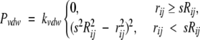(8)

to prevent interhelical clashes. Here, s is a predetermined van der Waals scaling factor and was set to 1; r_ij is the distance between Cβ atoms i and j; R_ij is the distance at which atoms i and j begin to repel each other; and k_vdw is a weighting constant and is set at 5. This piece of the penalty function is summed over the set of all pairs of Cβ atoms, and for computing efficiency, we consider only Cβ–Cβ clashes.

Contact penalty (P_contact)

Our analysis of the 14 membrane proteins listed in Table 1 revealed that the helices are usually in contact with at least two neighbor helices. To guarantee that this is the case in our candidate helical bundles, we apply a simple linear penalty to any structure containing a helix that is not in contact with at least two neighbors and define a contact penalty as:

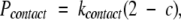(9)

Here, c < 2 is the number of helices with a center of mass that is less than μ_δ(COM) − 1.5σ _δ(COM) of the center of mass of the specified helix and k_contact = 500. A contact penalty score is calculated for each helix in the bundle.

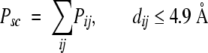
Side-chain interaction preference penalty (P_sc)

The amino acids in membrane proteins show a preference for which amino acids they interact with on neighboring helices (Adamian and Liang 2001; Nikiforovich et al. 2001; Adamian et al. 2003). To evaluate this characteristic in our candidate helical bundles, we incorporate the membrane helical interfacial pairwise (MHIP) amino acid interaction propensity matrix of Adamian and Liang (Adamian and Liang 2001) into our penalty function. The entries of this matrix have been adjusted to reflect penalties for low propensity pair interactions rather than bonuses for favored pair interactions by subtracting the propensity score for each amino acid pair from the value of the highest propensity pair (Table 4). Note that the penalty for the strongest interacting pairs, such as CYS–GLN, which have an MHIP = 6.0, is now 0.0, while the penalty on the weakest interacting pairs, such as ARG–SER with an MHIP = 0.0, is now 6.0, the largest value in Table 4. The side-chain propensity penalty is simply the sum of the pairwise propensity over all side-chain pairs, for which the Cβ atoms are within 4.9 Å of each other,

Table 4.

Helical interfacial side-chain packing penalties

	ALA	CYS	ASP	GLU	PHE	GLY	HIS	ILE	LYS	LEU	MET	ASN	PRO	GLN	ARG	SER	THR	Val	TRP	TYR
ALA	4.7	4.3	4.8	5.2	4.9	4.9	4.7	5.0	5.3	5.1	4.3	4.9	3.9	5.0	5.5	5.1	5.0	5.2	4.9	5.2
CYS	4.3	5.2	6.0	5.2	4.2	3.6	4.7	4.9	6.0	5.0	4.5	5.2	5.4	6.0	5.6	3.8	4.8	5.7	5.6	5.7
ASP	4.8	6.0	6.0	5.6	5.7	5.9	5.4	5.0	3.8	5.3	5.5	1.2	4.2	6.0	2.3	4.8	5.0	5.9	5.6	3.2
GLU	5.2	5.2	5.6	4.4	5.5	5.3	5.0	5.6	4.3	5.5	5.0	4.7	4.1	5.6	4.8	5.0	5.0	5.3	5.9	5.3
PHE	4.9	4.2	5.7	5.5	4.3	4.7	4.9	5.2	5.6	4.9	4.6	5.5	5.4	5.0	5.6	5.0	5.3	5.1	4.6	5.2
GLY	4.9	3.6	5.9	5.3	4.7	3.0	2.9	5.4	5.6	5.0	4.7	4.4	5.4	4.6	5.4	5.0	5.4	5.0	4.6	4.4
HIS	4.7	4.7	5.4	5.0	4.9	2.9	2.1	5.3	5.5	5.3	5.0	5.8	5.7	3.5	5.7	4.7	3.7	5.5	4.1	4.8
ILE	5.0	4.9	5.0	5.6	5.2	5.4	5.3	4.7	5.5	5.0	4.9	4.9	4.8	5.0	5.8	5.4	5.1	5.2	5.0	5.5
LYS	5.3	6.0	3.8	4.3	5.6	5.6	5.5	5.5	6.0	5.3	3.8	3.2	5.0	4.4	5.2	4.9	5.8	5.6	5.4	3.5
LEU	5.1	5.0	5.3	5.5	4.9	5.0	5.3	5.0	5.3	4.9	5.0	5.1	5.3	5.2	5.4	4.9	5.4	5.0	5.0	5.0
MET	4.3	4.5	5.5	5.0	4.6	4.7	5.0	4.9	3.8	5.0	4.5	5.2	4.6	5.0	4.7	4.1	5.3	5.1	4.8	5.4
ASN	4.9	5.2	1.2	4.7	5.5	4.4	5.8	4.9	3.2	5.1	5.2	0.0	4.8	3.6	5.3	4.6	5.2	5.1	5.3	4.5
PRO	3.9	5.4	4.2	4.1	5.4	5.4	5.7	4.8	5.0	5.3	4.6	4.8	4.2	5.1	5.4	4.8	4.7	5.4	4.8	4.0
GLN	5.0	6.0	6.0	5.6	5.0	4.6	3.5	5.0	4.4	5.2	5.0	3.6	5.1	6.0	3.2	3.5	4.6	5.3	4.7	3.7
ARG	5.5	5.6	2.3	4.8	5.6	5.4	5.7	5.8	5.2	5.4	4.7	5.3	5.4	3.2	6.0	0.0	5.0	5.0	1.0	5.0
SER	5.1	3.8	4.8	5.0	5.0	5.0	4.7	5.4	4.9	4.9	4.1	4.6	4.8	3.5	0.0	1.6	4.5	5.2	4.9	5.0
THR	5.0	4.8	5.0	5.0	5.3	5.4	3.7	5.1	5.8	5.4	5.3	5.2	4.7	4.6	5.0	4.5	4.9	4.9	4.9	4.8
VAL	5.2	5.7	5.9	5.3	5.1	5.0	5.5	5.2	5.6	5.0	5.1	5.1	5.4	5.3	5.0	5.2	4.9	5.0	5.1	5.5
TRP	4.9	5.6	5.6	5.9	4.6	4.6	4.1	5.0	5.4	5.0	4.8	5.3	4.8	4.7	1.0	4.9	4.9	5.1	5.2	5.1
TYR	5.2	5.7	3.2	5.3	5.2	4.4	4.8	5.5	3.5	5.0	5.4	4.5	4.0	3.7	5.0	5.0	4.8	5.1	5.1	5.4

Penalties are the membrane helical interfacial pairwise contact propensities from Adamian and Liang (2001) for which each propensity has been subtracted from the highest propensity to yield a penalty for preferred side chains not interacting.

(10)

where P_ij is the interaction penalty of amino acids i and j, and d_ij is the distance between the two Cβ atoms.

Total score

The total score is the sum of the individual components, which are summed over the appropriate set of pairwise interactions. Let m be the number of helices, n the number of amino acids, Ω the set of amino acids among which distances have been measured, Γ the set of m(m − 1)/2 distinct helical pairs, and Λ the set of n(n − 1)/2 distinct Cβ pairs. Then, the Bundler penalty can be written as:

(11)

Scoring function validation

Given the small sample size of transmembrane helical bundles from which to draw a picture of the “average” transmembrane helical bundle, we did not necessarily expect Bundler to identify the native structure as the least penalized bundle. Rather, we expected to be able to coarsely group bundles in such a way that their penalty would identify how near or far a given model bundle is from the native bundle, and that these groupings would be dependent on the class of membrane protein from which a helical bundle is a member. This is a reasonable expectation when one considers that the minimum score structure represents the average bundle across a diverse set of transmembrane helices. As a result, we placed only modest demands on the Bundler penalty function. Our principal requirement is that it can be calibrated in such a way that the score of near-native structures clearly differentiates them from structures that are not likely to be native bundles.

To determine whether or not Bundler is capable of distinguishing the known helical bundle from a set of helical bundles close to the PDB structure, we analyzed the helical bundles of six known membrane proteins. Helical bundles were extracted as is (i.e., any distortions from ideality were maintained) from the PDB files, and only those portions of the transmembrane helices completely embedded in the membrane were considered. For example, the two short helices, 76–86 and 192–202, of Aquaporin (1fqy.pdb) only partially insert into the membrane and thus were excluded. For each structure, we derived a set of Cα to Cα distances corresponding to pairs of amino acids (K–K, K–D, K–E, K–C, and C–C) that could potentially be obtained via chemical cross-linking using commercially available chemical cross-linkers and then added a 4 Å error to each distance. Five hundred bundles were generated for each test case by running a Monte Carlo simulated annealing algorithm at 500 K, a temperature high enough to generate a set of structures with an RMSD spectrum of several angstroms. Specifically, we considered the following six helical bundles (PDB identifier, number of helices and number of distance constraints, respectively, are given in parentheses): bacteriorhodopsin (1c3w, 7, 60), halorhodopsin (1e12, 7, 9), rhodopsin (1f88, 7, 38), aquaporin-1 (1fqy, 6, 17), sensory rhodopsin (1jgj, 7, 18), and a subunit of fumarate reductase flavoprotein (1qlaC, 5, 58).

Figure 2 ▶ displays the results for all six test cases as plots of the Bundler function value versus distance from the known structure measured using the RMSD across the Cα atoms (Cα–RMSD). The scatter plots show the results for a representative case of 500 structures generated as outlined above for each of the test proteins. In all cases, the helical bundle from the PDB file has the lowest Bundler penalty. Moreover, the general trend is that bundles closer in Cα–RMSD to the known structure have lower Bundler penalty scores than those farther from the known structure. In the case of aquaporin, while the known structure had the lowest penalty, the correlation between distance from the known structure and penalty was not as strong. This lack of correlation for aquaporin may be due to the fact that we are including only the transmembrane helices that span the membrane and omitting two short helices that are only partially inserted into the membrane, which most impacts the contacts penalty portion of the Bundler score: Omission of the two short helices removes neighbors within the cutoff distance from several helices that increases the contacts penalty.

Figure 2.

Bundler penalty as a function of RMSD from the X-ray structure for six integral membrane proteins. Sets of 500 structures were generated using a Monte Carlo simulated annealing algorithm at a single high temperature as described in the text. Scatter plots show the results for a typical single set of 500 structures. Bar charts show the mean and standard error of 10 sets of 500 structures each generated with different random number streams. The number of helices and the number of distances are provided in the inset of each scatter plot.

To further test the robustness of Bundler at predicting native like helical bundles, we generated 10 sets, using different random number streams, of 500 structures for each of the six test proteins. These structures were then grouped into 2 Å bins and the mean and standard deviation of the penalty was calculated within each bin (Fig. 2 ▶). Overall, the structures with lower Bundler scores correspond to structures closer to the target or native structure. Thus, it is reasonable to expect that the models with the lowest Bundler scores represent structures within a few Angstroms of their corresponding native bundle. The variation in penalty within each group is small, suggesting that the trend is not due to the presence of a few very low penalty structures and a few very high penalty structures. We can thus be confident that a bundle with a higher Bundler score is not close to the native-like bundle and the bundles with the lowest Bundler penalty represent the most native-like bundles among the set of possible models. Excluding aquaporin, these results also provide sufficient evidence that an upper bound on the Bundler penalty can be set and used to pick a subset of models for further refinement. For example, model bundles with a Bundler penalty of less than 2000, or more conservatively 3000, are good candidates for further refinement by penalty function minimization.

Two-step approach to modeling transmembrane helical bundles using sparse distance constraints to build the rhodopsin helical bundle

The overall goal of this work was to develop a technique for building the transmembrane helical bundles of integral membrane proteins given a sparse set of distance constraints. In this section, we demonstrate a two-step approach to modeling transmembrane helical bundles. This method combines our previous work on searching the conformational space of membrane protein bundles satisfying a set of distance constraints (Faulon et al. 2003) with Monte Carlo simulated annealing (MCSA) of the empirical scoring function described in the previous sections. The method is designed to provide a computationally efficient means of searching the conformational space of the helical bundle by first searching the global space of all possible helical bundles to find those satisfying a given set of distance constraints and then searching the local conformational space of each of these candidate models. Each step is detailed in the Materials and Methods section.

The method is demonstrated using the seven transmembrane helices from the rhodopsin crystal structure 1f88.pdb, and a set of 27 distances constraints compiled from various experiments, reported in the literature, and summarized by Yeagle et al. (2001). These included dipolar EPR distances (Farrens et al. 1996; Yang et al. 1996; Albert et al. 1997; Galasco et al. 2000), disulfide mapping distances (Yu et al. 1995, 1999; Sheikh et al. 1996; Cai et al. 1997, 1999) and distances from electron cryomicroscopy (Unger and Schertler 1995; Yeagle et al. 2001). These distance constraints are given in Table 5 and have an average error of ±3.75 Å.

Table 5.

Experimental distances used for modeling the rhodopsin helical bundle

Helix1	Helix2	Residue1	Residue2	Minimum distance	Maximum distance	Experimental method	Reference
C	F	139	248	6	20	Dipolar SDSL-EPRa	Farrens et al. 1996
C	F	139	249	9	26	Dipolar SDSL-EPRa	Farrens et al. 1996
C	F	139	250	9	26	Dipolar SDSL-EPRa	Farrens et al. 1996
C	F	139	251	6	20	Dipolar SDSL-EPRa	Farrens et al. 1996
C	F	139	252	9	26	Dipolar SDSL-EPRa	Farrens et al. 1996
A	G	65	316	4	19	Dipolar SDSL-EPRa	Yang et al. 1996
E	F	204	276	4	8	Disulfide mappingb	Yu et al. 1995
C	E	140	222	4	8	Disulfide mappingb	Yu et al. 1999
C	E	140	225	4	8	Disulfide mappingb	Yu et al. 1999
C	F	135	250	4	8	Disulfide mappingb	Yu et al. 1999
C	E	136	222	4	8	Disulfide mappingb	Cai et al. 1997
C	E	136	225	4	8	Disulfide mappingb	Cai et al. 1997
B	C	71	134	9	13	Electron diffractionc	Unger and Schertler 1995; Yeagle et al. 2001
B	C	90	116	5	10	Electron diffractionc	Unger and Schertler 1995; Yeagle et al. 2001
B	D	71	153	5	10	Electron diffractionc	Unger and Schertler 1995; Yeagle et al. 2001
B	D	86	172	15	20	Electron diffractionc	Unger and Schertler 1995; Yeagle et al. 2001
C	E	136	226	6	9	Electron diffractionc	Unger and Schertler 1995; Yeagle et al. 2001
C	E	125	215	6	9	Electron diffractionc	Unger and Schertler 1995; Yeagle et al. 2001
D	E	152	225	18	22	Electron diffractionc	Unger and Schertler 1995; Yeagle et al. 2001
E	F	216	258	9	13	Electron diffractionc	Unger and Schertler 1995; Yeagle et al. 2001
F	G	253	305	6	8	Electron diffractionc	Unger and Schertler 1995; Yeagle et al. 2001
F	G	264	298	6	8	Electron diffractionc	Unger and Schertler 1995; Yeagle et al. 2001
A	G	39	286	9	14	Electron diffractionc	Unger and Schertler 1995; Yeagle et al. 2001
C	F	114	268	14	18	Electron diffractionc	Unger and Schertler 1995; Yeagle et al. 2001
D	F	171	268	17	20	Electron diffractionc	Unger and Schertler 1995; Yeagle et al. 2001
B	F	73	250	10	15	Electron diffractionc	Unger and Schertler 1995; Yeagle et al. 2001
A	F	62	250	16	20	Electron diffractionc	Unger and Schertler 1995; Yeagle et al. 2001
A	F	47	264	16	19	Electron diffractionc	Unger and Schertler 1995; Yeagle et al. 2001

Helices A, B, C, D, E, F, G correspond to residues 33–65, 70–101, 105–140, 149–173, 199–226, 245–278, and 284–309, respectively.

^a Reported distance ranges were adjusted to account for the error involved in using spin–spin distances as Cα–Cα distances as described in the text.

^b Cα–Cα distances from disulfide mapping were set to 5.68 Å ± (reported error) as described in the text.

^c Cα–Cα distances correspond to distances measured from the top, middle, and bottom of consecutive helices as described by Yeagle et al. (2001).

Because the published EPR dipolar distances are between nitroxide spin labels, they do not directly correspond to distances between helical axes. To better represent these distances, we determined the error associated with interpreting spin–spin distances as Cα–Cα distances by comparing the two measures in proteins for which distances have been measured by EPR and a crystal structure is also available. We used a total of 16 measures for this analysis including six from rhodopsin (1F88; Farrens et al. 1996^; Yang et al. 1996^; Palcewski et al. 2000), four from human carbonic anhydrase II (Hakansson et al. 1992; Persson et al. 2001), four from T4-lysozyme (3LZM; Matsumura et al. 1989^; McHaourab et al. 1997), and one each from maltose-binding protein liganded form (1MDP; Sharff et al. 1995^; Hall et al. 1997) and maltose-binding protein unliganded form (1DMB; Sharff et al. 1993). From this analysis, we determined the difference between spin–spin distances and Cα–Cα distances to be 4.3 ± 1.8 Å. We used this distance to adjust the lower and upper limits of the reported distances to better represent the internitroxide distances as helix backbone distances. We use the reported distance plus 6 Å as an upper bound and either the minimum of the reported distance minus 6 Å and 4 Å as a lower bound. For the disulfide mapping distances, we use a Cα to Cα distance of 5.68 Å, which corresponds to two Cβ to Sγ bonds (1.82 Å) and one Sγ to Sγ bond (2.04 Å), plus or minus the reported error.

In a recent article (Faulon et al. 2003), we described a method for searching the conformation space of a set of transmembrane helices for bundles matching a given set of distance constraints. Applying this method to the seven rhodopsin helices using the 27 distance constraints given in Table 5 reduced the approximately 7.0 × 10¹¹ possible seven-helix configurations to only 87 helical bundles with Cα –RMSDs ranging from 4.3 Å to 9.5 Å (Faulon et al. 2003). Thus, given only 27 distance constraints from a variety of experimental methods with differing levels of error, we were able to extract a reasonable number of structures suitable for further refinement from an overwhelmingly large data set of possible helix bundles.

We refined each of these 87 structures using the Monte Carlo simulated annealing (MCSA) protocol described in the Materials and Methods section. The local conformation space of each helical bundle was searched for the structure with the minimum Bundler penalty function value. Because our goal is only to search the local conformational space of each bundle in a way that allows uphill moves over small barriers within a larger penalty function minima, we use a starting temperature of 30 and a geometric cooling schedule with the cooling constant set at 0.9 (i.e, T_i = 0.9T_i−1). A temperature cycle was terminated after either a total of 1000 structures were generated or after 100 structures were accepted, whichever occurred first. The MCSA simulations were run for 34 temperature steps.

The least penalized structure in this cluster has a penalty of 3.3 and a Cα–RMSD from the known structure of 4.1 Å. Compared to the scores of the decoy structures tabulated in Figure 2 ▶, the Bundler penalty on this structure is much lower than those of the lowest RMSD helix assemblies. This indicates that models with Bundler penalties in the range of 1000 to 2000 should have properties most similar to those of an “average” membrane protein helical bundle, while satisfying a set of experimental distance constraints. Among the 87 refined bundles, several have minimized penalties around 1000. The least penalized bundle among these has a Bundler score of 1003.3 and a Cα–RMSD of 3.2 Å (Fig. 3 ▶). This result again provides evidence that simply minimizing an empirical structure-based penalty function may not produce the ultimate best structure. Minimization drives the structure toward an “average” structure, which is not the most native-like structure for a particular protein. It is therefore essential to calibrate the function to a particular family of structures. Our results show that for seven helix bundles, the most native-like structures have Bundler penalties between approximately 1000 and 2000, which provides a better stopping criterion for our MCSA refinement protocol. For example, we could anneal the structure using a faster cooling schedule, until reaching a penalty of 2000 and then slow the cooling to more thoroughly sample conformations with Bundler scores between 1000 and 2000. The search will ultimately be stopped when the Bundler penalty drops below 1000.

Figure 3.

Comparison of the predicted helical bundle (black) to the X-ray structure (1F88.pdb) helical bundle (gray). The Cα–RMSD between the two structures is 3.2 Å. As is clearly visible the helices are correctly arranged, and most of the deviation is due to differences in helical tilt angles.

Discussion

Due to the difficulties of using the standard structure determination methods for structural modeling of transmembrane proteins, it is important to develop methods using more easily obtainable, but lower resolution, data. With this in mind, we have developed a method for using sparse distance constraints to model the transmembrane spanning domain. Development of such a method is particularly timely and important given the progress in using methods such as chemical cross-linking, dipolar EPR, and FRET for providing distance constraints.

We have presented a two-step approach to modeling transmembrane helical bundles and demonstrated its effectiveness by accurately modeling the transmembrane helical bundle of dark-adapted rhodopsin. In the first step, the set of all possible helical bundles is generated and filtered to find the set of bundles that satisfy the set of distance constraints using a previously reported algorithm (Faulon et al. 2003). In Step 2, the structures from Step 1 are refined using a Monte Carlo simulated annealing protocol to minimize a scoring function that penalizes helical arrangements that violate distance constraints and that violate constraints derived from a statistical analysis of solved membrane protein structures from the PDB. Using a set of 27 experimental distance constraints extracted from the literature, we modeled the helical bundle of dark-adapted bovine rhodopsin to within 3.2 Å of the X-ray structure.

A major component of this work was the development and validation of a penalty function designed to discriminate near-native helical bundles from those far from the native structure and thus build transmembrane helical bundles that are consistent with both experimental distance constraints and other helical bundles from known structures. Because the majority of known transmembrane protein structures are seven helix bundles, it is not surprising that the Bundler penalty function works very well for this class of membrane proteins (Fig. 2 ▶). However, we have also illustrated that Bundler can be useful for modeling other classes of helical bundles (e.g., aquaporin, fumarate reductase flavoprotein).

In the case of aquaporin, the correlation between the RMSD from the crystal structure and the Bundler score is less pronounced than for the other validation cases. Inspection of Bundler’s components revealed that the relatively higher scores are due to larger contacts penalties resulting from a reduction in the number of neighboring helices within the cutoff distance, presumably caused by removal of the two partially inserted helices. Moreover, there is a high side-chain interaction preference penalty and a high helix packing angle penalty for some of the lower RMSD bundles. This again is likely due to the removal of the partially inserted helices, which in this case is likely to have removed favorable side-chain interactions and reduced the overall helix packing, allowing nontypical helix tilt angles.

Clearly, a structure-based penalty function for helical membrane bundles is a work in progress that will continually be updated as more structures become available. In addition to refinements of the penalty as the database of solved membrane protein structures grows, we are also investigating the value of increasing the level of molecular detail by either representing each side-chain atom explicitly or using a reduced side-chain representation such as that described by Herzyk and Hubbard (1993). Additionally, the penalty function force constants are based on the assumption that the variance of a component scales with its importance as a predictor and as such are somewhat arbitrary. Refinement of these parameters against, for example, our databases of decoy structures may also improve the penalty function. We are also exploring ways to include, either explicitly or implicitly, ligands such as retinal. Increased structural detail will impact the packing parameters of the helical bundle by enhancing the level of detail of side-chain van der Waals interactions and by increasing the accuracy of packing density calculations. The inclusion of ligands such as retinal may be necessary to more accurately predict helix–helix interactions that are unlike those of an average bundle. For example, in helix bundles containing a ligand, additional van der Waals interactions between helix atoms and the ligand may be necessary to force the associated helices of the bundle outside the range of allowed distances or angles derived from idealized versions of solved structures without ligands.

Moreover, our results in using this method to recover the structure of rhodopsin prompt questions as to whether similar results could be obtained using fewer distances and how the accuracy of a helical bundle generally varies with number of distance. In response, we note that the determination of accuracy solely as a function of the number of distances is nontrivial. Previously, we showed that the number of possible helical bundles simultaneously satisfying a set of distance constraints varies with the number of distances, the error on these distances, and the radius of the associated distance graph or, in other words, the way in which the distances are distributed among and connect the helices (Faulon et al. 2003). This result likely carries over to the accuracy of modeling membrane proteins using Bundler; however, we have not yet carried out the extensive analysis required to confirm this assumption. For now, it suffices to say that only a modest number of distances are needed to build accurate models of transmembrane helical bundles using the approach outlined here.

It remains to be seen whether or not a truly general function useful for refining helix bundles with a range of secondary structural elements can be developed. Although it is likely that the form of the penalty function presented in this article utilizes many necessary structural components, the determination of a broader range of structures with a varying number of transmembrane secondary structural elements may result in separate sets of statistical parameters that depend on the number of these elements. Regardless of such future findings, the approach proposed here is general, and Bundler is easily adaptable to new statistics based parameterization.

Materials and methods

Representation of the helical bundle

For the test cases used in this study, the helices were obtained using the helix definitions provided in the PDB file. All side chain atoms beyond the Cβ were removed (i.e., we represent the helix in its native form at the Cβ level of detail). Helices are treated as rigid bodies with the helical axis defined as the line segment between the unweighted centers of mass of the last four residues of the C and N termini.

Assembly of membrane protein data set

The membrane proteins used in this work were selected from the list of solved structures generously provided by Professor Stephen H. White at the University of California, Irvine (http://blanco.biomol.uci.edu/Membrane_Proteins_xtal.html). Proteins without definable backbone atom positions were not used (e.g., 2PPS, 1FE1). Monomers, if they form a compact folding unit, were used. An exception was made for small monomers that pack together to form a helical bundle; in those cases, the entire bundle was used (e.g., 1BL8). If the structure of a single protein was solved more than once, we selected the structure of the highest resolution, and if the structure was solved for multiple species, the structure for the species with the highest resolution was chosen. Heteromultimeric complexes were parsed to remove all but the transmembrane bundle subunits (e.g., 1EZVC). Helices that only partially span the membrane were removed from the final bundle structures (e.g., 1FQY).

Determination of force constants

The variance in the measured properties of transmembrane protein bundles is a good indicator of the importance of a given property in predicting the fold of a helical bundle. We use the variance from our analysis of a set of nonredundant structures to guide our choices of force constants in the Bundler penalty function. Those measures having the smallest variances as a percentage of the mean were assumed to be better descriptors of a helical bundle, and were assigned a force constant of 500. The largest variance measure, the packing angle, is assigned a force constant of 5, and the remaining force constants were given intermediate values.

We have recently shown the importance of distance constraints in exploring the conformational space of helical bundles and in reducing the number of candidate structures for local conformational search to a reasonable number (Faulon et al. 2003). To accurately represent this importance in Bundler, we set the force constant for experimental distance constraints to the highest value of 500.

Conformational search under a set of distance constraints

Details of our procedure for exploring the conformational space of membrane protein folds matching distance constraints are provided in Faulon et al. 2003 and are summarized in the methods section. Briefly, the procedure generates an exhaustive set of helix bundles within a specified RMSD by positioning the helices such that distance constraints are satisfied. The data required by Step 1 are a set of individual helices in PDB format that we assume has been modeled and optimized and a set of distances. Step 1 results in a set of all possible helical bundles matching the distances such that the bundles in the set differ from one another by some user defined RMSD. These helical arrangements are described at an atomistic level suitable for further refinement by local conformational search (Step 2).

Monte Carlo simulated annealing

In Step 2 of our procedure for building an optimized helical bundle, we refine a subset of the structures from the conformational search Step 1 using the Bundler penalty function developed in this article and a Monte Carlo simulated annealing (MCSA) protocol to search the local conformational space of the bundle.

Helical bundle

A helical bundle is defined as any arrangement of the helices in Cartesian coordinate space. The helix z-axis (z′ in Fig. 4 ▶) is defined as the line segment connecting the average coordinates of the N and C termini for each helix (Fig. 4 ▶). Each helix has six degrees of freedom, consisting of translations in the global (x, y, z) axis system and rotations in the (x′, y′, z′) axis system (Fig. 4 ▶), giving a systemwide total of 6n degrees of freedom, where n is the number of helices.

Figure 4.

Definition of helix axis system (left) and helix degrees of freedom (right). The helix z-axis is defined as the vector connecting the average coordinates of the last four residues of the helix N and C termini. Helix degrees of freedom include translations in the global (x, y, z) axis system and x′, y′, and z′ rotations around the helix axes.

Monte Carlo sampling

Starting from the last accepted arrangement, a new helical bundle is generated by randomly selecting one of the secondary structural elements (SSEs) and randomizing its position by either translation in the global axis system (x, y, z) or rotation in the local axis system (x′, y′, z′) (Fig. 4 ▶). Similar to those used by Herzyk and Hubbard (1995), four moves are possible (Fig. 4 ▶): (1) translation along the z, (2) two consecutive translations along the x and y, (3) rotation around z′, or (4) two consecutive rotations around x′and y′. The size of this move is chosen randomly within some user defined limits. If the Bundler penalty of the new structure is lower than that of the current lowest scoring structure, then that structure is accepted as the current structure. Otherwise, the Boltzmann probability factor, p, is calculated as e^−ΔP/T, where ΔP is the difference in total penalty between the least penalized structure and the newly generated structure and T is the temperature, which in this case is simply a parameter for controlling the probability of a given helical bundle (Kirkpatrick et al. 1983). Then p is compared to a random number, r, from a uniform [0,1] distribution. If p < r, the new configuration is accepted as the new best structure; otherwise, the new bundle is rejected (Metropolis et al. 1958).

Cooling schedule

The cooling schedule used for the refinements of Step 2 started at T = 30, and was reduced at each new temperature cycle according to a geometric temperature schedule with the temperature reduction factor set to 0.95 (i.e., T_i = 0.95T_i−1). Thirty-four temperature cycles were completed, and each temperature cycle terminated after either 1000 Monte Carlo steps were completed or after 100 candidate structures were accepted.

Structural analysis and data processing

Membrane protein statistics were calculated using in-house software. RMSD calculations and various manipulations of PDB files were performed using the Multiscale Modeling Tools in Structural Biology (MMTSB) toolset (Feig et al. 2001). Molecular visualization and renderings were obtained using VMD (Humphrey et al. 1996). All analysis of the penalty data was done using programs written in MATLAB 6.5 (The Math Works Inc.).

Article published online ahead of print. Article and publication date are at http://www.proteinscience.org/cgi/doi/10.1110/ps.04781504.

References

- Adamian, L. and Liang, J. 2001. Helix–helix packing and interfacial pairwise interactions of residues in membrane proteins. J. Mol. Biol. 311 891–907. [DOI] [PubMed] [Google Scholar]
- Adamian, L., Jackups Jr., R., Binkowski, T.A., and Liang, J. 2003. Higher-order interhelical spatial interactions in membrane proteins. J. Mol. Biol. 327 251–272. [DOI] [PubMed] [Google Scholar]
- Albert, A.D., Watts, A., Spooner, P., Grobner, G., Young, J., and Yeagle, P.L. 1997. A solid state NMR characterization of the substrate binding specificity and dynamics for the L-fucose-H+ membrane transport protein of E. coli. Biochim. Biophys. Acta 1328 74–82. [DOI] [PubMed] [Google Scholar]
- Altenbach, C., Oh, K.J., Trabanino, R.J., Hideg, K., and Hubbell, W.L. 2001. Estimation of inter-residue distances in spin labeled proteins at physiological temperatures: Experimental strategies and practical limitations. Biochemistry 40 15471–15482. [DOI] [PubMed] [Google Scholar]
- Back, J.W., Sanz, M.A., De Jong, L., De Koning, L.J., Nijtmans, L.G., De Koster, C.G., Grivell, L.A., Van Der Spek, H., and Muijsers, A.O. 2002. A structure for the yeast prohibitin complex: Structure prediction and evidence from chemical crosslinking and mass spectrometry. Protein Sci. 11 2471–2478. [DOI] [PMC free article] [PubMed] [Google Scholar]
- Bennett, K.L., Kussmann, M., Bjork, P., Godzwon, M., Mikkelsen, M., Sorensen, P., and Roepstorff, P. 2000. Chemical cross-linking with thiolcleavable reagents combined with differential mass spectrometric peptide mapping—A novel approach to assess intermolecular protein contacts. Protein Sci. 9 1503–1518. [DOI] [PMC free article] [PubMed] [Google Scholar]
- Borbat, P.P., Costa-Filho, A.J., Earle, K.A., Moscicki, J.K., and Freed, J.H. 2001. Electron spin resonance in studies of membranes and proteins. Science 291 266–269. [DOI] [PubMed] [Google Scholar]
- Bowie, J.U. 1997. Helix packing in membrane proteins. J. Mol. Biol. 272 780–789. [DOI] [PubMed] [Google Scholar]
- ———. 1999. Helix-bundle membrane protein fold templates. Protein Sci. 8 2711–2719. [DOI] [PMC free article] [PubMed] [Google Scholar]
- Brown, L.J., Sale, K.L., Hills, R., Rouviere, C., Song, L., Zhang, X., and Fajer, P.G. 2002. Structure of the inhibitory region of troponin by site directed spin labeling electron paramagnetic resonance. Proc. Natl. Acad. Sci. 99 12765–12770. [DOI] [PMC free article] [PubMed] [Google Scholar]
- Brünger, A.T., Adams, P.D., Clore, G.M., DeLano, W.L., Gros, P., Grosse-Kunstleve, R.W., Jiang, J.S., Kuszewski, J., Nilges, M., Pannu, N.S., et al. 1998. Crystallography & NMR system: A new software suite for macro-molecular structure determination. Acta Crystallogr. D 54 905–921. [DOI] [PubMed] [Google Scholar]
- Buchan, D., Shephard, D., Lee, D., Peral, F., Rison, S., Thorton, J., and Orengo, C. 2002. Structural assignment for whole genes and genomes using the CATH domain structure database. Genome Res. 12 503–514. [DOI] [PMC free article] [PubMed] [Google Scholar]
- Cai, K., Langen, R., Hubbell, W.L., and Khorana, H.G. 1997. Structure and function in rhodopsin: Topology of the C-terminal polypeptide chain in relation to the cytoplasmic loops. Proc. Natl. Acad. Sci. 94 14267–14272. [DOI] [PMC free article] [PubMed] [Google Scholar]
- Cai, K., Klein-Seetharaman, J., Hwa, J., Hubbell, W.L., and Khorana, H.G. 1999. Structure and function in rhodopsin. Effects of disulfide cross-links in the cytoplasmic face of rhodopsin on transducin activation and phosphorylation by rhodopsin kinase. Biochemistry 38 12893–12898. [DOI] [PubMed] [Google Scholar]
- Cai, K., Klein-Seetharaman, J., Altenbach, C., Hubbell, W.L., and Khorana, H.G. 2001. Probing the dark state tertiary structure in the cytoplasmic domain of rhodopsin: Proximities between amino acids deduced from spontaneous disulfide bond formation between cysteine pairs engineered in cytoplasmic loops 1, 3, and 4. Biochemistry 40 12479–12485. [DOI] [PubMed] [Google Scholar]
- Chothia, C. 1975. Structural invariants in protein folding. Nature 254 304–308. [DOI] [PubMed] [Google Scholar]
- Dihazi, G.H., and Sinz, A. 2003. Mapping low-resolution three-dimensional protein structures using chemical cross-linking and Fourier transform ion-cyclotron resonance mass spectrometry. Rapid Commun. Mass Spectrom. 17 2005–2014. [DOI] [PubMed] [Google Scholar]
- Dobbs, H., Orlandini, E., Bonaccini, R., and Seno, F. 2002. Optimal potentials for predicting inter-helical packing in transmembrane proteins. Proteins 49 342–349. [DOI] [PubMed] [Google Scholar]
- Engelman, D.M., Steitz, T.A., and Goldman, A. 1986. Identifying nonpolar transbilayer helices in amino acid sequences of membrane proteins. Annu. Rev. Biophys. Biophys. Chem. 15 321–353. [DOI] [PubMed] [Google Scholar]
- Farrens, D.L., Altenbach, C., Yang, K., Hubbell, W.L., and Khorana, H.G. 1996. Requirement of rigid-body motion of transmembrane helices for light activation of rhodopsin. Science 274 768–770. [DOI] [PubMed] [Google Scholar]
- Faulon, J.-L., Sale, K., and Young, M. 2003. Exploring the conformational space of membrane protein folds matching distance constraints. Protein Sci. 12 1750–1761. [DOI] [PMC free article] [PubMed] [Google Scholar]
- Feig, M., Karanicolas, J., and Brooks, C.L.I. 2001. MMTSB tool set. MMTSB NIH Research Resource, The Scripps Research Institute, La Jolla, CA.
- Fleishman, S.J. and Ben-Tal, N. 2002. A novel scoring function for predicting the conformations of tightly packed pairs of transmembrane α-helices. J. Mol. Biol. 321 363–378. [DOI] [PubMed] [Google Scholar]
- Galasco, A., Crouch, R.K., and Knapp, D.R. 2000. Intrahelic arrangement in the integral membrane protein rhodopsin investigated by site-specific chemical cleavage and mass spectrometry. Biochemistry 39 4907–4914. [DOI] [PubMed] [Google Scholar]
- Hakansson, K., Carlsson, M., Svensson, L.A., and Liljas, A. 1992. Structure of native and apo carbonic anhydrase II and structure of some of its anion-ligand complexes. J. Mol. Biol. 227 1192–1204. [DOI] [PubMed] [Google Scholar]
- Hall, J.A., Thorgeirsson, T.E., Liu, J., Shin, Y.K., and Nikaido, H. 1997. Two modes of ligand binding in maltose-binding protein of Escherichia coli. Electron paramagnetic resonance study of ligand-induced global conformational changes by site-directed spin labeling. J. Biol. Chem. 272 17610–17614. [DOI] [PubMed] [Google Scholar]
- Herzyk, P., and Hubbard, R.E. 1993. A reduced representation of proteins for use in restraint satisfaction calculations. Proteins 17 310–324. [DOI] [PubMed] [Google Scholar]
- ———. 1995. Automated method for modeling seven-helix transmembrane receptors from experimental data. Biophys. J. 69 2419–2442. [DOI] [PMC free article] [PubMed] [Google Scholar]
- Hillisch, A., Lorenz, M., and Diekmann, S. 2001. Recent advances in FRET: Distance determination in protein–DNA complexes. Curr. Opin. Struct. Biol. 11 201–207. [DOI] [PubMed] [Google Scholar]
- Hubbell, W.L., Altenbach, C., Hubbell, C.M., and Khorana, H.G. 2003. Rhodopsin structure, dynamics, and activation: A perspective from crystallography, site-directed spin labeling, sulfhydryl reactivity, and disulfide cross-linking. Adv. Protein Chem. 63 243–290. [DOI] [PubMed] [Google Scholar]
- Humphrey, W., Dalke, A., and Schulten, K. 1996. VMD—Visual molecular dynamics. J. Mol. Graph. 14 33–38. [DOI] [PubMed] [Google Scholar]
- Hustedt, E.J. and Beth, A.H. 1999. Nitroxide spin–spin interactions: Applications to protein structure and dynamics. Annu. Rev. Biophys. Biomol. Struct. 28 129–153. [DOI] [PubMed] [Google Scholar]
- Hustedt, E.J., Smirnov, A.I., Laub, C.F., Cobb, C.E., and Beth, A.H. 1997. Molecular distances from dipolar coupled spin-labels: The global analysis of multifrequency continuous wave electron paramagnetic resonance data. Biophys. J. 72 1861–1877. [DOI] [PMC free article] [PubMed] [Google Scholar]
- Jacobs, R.E. and White, S.H. 1989. The nature of the hydrophobic binding of small peptides at the bilayer interface: Implications for the insertion of transbilayer helices. Biochemistry 28 3421–3437. [DOI] [PubMed] [Google Scholar]
- Jayasinghe, S., Hristova, K., and White, S.H. 2001a. Energetics, stability, and prediction of transmembrane helices. J. Mol. Biol. 312 927–934. [DOI] [PubMed] [Google Scholar]
- ———. 2001b. MPtopo: A database of membrane protein topology. Protein Sci. 10 455–458. [DOI] [PMC free article] [PubMed] [Google Scholar]
- Kim, S. and Cross, T.A. 2002. Uniformity, ideality, and hydrogen bonds in transmembrane α-helices. Biophys. J. 83 2084–2095. [DOI] [PMC free article] [PubMed] [Google Scholar]
- Kim, S., Chamberlain, A.K., and Bowie, J.U. 2003. A simple method for modeling transmembrane helix oligomers. J. Mol. Biol. 329 831–840. [DOI] [PubMed] [Google Scholar]
- Kirkpatrick, S., Gerlatt, C.J., and Vecchi, M. 1983. Optimization by simulated annealing. Science 220 671–680. [DOI] [PubMed] [Google Scholar]
- Klostermeier, D. and Millar, D.P. 2001. Time-resolved fluorescence resonance energy transfer: A versatile tool for the analysis of nucleic acids. Biopolymers 61 159–179. [DOI] [PubMed] [Google Scholar]
- Kruppa, G.H., Schoeniger, J., and Young, M.M. 2003. A top down approach to protein structural studies using chemical cross-linking and Fourier transform mass spectrometry. Rapid Commun. Mass Spectrom. 17 155–162. [DOI] [PubMed] [Google Scholar]
- Liu, Y.S., Sompornpisut, P., and Perozo, E. 2001. Structure of the KcsA channel intracellular gate in the open state. Nat. Struct. Biol. 8 883–887. [DOI] [PubMed] [Google Scholar]
- Matsumura, M., Wozniak, J.A., Sun, D.P., and Matthews, B.W. 1989. Structural studies of mutants of T4 lysozyme that alter hydrophobic stabilization. J. Biol. Chem. 264 16059–16066. [PubMed] [Google Scholar]
- Matyus, L. 1992. Fluorescence resonance energy transfer measurements on cell surfaces. A spectroscopic tool for determining protein interactions. J. Photochem. Photobiol. B 12 323–337. [DOI] [PubMed] [Google Scholar]
- McHaourab, H.S., Oh, K.J., Fang, C.J., and Hubbell, W.L. 1997. Conformation of T4 lysozyme in solution. Hinge-bending motion and the substrate-induced conformational transition studied by site-directed spin labeling. Biochemistry 36 307–316. [DOI] [PubMed] [Google Scholar]
- Metropolis, N., Rosenbluth, A.W., Rosenbluth, M.N., Teller, A.H., and Teller, E. 1958. Equations of state calculations by fast computing machines. J. Chem. Phys. 21 1087–1092. [Google Scholar]
- Nikiforovich, G.V., Galaktionov, S., Balodis, J., and Marshall, G.R. 2001. Novel approach to computer modeling of seven-helical transmembrane proteins: Current progress in the test case of bacteriorhodopsin. Acta Biochim. Pol. 48 53–64. [PubMed] [Google Scholar]
- Novak, P., Young, M. M., Schoeniger, J., and Kruppa, G.H. 2003. A top down approach to protein structure studies using chemical crosslinking and fourier transform mass spectrometry. Eur. J. Mass Spectrom. 9 623–631. [DOI] [PubMed] [Google Scholar]
- Palcewski, K., Kumasaka, T., Hori, T., Behnke, C.A., Motoshima, H., Fox, B.A., Le Trong, I., Teller, D.C., Okada, T., Stenkamp, R.E., et al. 2000. Crystal structure of rhodopsin: A G protein-coupled receptor. Science 289 739–745. [DOI] [PubMed] [Google Scholar]
- Parkhurst, L.J., Parkhurst, K.M., Powell, R., Wu, J., and Williams, S. 2001. Time-resolved fluorescence resonance energy transfer studies of DNA bending in double-stranded oligonucleotides and in DNA–protein complexes. Biopolymers 61 180–200. [DOI] [PubMed] [Google Scholar]
- Perozo, E., Cuello, L.G., Cortes, D.M., Liu, Y.S., and Sompornpisut, P. 2002. EPR approaches to ion channel structure and function. Novartis Found. Symp. 245 146–158; discussion 158–164, 165–168. [DOI] [PubMed] [Google Scholar]
- Persson, M., Harbridge, J.R., Hammarstrom, P., Mitri, R., Martensson, L.G., Carlsson, U., Eaton, G.R., and Eaton, S.S. 2001. Comparison of electron paramagnetic resonance methods to determine distances between spin labels on human carbonic anhydrase II. Biophys. J. 80 2886–2897. [DOI] [PMC free article] [PubMed] [Google Scholar]
- Popot, J.L. and Engelman, D.M. 1990. Membrane protein folding and oligomerization: The two-stage model. Biochemistry 29 4031–4037. [DOI] [PubMed] [Google Scholar]
- Rabenstein, M.D. and Shin, Y.K. 1995. Determination of the distance between two spin labels attached to a macromolecule. Proc. Natl. Acad. Sci. 92 8239–8243. [DOI] [PMC free article] [PubMed] [Google Scholar]
- Radzwill, N., Gerwert, K., and Steinhoff, H.J. 2001. Time-resolved detection of transient movement of helices F and G in doubly spin-labeled bacteriorhodopsin. Biophys. J. 80 2856–2866. [DOI] [PMC free article] [PubMed] [Google Scholar]
- Rappsilber, J., Siniossoglou, S., Hurt, E.C., and Mann, M. 2000. A generic strategy to analyze the spatial organization of multi-protein complexes by cross-linking and mass spectrometry. Anal. Chem. 72 267–275. [DOI] [PubMed] [Google Scholar]
- Richards, F. 1974. The interpretation of protein structures: Total volume, group volume distributions and packing density. J. Mol. Biol. 82 1–14. [DOI] [PubMed] [Google Scholar]
- Rose, G.D. 1978. Prediction of chain turns in globular proteins on a hydrophobic basis. Nature 272 586–590. [DOI] [PubMed] [Google Scholar]
- Rye, H.S. 2001. Application of fluorescence resonance energy transfer to the GroEL–GroES chaperonin reaction. Methods 24 278–288. [DOI] [PMC free article] [PubMed] [Google Scholar]
- Schilling, B., Row, R.H., Gibson, B.W., Guo, X., and Young, M.M. 2003. MS2Assign, automated assignment and nomenclature of tandem mass spectra of chemically crosslinked peptides. J. Am. Soc. Mass Spectrom. 14 834–850. [DOI] [PubMed] [Google Scholar]
- Sekar, R.B., and Periasamy, A. 2003. Fluorescence resonance energy transfer (FRET) microscopy imaging of live cell protein localizations. J. Cell Biol. 160 629–633. [DOI] [PMC free article] [PubMed] [Google Scholar]
- Sheikh, S.P., Zvyaga, T.A., Lichtarge, O., Sakmar, T.P., and Bourne, H.R. 1996. Rhodopsin activation blocked by metalion-binding sites linking transmembrane helices C and F. Nature 383 347–350. [DOI] [PubMed] [Google Scholar]
- Steinhoff, H.J., Radzwill, N., Thevis, W., Lenz, V., Brandenburg, D., Antson, A., Dodson, G., and Wollmer, A. 1997. Determination of interspin distances between spin labels attached to insulin: Comparison of electron paramagnetic resonance data with the X-ray structure. Biophys. J. 73 3287–3298. [DOI] [PMC free article] [PubMed] [Google Scholar]
- Szollosi, J., Nagy, P., Sebestyen, Z., Damjanovicha, S., Park, J.W., and Matyus, L. 2002. Applications of fluorescence resonance energy transfer for mapping biological membranes. J. Biotechnol. 82 251–266. [DOI] [PubMed] [Google Scholar]
- Taverner, T., Hall, N.E., O’Hair, R.A., and Simpson, R.J. 2002. Characterization of an antagonist interleukin-6 dimer by stable isotope labeling, cross-linking, and mass spectrometry. J. Biol. Chem. 277 46487–46492. [DOI] [PubMed] [Google Scholar]
- Unger, V.M. and Schertler, G.F. 1995. Low resolution structure of bovine rhodopsin determined by electron cryomicroscopy. Biophys. J. 68 1776–1786. [DOI] [PMC free article] [PubMed] [Google Scholar]
- Vaidehi, N., Floriano, W.B., Trabanino, R., Hall, S.E., Freddolino, P., Choi, E.J., Zamanakos, G., and Goddard III, W.A. 2002. Prediction of structure and function of G protein-couple receptors. Proc. Natl. Acad. Sci. 99 12622–12627. [DOI] [PMC free article] [PubMed] [Google Scholar]
- White, S.H. 2003. Membrane proteins of known 3D structure. http://blanco.bio-mol.uci.edu/Membrane_Proteins_xtal.html.
- White, S.H. and Wimley, W.C. 1998. Hydrophobic interactions of peptides with membrane interfaces. Biochim. Biophys. Acta 1376 339–352. [DOI] [PubMed] [Google Scholar]
- ———.1999. Membrane protein folding and stability: Physical principles. Annu. Rev. Biophys. Biomol. Struct. 28 319–365. [DOI] [PubMed] [Google Scholar]
- Wilson, S. and Bergsma, D. 2000. Orphan G-protein coupled receptors: Novel drug targets for the pharmaceutical industry. Drug Des. Discov. 17 105–114. [PubMed] [Google Scholar]
- Yang, K., Farrens, D.L., Hubbell, W.L., and Khorana, H.G. 1996. Structure and function in rhodopsin. Single cysteine substitution mutants in the cytoplasmic interhelical E-F loop region show position-specific effects in transducin activation. Biochemistry 35 14040–14046. [DOI] [PubMed] [Google Scholar]
- Yeagle, P.L., Choi, G., and Albert, A.D. 2001. Studies on the structure of the G-protein-coupled receptor rhodopsin including the putative G-protein binding site in unactivated and activated forms. Biochemistry 40 11932–11937. [DOI] [PubMed] [Google Scholar]
- Young, M., Tang, N., Hempel, J., Oshiro, C., Taylor, E., Kuntz, I., Gibson, B., and Dollinger, G. 2000. High throughput protein fold identification by using experimental constraints derived from intramolecular cross-links and mass spectrometry. Proc. Natl. Acad. Sci. 97 5802–5806. [DOI] [PMC free article] [PubMed] [Google Scholar]
- Yu, H., Kono, M., McKee, T.D., and Oprian, D.D. 1995. A general method for mapping tertiary contacts between amino acid residues in membrane embedded proteins. Biochemistry 34 14963–14969. [DOI] [PubMed] [Google Scholar]
- Yu, H., Kono, M., and Oprian, D.D. 1999. State-dependent disulfide cross-linking in rhodopsin. Biochemistry 38 12028–12032. [DOI] [PubMed] [Google Scholar]