Simulating evolution by gene duplication of protein features that require multiple amino acid residues

Abstract

Gene duplication is thought to be a major source of evolutionary innovation because it allows one copy of a gene to mutate and explore genetic space while the other copy continues to fulfill the original function. Models of the process often implicitly assume that a single mutation to the duplicated gene can confer a new selectable property. Yet some protein features, such as disulfide bonds or ligand binding sites, require the participation of two or more amino acid residues, which could require several mutations. Here we model the evolution of such protein features by what we consider to be the conceptually simplest route—point mutation in duplicated genes. We show that for very large population sizes N, where at steady state in the absence of selection the population would be expected to contain one or more duplicated alleles coding for the feature, the time to fixation in the population hovers near the inverse of the point mutation rate, and varies sluggishly with the λ^th root of 1/N, where λ is the number of nucleotide positions that must be mutated to produce the feature. At smaller population sizes, the time to fixation varies linearly with 1/N and exceeds the inverse of the point mutation rate. We conclude that, in general, to be fixed in 10⁸ generations, the production of novel protein features that require the participation of two or more amino acid residues simply by multiple point mutations in duplicated genes would entail population sizes of no less than 10⁹.

Although many scientists assume that Darwinian processes account for the evolution of complex biochemical systems, we are skeptical. Thus, rather than simply assuming the general efficacy of random mutation and selection, we want to examine, to the extent possible, which changes are reasonable to expect from a Darwinian process and which are not. We think the most tractable place to begin is with questions of protein structure. Our approach is to examine pathways that are currently considered to be likely routes of evolutionary development and see what types of changes Darwinian processes may be expected to promote along a particular pathway.

A major route of evolutionary innovation is thought to pass through gene duplication (Ohno 1970; Lynch and Conery 2000; Wagner 2001; Chothia et al. 2003). Because one copy of the gene can continue to fulfill the original function, in this view a duplicate, redundant copy of a gene is substantially free from purifying selection, allowing it to freely accumulate mutations. Although the great majority of non-neutral mutations to duplicated genes are expected to result in a null allele (Walsh 1995; Lynch and Walsh 1998), that is, a gene that no longer codes for a functional protein, occasionally one might confer a novel function on the incipient paralog. If this occurs, then the duplicated gene can be refined by mutation and positive selection, independent of the parent gene.

In most models of the development of evolutionary novelty by gene duplication, it is implicitly assumed that a single, albeit rare, mutation to the duplicated gene can confer a new selectable property (Ohta 1987; 1988a, b; Walsh 1995). However, we are particularly interested in the question of how novel protein structural features may develop throughout evolution; not all structural features of a protein may be attainable by single mutations. In particular, some protein features require the participation of multiple amino acid residues. Perhaps the simplest example of this is the disulfide bond. In order to produce a novel disulfide bond, a duplicated gene coding for a protein lacking unmatched cysteines would require at least two mutations in separate codons, and perhaps as many as six mutations, depending on the starting codons. We call protein characteristics such as disulfide bonds which require the participation of two or more amino acid residues “multiresidue” (MR) features.

A more general example of an MR feature is that of a protein binding site. A ligand bound to a protein interacts with multiple amino acid residues (Janin and Chothia 1990; Cunningham and Wells 1993; Braden and Poljak 1995; Lo et al. 1999; Chakrabarti and Janin 2002). In general, therefore, in order to produce a binding site for a new ligand in a protein originally lacking the ability to bind it, multiple mutational events would be necessary. Li (1997) drew attention to this fact in his textbook Molecular Evolution. Prefacing a discussion of the evolutionary development of the 2,3-diphosphoglycerate binding site of hemoglobin, he wrote, “acquiring a new function may require many mutational steps, and a point that needs emphasis is that the early steps might have been selectively neutral because the new function might not be manifested until a certain number of steps had already occurred” (Li 1997).

In this paper, we report the results of the stochastic simulation of the time to fixation of new MR features by what we consider to be the conceptually simplest route: point mutation in the absence of recombination in a duplicated gene that is free of purifying selection. It can be seen that, for very large populations, the expected time to fixation resides near the inverse of the mutation rate per nucleotide and decreases only slowly with the λ^th root of increasing population size, where λ is the number of nucleotide positions that must be mutated to produce the feature. For smaller populations, the time varies linearly with 1/N.

Results

The model

The model presented here assumes that newly duplicated genes encode a full-length protein with the signals necessary for its proper expression. It is further assumed that all duplicate genes are selectively neutral. (This postulate is examined in the Discussion.) Any given organism in the population may be thought to have anywhere from zero to multiple extra copies of the gene; that is, duplicate copy number is considered to have no selective effect. However, the model presupposes that there are a total of N duplicate copies of the gene, equal to the number of organisms in the population. The model assumes that either copy of a newly duplicated gene can be the one to undergo mutation and that either copy can retain the original function. That is, the original gene is not necessarily the one to retain the original function. Because the model does not include recombination, all copies of the gene accumulate point mutations independently of each other. The basic “task” that the model asks a duplicate gene to perform is to accumulate λ mutations at the correct nucleotide positions to code for a new selectable feature before suffering a null mutation. Because the model presented here does not include recombination, the results can be considered to be most applicable to a haploid, asexual population. However, as will be discussed, implications can also be made for the evolution of diploid, sexual species.

The process we envision for the production of a multiresidue (MR) feature is illustrated in Figure 1 ▶, where a duplicate gene coding for a protein is represented as an array of squares that stand for nucleotide positions. A gene coding for a duplicate, redundant protein would contain many nucleotides. The majority of nonneutral point mutations to the gene will yield a null allele (again, by which we mean a gene coding for a nonfunctional protein) because most mutations that alter the amino acid sequence of a protein effectively eliminate function (Reidhaar-Olson and Sauer 1988, 1990; Bowie and Sauer 1989; Lim and Sauer 1989; Bowie et al. 1990; Rennell et al. 1991; Axe et al. 1996; Huang et al. 1996; Sauer et al. 1996; Suckow et al. 1996). However, if several point mutations (indicated by a “+” in the figure) accumulate at specific nucleotide positions (indicated by the three squares outlined in blue in the figure) in the gene coding for the protein before a null mutation occurs elsewhere in the gene (indicated by a red “X”), then several amino acid residues will have been altered and the new selectable MR feature will have been successfully built in the protein (indicated by the green-shaded area). By hypothesis, the gene is not selectable for the new feature when an intermediate number of mutations has occurred, but only when all sites are in the correct state.

Figure 1.

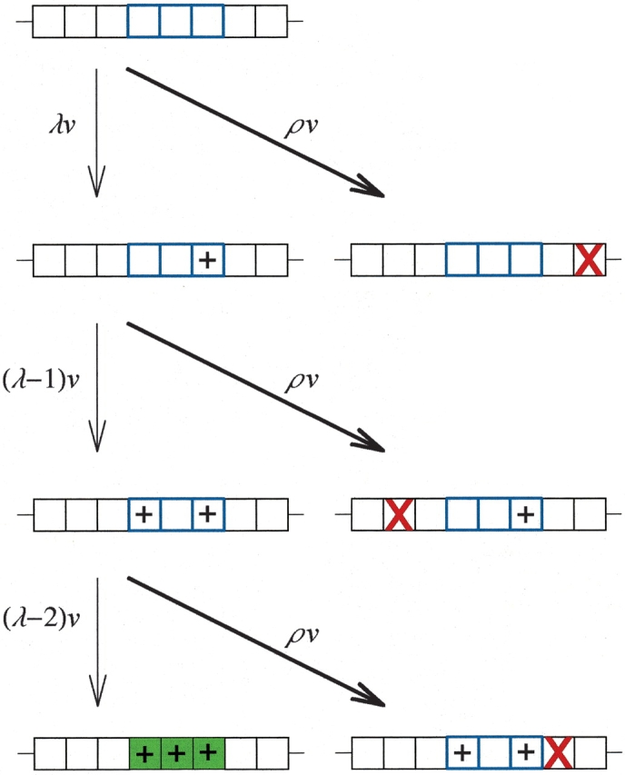
A freshly duplicated gene must accrue several compatible mutations without suffering a null mutation in order to code for the multiresidue (MR) feature. Each box in an array represents a nucleotide position in the duplicated gene. The three boxes outlined in blue are the positions that must be changed in order to produce the new MR feature. (Although they are contiguous in the drawing, they do not necessarily represent contiguous positions in the gene.) A “+” labels a compatible mutation. A red “X” labels a null mutation. The green-shaded box represents the gene coding for the MR feature, where the several necessary changes have all been acquired. The forward mutation rate is v times the number of incompatible loci λ remaining to be changed. The null mutation rate is ρv.

In our computer model of the process described above, the nucleotide positions that must be changed from the sequence of the parent gene to be compatible with the developing MR feature (we call states of nucleotide positions “compatible” if they are consistent with what is necessary to code for the MR feature, and “incompatible” if they are not) are explicitly represented as elements of an array (see Materials and Methods for details). These correspond to the squares outlined in blue in Figure 1 ▶. (Although the positions are next to each other in the figure, they are not necessarily contiguous in the gene.) These may be considered to be nucleotide positions in the same codon, separate codons, or a combination. The pertinent feature of the model is that multiple changes are required in the gene before the new, selectable feature appears. Changes in these nucleotide positions are assumed to be individually disruptive of the original function of the protein but are assumed either to enhance the original function or to confer a new function once all are in the compatible state. Thus, the mutations would be strongly selected against in an unduplicated gene, because its function would be disrupted and no duplicate would be available to back up the function.

The other nucleotide positions in the gene, corresponding to the black squares in Figure 1 ▶, which if they were changed would yield a null allele, are represented only implicitly in our computer model by the constant ρ, which is the ratio of the number of mutations of the original duplicated gene that would produce a null allele to the number of mutations of the original duplicated gene that would yield a compatible residue. (Definitions of terms are given in Table 1.) As an example, consider a gene of a thousand nucleotides. If a total of 2400 point mutations of those positions would yield a null allele, whereas three positions must be changed to build a new MR feature such as a disulfide bond, then ρ would be 2400/3, or 800. (Any possible mutations which are neutral are ignored.) In each generation of the simulation, each of the three positions that must be changed to yield the MR feature is sequentially given a chance to mutate with a probability governed by the mutation rate. However, although a mutation may occur in a position needed for an MR feature, it would nonetheless be unproductive if a null mutation had first occurred at a separate position. To simulate this possibility in our model, when an explicitly represented position does mutate, then we take a further probabilistic step to decide if a null mutation has in the meantime occurred elsewhere in the gene, in positions not explicitly represented. In the earlier example, if one of the three positions mutates, then a further step decides with probability ρ / (1 +ρ) (which in the example would be 800/801) that one or more null mutations have already occurred somewhere in the gene, and the gene is considered to be irrecoverably lost. (The likelihood of a null mutation reverting and the gene then successfully developing an MR feature before other null mutations occur is much lower than if the first λ mutations to the duplicate gene yield compatible residues; thus, we ignore that possibility.) With probability 1 / (1 +ρ) (in the example this would be 1/801), the gene is considered to be free of null mutations and continues in the simulation.

Table 1.

Definitions of terms

N	Number of organisms/duplicate genes in the population
λ	Number of initially incompatible nucleotide loci in a duplicate gene that must be changed to form the selectable, multiresidue feature
v	Point mutation rate per nucleotide per generation
ρ	Ratio of the number of possible mutations of the original duplicated gene that would produce a null allele to the number of possible mutations of the original duplicated gene that would yield a compatible residue. Neutral mutations, such as those that produce synonymous codons, are disregarded.
φ	Fraction of a particular nucleotide position that is in the incompatible state. (1 - φ) is the fraction in the compatible state.
t	Time, in generations
Tf	Time in generations to the first occurrence of a particular multiresidue, selectable features
Tfx	Time in generations to fixation in the population of a particular multiresidue, selectable feature
s	Selection coefficient

The starting point of the simulation (see Materials and Methods for a more complete description) is a population of organisms that already contains N exact duplicates of the parent gene, which then begin to undergo mutation. For simplicity, each position in an array, representing sites which must be changed to yield an MR feature, can be in either of just two states—the original incompatible state or the mutated, compatible state. Mutations can change a site either forward from incompatible to compatible or backward from compatible to incompatible. (Unlike for null mutations, reversions of compatible mutations back to incompatible ones must be explicitly considered because the probability of reversion in this case is significant.) These transitions occur with equal intrinsic probabilities.

Starting from a uniform population in which all sites that must be changed are in a state incompatible with the MR feature, then there are three processes in our model which affect the rate of approach of the population to steady state, which in turn affect the time required to generate the new MR feature:

1. Sites in the incompatible state can mutate to the compatible state before any null mutation has occurred. This takes place at a rate equal to the mutation rate per site times the fraction of sites that are in the incompatible state (since only that fraction can mutate directly to the compatible state) times the probability that no null mutation has already occurred. That is, at a rate equal to

   

   where v is the mutation rate per site per generation, φ is the fraction of nucleotide sites in the population that are in the incompatible state, ρ(as mentioned above) is the ratio of possible null to compatible mutations over the entire protein, and 1 / (1 +ρ) is the probability that a compatible mutation occurs before a null mutation. (Definitions of terms are given in Table 1.)

2. A site in the compatible state can mutate back to the incompatible state before a null mutation occurs. This takes place at a rate equal to

   

3. A mutation can occur in any one of the λ sites, but a stochastic check at this point decides with probability ρ / (1 +ρ) that one or more detrimental mutations have already occurred somewhere else in the protein, rendering it nonfunctional. The gene is then considered to be null, and it no longer counts in the model. However, the model allows for the occurrence of new gene duplication events, which recent estimates have shown to happen at a rate comparable to that of point mutation (Lynch and Conery 2000). Because the rates of point mutations and gene duplication are similar, in the model a gene that is determined to be null is replaced by a new gene duplication event, with a new copy of the original gene (which is presumed to be still under selection) with all sites in the original, incompatible state. In the computer model, this process effectively results in all λ sites of a null gene being reset to the original, incompatible state from whatever state they were in. This will happen at rate

   

   The number of nucleotide positions λ appears in this expression because the more compatible positions that were contained in a discarded null gene, the more that are replaced with incompatible ones in a new gene duplication event. The protocol of checking for null mutations in the model only when a mutation first occurs in one of the λ array sites has the intended effect of ensuring that gene duplication occurs in the population at a rate that is comparable to the rate of point mutation.

The overall net rate of change of the fraction φ of sites from the incompatible state will be a sum of these three processes:

(1)

The first term of the right-hand side of the equation is negative because it is a process in which incompatible sites are removed. The second and third terms are positive because they describe processes where incompatible sites are gained.

Integration yields:

(2)

The numerator of the right-hand term is the degree of saturation of the population with compatible mutations—the degree to which it has approached steady state. The value of (1 - φ) is the population-wide fraction of nucleotide positions that are in a state compatible with the MR feature.

Because of computing limitations, the values of 0.01–0.0001 used for the mutation rate v in the simulations presented following are much higher than the biologically realistic value of about 10⁻⁸ (Drake et al. 1998), and the values of 1–100 used here for ρ are lower than the value of a thousand or greater expected for biologically realistic situations (Walsh 1995). However, the fact that Figure 2 ▶ shows that the fraction (1 - φ) of compatible mutants in our simulations follows equation 2 very closely over a wide range of values for λ and ρ in populations that reproduce either deterministically or stochastically makes us more confident when we extrapolate the model to biologically realistic values of v andρ.

Figure 2.

Fraction (1-φ) of a nucleotide position in a compatible state versus time (generations) normalized for the mutation rate (vt). In all cases, the curves are determined from equation 2. (Top) N =10,000, v =0.001, deterministic reproduction. Circles: ρ=1, λ =2; inverted triangles: ρ=2, λ =3; squares: ρ=4, λ =5; diamonds: ρ=10, λ =10; triangles: ρ=100, λ =10. Each point is the average of 100 repetitions. (Bottom) N =100, v =0.001, ρ=1, λ =6. Circles are for deterministic reproduction; each point is the average of 100 repetitions. Triangles are for stochastic reproduction; each point is the average of 1024 repetitions.

In the following paragraphs, we develop from simple considerations an equation which gives the same quantitative behavior as the numerical model. In Appendix 1, we derive the same form of equation more rigorously by considering coupled equations representing different segments of the population.

What is the probability that a duplicated gene will give rise to a particular MR feature? Consider a gene with λ sites all originally in the incompatible state. As discussed previously, the probability of one of those sites mutating to a compatible state before the occurrence of a null mutation elsewhere in the gene is

Because any one of the λ sites can mutate first, we can write this as

To mutate another residue to a compatible state, we must choose among the remaining (λ- 1) possibilities. Thus, the probability for the second position is

The multiplied probability of all λ sites mutating to compatible states before a null mutation occurs and before a back mutation occurs is thus

(If a back mutation occurs at any point, the likelihood of successfully developing an MR feature is much lower than if the first λ mutations to the duplicate gene yield compatible residues; thus, we ignore that possibility.)

If the probability of an event is P, then of course on average 1/P opportunities will be required before the event occurs. Thus, to produce an MR feature in our model will require an average number of opportunities equal to the inverse of the probability discussed earlier, or

At steady state, the number of opportunities to produce an MR function in a given time period in a population will be equal to the number of point mutations that occur in the potential MR site across the population—that is, to the time multiplied by the mutation rate per nucleotide v, the number of nucleotide positions λ that must mutate to compatible residues, and the population size N —that is, equal to Nvλt. To produce a gene with λ compatible mutations, the incompatible residue in a gene with λ- 1 compatible mutations has to be mutated, so that the time to produce an MR function with λ compatible sites will be proportional to the degree of saturation of the system with genes containing λ- 1 compatible sites. However, as exemplified by Figure 2 ▶, our model does not start at steady state; it starts with all sites in the incompatible state. Thus, the time required to produce an event will also depend on the degree to which the system has approached steady state, as follows. If the degree of saturation for one compatible site is in general S, then the degree of saturation for n compatible sites is Sⁿ. Thus, the degree of saturation with λ- 1 compatible sites at any given time is equal to the degree of saturation given in equation 2 raised to the λ- 1 power. Because the degree of saturation changes in time, to find the total number of opportunities for producing an MR feature, this value must be integrated over time.

These considerations can be combined to yield a quantitative description of the behavior of the model with time. The expected average time T_f to the first occurrence of an MR feature for a population of duplicate genes initially in a uniform state, needing λ positions mutated to acquire the MR feature, and with a ratio λ of null-to-compatible mutations, can be evaluated by equation 3.

(3)

The right-hand side of equation 3 is the inverse of the probability discussed earlier. The left-hand side gives the number of opportunities for production of the MR feature in the nonequilibrium system starting with no nucleotide positions in compatible states. The preintegral term of the left-hand side of the equation, Nvλ, is the number of point mutations occurring in the population per unit time at steady state. The integrand of equation 3, which is the numerator from the right-hand side of equation 2 raised to the power of λ- 1, is the degree of saturation of the system with “preselectable” mutants—that is, mutants that are one step from being selectable, with λ- 1 sites in the compatible state.

Figure 3 ▶ shows the result of simulations in which the number of sites λ in an MR feature was varied along with the ratio ρ of null-to-compatible mutations and the haploid population size N. As can be seen, the curves generated by equation 3 match the results of the simulations very closely for a wide range of values of N, ρ, and λ.

Figure 3.

Normalized time (generations) to first appearance (vT_f) versus number of loci λ required to be changed to yield the multiresidue (MR) feature. In all cases, the curves are determined from equation 3. v =0.01. Reproduction was deterministic. Filled circles, N =1; open circles, N =10; filled inverted triangles, N =100; open inverted triangles circles, N =1000; filled squares, N =10,000; open squares, N =100,000. (Upper left) ρ=1; (upper right) ρ =2; (lower left) ρ =4; (lower right) ρ =10. Each point is the average of 100 repetitions.

The effect of selection

The simulations shown in Figure 3 ▶ examined the number of generations required to produce just the first occurrence of an MR feature in a population. However, beneficial mutations are frequently lost from a population by stochastic processes before fixation (Kimura 1983). In Figure 4 ▶, we present the results of simulations which determine the time to fixation T_fx of the MR feature in the population as a function of the strength of the selection coefficient s. The simulation results are well fit by equation 4.

Figure 4.

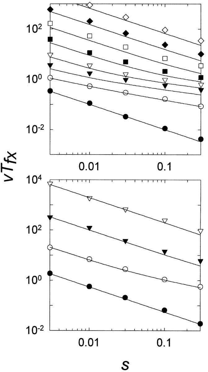
Normalized time (generations) to fixation (^vTfx^{) versus the se}lection coefficient s. In all cases, the curves are determined from equation 4. Reproduction was stochastic. N =1000; v =0.01–0.0001. Each point is the average of 100 repetitions. (Top) ρ=1. Filled circles, λ =1; open circles, λ =2; filled inverted triangles, λ =3; open inverted triangles circles, λ =4; filled squares, λ =5; open squares, λ =6; filled diamonds, λ =7; open diamonds, λ =8. (Bottom) ρ=10. Filled circles, λ =1; open circles, λ =2; filled inverted triangles, λ =3; open inverted triangles, λ =4.

(4)

Equation 4 is a minor modification of equation 3, where the right-hand side of the equation is divided by twice the selection coefficient. This result follows from the dependence of the fixation probability on the selection coefficient (Li 1997).

Pre-equilibration of the population

Thus far, the starting point for the model has been a uniform population in which all genes are initially present as exact duplicates of the parent gene. Mutations then begin to accumulate and the program immediately starts to check for the presence of the MR feature, simulating the presence of selective pressure from the start. However, a different situation can also be considered, in which the duplicate gene begins to undergo mutation, but selective pressure arises only at a later time, perhaps as a result of environmental changes. In that case, the population of duplicate genes will be at least part of the way toward its steady-state frequency before selection affects the population. This can be modeled in the simulation by neglecting to check for the presence of the MR feature, treating it as a neutral property, until a predetermined number of generations have passed.

Figure 5 ▶ shows the result of simulations in which all duplicate genes began in a uniform state, identical to the parent gene, but the population was allowed to undergo mutation and reproduction for varying periods of time before starting to check for the MR feature. It can be seen that as the length of the pre-equilibration period increases, the average time from the start of selection to observation of the duplicate gene coding for the new MR feature decreases for population sizes, where, at steady state in the absence of selection, at least one duplicated gene with the feature is expected to already be present in the population, that is, where the population size is greater than the inverse of the probability of producing the MR feature, N > (1 +ρ)^λ(λ^λ/λ!). In Figure 5 ▶, this occurs at λ ≤ 5. For the case where N < (1 +ρ)^λ(λ^λ/λ!) (at λ ≥ 6 in Fig. 5 ▶), however, the expected time is essentially unaffected by pre-equilibration of the population. Because it follows from equation 3 that N < (1 +ρ)^λ(λ^λ/λ!), when v times the evaluated integral is >1, then T_f will be substantially unaffected by pre-equilibration when T_f ≥ 1 / v.

Figure 5.

Effect of pre-equilibration of the population on normalized time (generations) to first appearance (vT_f) versus number of loci λ required to be changed to yield the MR feature. N =1000; v =0.001; ρ=1. Each point is the average of 100 repetitions. The curve is determined from equation 3. Reproduction was deterministic. The simulation was pre-equilibrated (that is, the population was subject to mutation and reproduction without checking for the appearance of the multiresidue (MR) feature, regarding it as neutral) for filled circles, 0 generations; open circles, 0.1 / v generations; filled inverted triangles, 0.3 / v generations; open inverted triangles, 1 / v generations; filled squares, 3 / v generations.

Discussion

The model and its limits

Some features of proteins, such as disulfide bonds and ligand binding sites, which here we call MR features, are composed of multiple amino acid residues. As Li (1997) points out, the evolutionary origins of such features must have involved multiple mutations that were initially neutral with respect to the MR feature. We have attempted to model such a process. In doing so, one might examine a number of possible routes to an MR feature, for example, looking at a unique gene that is under selective constraints, or looking at mutations caused by insertions and deletions or recombination in a duplicate gene. Our model is restricted to the development of MR features by point mutation in a duplicated gene. We strongly emphasize that results bearing on the efficiency of this one pathway as a conduit for Darwinian evolution say little or nothing about the efficiency of other possible pathways. Thus, for example, the present study that examines the evolution of MR protein features by point mutation in duplicate genes does not indicate whether evolution of such features by other processes (such as recombination or insertion/deletion mutations) would be more or less efficient.

There are several reasons, both practical and theoretical, for examining this limited model. First, as mentioned earlier, gene duplication is considered to be a major route to evolutionary novelty (Ohno 1970; Lynch and Conery 2000; Wagner 2001; Chothia et al. 2003) and therefore it is important to explore its potential in regard to MR features. Second, a duplicated gene can be considered to be largely free of the effects of purifying selection (but see following) and therefore selective effects, which are difficult to estimate, can be ignored, simplifying the task at hand. Third, point mutations are well-defined events, where transitions occur among a limited set of states. In contrast, insertions and deletions vary in size and composition, making them difficult to model for our purposes. Thus, we confine our model of the development of MR features to what we consider to be the conceptually simplest and computationally most tractable route, of point mutations in a duplicated gene that is free of purifying selection.

Is the assumption of the selective neutrality of duplicated genes either a realistic or a useful one? On the one hand, the assumption appears not to be correct in at least some situations. For example, although the vast majority of neutral duplicated genes are expected to result in null alleles, studies of polyploid organisms showed that more duplicate genes survived over long periods of time than expected (Ferris and Whitt 1977, 1979; Hughes and Hughes 1993; White and Doebley 1998). This has provoked the suggestion that gene dosage effects in polyploids might slow the decay of duplicate gene copies and that more duplicates may be preserved than expected by the process of subfunctionalization, where a gene with two or more functions duplicates and each copy subsequently loses one of the functions and then goes on to specialize in the preserved function (Force et al. 1999; Lynch et al. 2001). Although the assumption of the selective neutrality of duplicated genes does not fit data from some polyploid species (Ferris and Whitt 1977, 1979; Hughes and Hughes 1993; White and Doebley 1998), it may yet be a good model for individual gene duplication events (Lynch and Conery 2000). In support of this view, recent studies have shown that genes that have been recently duplicated seem to be under relaxed selection, as indicated by the similar number of synonymous and nonsynonymous mutations they have acquired (Lynch and Conery 2000; Kondrashov et al. 2002).

On the other hand, it should be emphasized that the utility of the idealized model presented here—where there is no selective effect from duplicate genes or from intermediate states of the gene until the MR feature is completely in place in a gene and where the only mutagenic process considered is point mutations—is not dependent on a comprehensive accounting for all relevant biological processes. Rather, its usefulness lies in its ability to indicate when processes in addition to those described in the model are required to account for a feature. If the development of an MR feature by means of point mutation in an ideal, neutral, duplicated gene would require unrealistically large population sizes or unrealistically long times, then one can conclude that other factors (such as recombination, selection of intermediate states, and/or other factors) must be examined to account for the feature. Because neutral gene duplication and point mutation is often invoked to account for complex features of proteins, it would be useful to have a quantitative understanding for what such scenarios would entail in order to assess their reasonableness.

In our simulations, the model starts in a uniform initial state, with the population already in possession of N exact duplicates of the parent gene. This, of course, is biologically unrealistic but can be considered to approximate the end result of either of two processes: (1) the spread of a duplicate gene through a population by random drift until it is fixed or (2) the occurrence of a phylogenetic branching point, where after the branch point, a small population that is homogeneous with respect to the duplicate gene expands to a population size N. Although mutations will occur in copies of the duplicate gene during the period of either drift of the gene or expansion of the population, there will be fewer mutations—and thus fewer opportunities to produce the MR feature—than in a population already at size N, each with on average one copy of the duplicate gene, for the same period of time. In either case, the time to reach the initial state is neglected, so the time obtained from the simulations can be considered to be an underestimate of the time to fixation T_fx of the MR feature. Although we envision each organism of the population as having one duplicate gene per haploid genome, because recombination is disallowed and each duplicate accumulates mutations independently, it does not affect the model (as represented by equation 4) if there is variation in copy number of the duplicate gene in organisms, as long as the total number of duplicate gene copies in the population is N.

Figure 3 ▶ shows that the results of the simulation closely match those predicted from equation 3, which gives us confidence to extrapolate to biologically realistic values of the parameters of the equation. The curves in Figure 3 ▶ exhibit two regions: (1) a nonlinear region at larger population sizes and/or smaller numbers of sites and (2) a linear region at smaller population sizes and/or higher numbers of loci. These regions represent, respectively, (1) the situation where in the absence of selection for the MR feature the steady-state population would be expected to contain one or more copies of the duplicate gene with an MR feature [that is, where N > (1 +ρ)^λ(λ^λ/λ!)] and (2) the situation where in the absence of selection, the population on average at steady state is not expected to contain a copy with the MR feature [that is, where N < (1 +ρ)^λ(λ^λ/λ!)].

The expected time for the nonlinear region largely reflects the amount of time necessary for the population to approach steady state. This time is on the order of the inverse of the rate of point mutation and is relatively insensitive to either the number of loci involved in the MR feature or the population size, varying inversely with only the λ^th root of N (see Appendix 2). Thus, the ability to decrease the time required to produce an MR feature much below 1 / v by increasing population size is greatly constrained by the nonlinearity of the model, reflecting the slow equilibration of the population when multiple mutations are required.

As shown in Figure 4 ▶, the effect of changes in the selection coefficient on the behavior of the model are closely fit by equation 4. It should be noted that the time calculated from equation 4 reflects the average time required simply to produce the MR mutant that will go on to become fixed in the population; it does not explicitly include the time required for the mutation to spread and become fixed in the population once it has been produced. The close fit of the simulation results of Figure 4 ▶—which does include both the time to produce the MR mutation that will be fixed plus the time required for the mutation to spread through the population to fixation—to the curve predicted from equation 4 emphasizes the fact that the timescale for fixation of the mutation is negligible compared with the timescale required to produce the mutation that will go on to become fixed.

As shown in Figure 5 ▶ for the nonlinear region, if the population has been accumulating mutations for a period of time before selection for the MR feature is applied (perhaps representing a population approaching steady state where the environment then changes, making a feature selectable that previously had been neutral), then the expected time, measured from the start of selection to the appearance of the MR feature, decreases. On the other hand, as also shown in Figure 5 ▶, for situations where the population is not expected to have a copy of the duplicate gene with the MR feature at steady state (in Figure 5 ▶, for λ ≥ 6), then the expected time to its fixation is essentially unaffected by pre-equilibration of the population. This is the case whenever T_f ≥ 1 / v. It should be noted that pre-equilibration explicitly allows for the occurrence of rare, “lucky” alleles whose sequence is closer to that of the MR feature than is the sequence of the starting, predominant gene. Such rare alleles could thus be poised to give rise to the MR feature in perhaps one or two steps. The result shown in Figure 5 ▶—that, for λ ≥ 6, pre-equilibration has no effect on T_f—demonstrates that on average the opportunity for the serendipitous occurrence of rare alleles does not alter the expected time.

Estimation of T_fx for several cases

Estimated values for parameters of our model can be garnered from the literature. Drake et al. (1998) estimate the deleterious mutation rate to be about 0.2–2.0 per generation per effective genome size of 10⁸ bp for a variety of multicellular organisms, both vertebrate and invertebrate. We use that number to approximate the effective nucleotide point mutation rate per generation v in coding regions to be on the order of 10⁻⁸. Lynch and Conery (2000) calculate the rate of duplication of a given gene to be 0.01 per million years—in other words, 10⁻⁸ per year, which for our purposes we consider to be roughly equal to the estimated nucleotide point mutation rate (Lynch and Conery 2000; see also the discussion of that work [Long and Thornton 2001; Lynch and Conery 2001; Zhang et al. 2001]). Although here we assign single values to the parameters, one must keep in mind that there is significant uncertainty in estimating them and that the rates may vary with time, species, region of the genome, and other factors.

An estimate of ρ can be inferred from studies of the tolerance of proteins to amino acid substitution. Although there is variation among different positions in a protein sequence, with surface residues in general being more tolerant of substitution than buried residues, it can be calculated that on average a given position will tolerate about six different amino acid residues and still maintain function (Reidhaar-Olson and Sauer 1988, 1990; Bowie and Sauer 1989; Lim and Sauer 1989; Bowie et al. 1990; Rennell et al. 1991; Axe et al. 1996; Huang et al. 1996; Sauer et al. 1996; Suckow et al. 1996). Conversely, mutations to an average of 14 residues per site will produce a null allele, that is, one coding for a nonfunctional protein. Thus, in the coding sequence for an average-sized protein domain of 200 amino acid residues, there are, on average, 2800 possible substitutions that lead to a nonfunctional protein as a result of direct effects on protein structure or function. If several mutations are required to produce a new MR feature in a protein, then ρ is roughly of the order of 1000. This value for ρ is on the low end used by Walsh (1995), who considered values for ρ up to 10⁵. (Walsh, however, defined ρ as the ratio of advantageous-to-null mutations—the inverse of our definition.)

It should be emphasized that the value of ρ is not the ratio of mutations to an organismal genome that would be lethal to those that would be mildly deleterious. Rather, it is the ratio of the number of mutations that would inactivate a typical protein to the number that would lead to a new MR feature for that particular protein. Many genes can be silenced with small or moderate ill effect on the organism (for example, the gene for myoglobin can be inactivated in mice with little ill effect in adult mice [Garry et al. 1998 for example, the gene for myoglobin can be inactivated in mice with little ill effect in adult mice [Garry et al. 2003; Meeson et al. 2001]). However, if a mutation inactivates a protein, then it is counted in the model as a null mutation for purposes of calculating ρ, whether or not it may have severe phenotypic effects. The best estimate for this number comes not from studies of mutations in organisms, but rather from studies of the tolerance of specific proteins to mutation (Reidhaar-Olson and Sauer 1988, 1990; Bowie and Sauer 1989; Lim and Sauer 1989; Bowie et al. 1990; Rennell et al. 1991; Axe et al. 1996, 1998; Huang et al. 1996; Sauer et al. 1996; Suckow et al. 1996).

The uncertainties involved in estimating ρ should be kept in mind. On the one hand, although as just discussed, studies selecting for activity of mutant proteins show most substitutions to reduce function below that required for a biological assay, a study searching for inactivating mutations to the autotoxic ribonuclease barnase showed that comparatively few substitutions reduced activity to that of uncatalyzed reactions (Axe et al. 1998). This consideration may lower the estimate of ρ. On the other hand, duplicate genes might also be lost by processes other than point mutation, such as deletion or recombination. Additionally, null mutations in the coding sequence or flanking sequences might occur because of indirect effects such as, for example, altering the stability of the mRNA. These considerations might effectively increase the value of ρ.

Figure 6 ▶ uses equation 4 and the values for v and ρ estimated earlier to plot the expected time in generations to the fixation of an MR protein feature for populations of different sizes. In addition, we use a value of 0.01 for the selection coefficient s. Figure 6 ▶ shows that the fixation of specific MR features by point mutation in duplicated genes is a long-term phenomenon that requires populations of considerable size. For example, consider a case where three nucleotide changes must be made to generate a novel feature such as a disulfide bond. In that instance, Figure 6 ▶ shows that a population size of approximately 10¹¹ organisms on average would be required to give rise to the feature over the course of 10⁸ generations, and this calculation is unaffected by pre-equilibration of the population in the absence of selection. To produce the feature in one million generations would, on average, require an enormous population of about 10¹⁷ organisms, although this number would change if the population had pre-equilibrated in the absence of selection.

Figure 6.

Time to fixation T_fx versus number of loci λ required to be changed to yield the multiresidue (MR) feature. v =10⁻⁸; ρ=1000; s =0.01. Values for population sizes N are given across the top axis. In all cases the curves are determined from equation 4. A line is drawn across the figure at T_fx = 1 / v, which is 108 generations. Above the line, values for T_fx are essentially unaffected by pre-equilibration of the population in the absence of selection.

For features requiring more participating residues, the expected population sizes are even larger. As Li (1997) noted, the binding site for diphosphoglycerate in hemoglobin requires three residues. The population size required to produce an MR feature consisting of three interacting residues by point mutation in a duplicated gene initially lacking those residues would depend on the number of nucleotides that had to be changed—a minimum of three and a maximum of nine. If six mutations were required then, as indicated by Figure 6 ▶, on average a population size of ~1022 organisms would be necessary to fix the MR feature in 10⁸ generations, and a population of ~1030 organisms would be expected to fix the mutation in one million generations. In a recent in vitro study intended to mimic evolution, a recombinant amphioxus insulin-like peptide was altered by site-directed mutagenesis at seven nucleotide positions to contain five altered amino acid residues that would allow interaction with mammalian insulin receptor (Guo et al. 2002). In order for such a process to occur in vivo by gene duplication and point mutation within a hundred million generations would be expected on average to require >10²⁵ organisms.

Such numbers seem prohibitive. However, we must be cautious in interpreting the calculations. On the one hand, as discussed previously, these values can actually be considered underestimates because they neglect the time it would take a duplicated gene initially to spread in a population. On the other hand, because the simulation looks for the production of a particular MR feature in a particular gene, the values will be overestimates of the time necessary to produce some MR feature in some duplicated gene. In other words, the simulation takes a prospective stance, asking for a certain feature to be produced, but we look at modern proteins retrospectively. Although we see a particular disulfide bond or binding site in a particular protein, there may have been several sites in the protein that could have evolved into disulfide bonds or binding sites, or other proteins may have fulfilled the same role. For example, Matthews’ group engineered several nonnative disulfide bonds into lysozyme that permit function (Matsumura et al. 1989). We see the modern product but not the historical possibilities.

We should also notice which parameters the model is particularly sensitive to and which not. The model is least sensitive to the point mutation rate v and the selection coefficient s because both of those appear only as linear terms in equation 4. Thus, for example, if we consider an organism where the point mutation rate is increased by a factor of 10³, then the numbers calculated from equation 4 will decrease by only that factor. For the case discussed earlier in which six nucleotide changes were required, the population size needed to fix the feature in 10⁸ generations would then decrease from 10²² to just 10¹⁹.

The model is more sensitive to the value ofρ, because ρ appears with an exponent in equation 4. If ρ were less by a factor of 10 (100 instead of 1000), then the population size needed to fix the feature in the preceding example in 10⁸ generations would decrease from 10²² to 10¹⁶. The number of possible null mutations—the numerator ofρ—arises from basic considerations of protein structure so that it is unlikely to vary significantly. The number of possible compatible mutations λ—the denominator ofρ—is more difficult to estimate. However, the value of one thousand that we use for ρ in Figure 6 ▶ is conservative compared with the range of values used by other workers (Walsh 1995). It should be noted that as λ becomes larger, the number of possible null mutations—and thus implicitly the length of the gene—must increase to maintain a constant value ofρ.

The model is most sensitive to the value of λ—the number of loci that must mutate before a new MR function occurs—which appears as an exponent in equation 4. If in the case just mentioned, because of the particular initial sequence of the parent gene, either three or nine nucleotide changes were necessary instead of six, then the population sizes required to fix the feature in 10⁸ generations would vary from 10¹¹ to 10³¹ organisms. The dependence on λ may encourage speculation that perhaps MR mutations could develop by point mutation in duplicate genes if the parent gene giving rise to the duplication were serendipitously poised to lead to the new feature with only one mutation in the precursor gene. Although this is certainly possible, it is unlikely to be the general case. As one example, Li (1997) has argued that the precursor to modern hemoglobins that can bind diphosphoglycerate did not have any of the three amino acid residues involved in the interaction. As shown in Figure 5 ▶, for the average case, pre-equilibration, which allows for the occurrence of rare, fortunate alleles, does not affect the expected time T_f in the linear portion of the curve.

The lack of recombination in our model means it is most directly applicable to haploid, asexual organisms. Nonetheless, the results also impinge on the evolution of diploid sexual organisms. The fact that very large population sizes—10⁹ or greater—are required to build even a minimal MR feature requiring two nucleotide alterations within 10⁸ generations by the processes described in our model, and that enormous population sizes are required for more complex features or shorter times, seems to indicate that the mechanism of gene duplication and point mutation alone would be ineffective, at least for multicellular diploid species, because few multicellular species reach the required population sizes. Thus, mechanisms in addition to gene duplication and point mutation may be necessary to explain the development of MR features in multicellular organisms.

Although large uncertainties remain, it nonetheless seems reasonable to conclude that, although gene duplication and point mutation may be an effective mechanism for exploring closely neighboring genetic space for novel functions, where single mutations produce selectable effects, this conceptually simple pathway for developing new functions is problematic when multiple mutations are required. Thus, as a rule, we should look to more complicated pathways, perhaps involving insertion, deletion, recombination, selection of intermediate states, or other mechanisms, to account for most MR protein features.

Materials and methods

A duplicated gene in a population was represented by an array of integer elements that could take the values of either zero or one. The number of elements λ in the array corresponded to the number of nucleotide positions that would have to mutate in a particular gene to yield a hypothesized MR protein feature. In all cases, we begin the simulation in a uniform initial state, with N duplicate copies of the parent gene in the population, represented by N identical arrays. This simplification of starting with the duplicate gene already fixed in the population ignores the time needed for the duplicate copy to initially spread in the population; thus the average times we calculate from this model can be considered underestimates of the time for fixation of a gene with a new MR function. All elements of the array were initially set to a value of one, which represented the initial, incompatible state of the position, which could not contribute to the MR feature. Each position in an array was then allowed to mutate sequentially with a probability set by the mutation rate v. A value of zero represented the state that could potentially contribute to an MR feature. Back mutations were permitted, so that a position with a value of zero could revert to a value of one. The equal rates of forward and backward point mutations should not be confused with the very different rates at which a gene will acquire null mutations versus acquiring a new, selectable MR feature.

After each step in which a mutation occurred at an array position, a further probabilistic step was taken to simulate the possible occurrence of one or more null mutations elsewhere in the gene. With probability 1 / (1 +ρ), where ρ is the ratio of null-to-compatible mutations in the gene (neutral mutations are ignored), the gene was considered to be free of null mutations and continued in the simulation. With probability ρ / (1 +ρ) the gene was deemed to have suffered one or more null mutations at positions not explicitly represented in the array and consequently to have become a pseudogene. In this case, the array was replaced in the population by a new array in which all loci were again set to one. This is intended to simulate replacement of the nonfunctional duplicate gene by a new duplication of the original gene, whose sequence is considered to remain constant under selection. Checking for null mutations only when mutations occur at an array position has the intended effect of making the gene duplication rate similar to the rate of point mutation v. It has recently been shown that those two rates are in fact similar (Lynch and Conery 2000). It should be noted that the model purposely does not replace the duplicate gene immediately whenever a null mutation would occur anywhere in the gene, rather than waiting for one of the λ array sites to mutate, because that would have the effect of making the gene duplication rate much faster than it is estimated to be.

After the mutation step, the population was checked for the number of selectable organisms—those whose array elements all had a value of zero. Arrays in which some but not all elements were in a compatible state had no advantage. (This models MR features where, by hypothesis, the selectable feature does not exist until all contributing amino acids are in the correct state.) For most simulations, the run was halted when the first selectable array was discovered and the time in generations to the first occurrence of the selectable MR mutant recorded. For other runs, the simulation was continued and selection was applied at the reproduction step. In these cases, the simulation was continued until >50% of the population carried the MR feature, which was then considered to be “fixed” in the population, and the time to fixation recorded. The time for the selectable MR mutation to spread is generally much less than the time for it to be produced by the population.

After each array was subjected to the mutation step, the next generation was populated, either by deterministic reproduction or by simulated stochastic reproduction. In deterministic reproduction, the next generation was taken clonally from the previous; that is, the composition of the next generation was identical to the previous generation after the mutation step. In stochastic reproduction, the subsequent generation was populated by copying randomly chosen arrays, with or without selection, from the previous generation until the subsequent generation was fully populated.

In some simulations, the process was “prerun” for a selected number of generations, undergoing mutation and reproduction but not selection. This was done to model populations that had to varying degrees approached steady state with respect to the occurrence of the MR mutation in the population in the absence of selection for it.

All equations were evaluated using Mathematica.

Abbreviations

• MR, multiresidue

Appendix 1

Consider a population in which the number of duplicated genes that has none of the necessary mutations to produce an MR feature is n₀, the number that has one required mutation is n₁, the number with two required mutations is n₂, and so forth. As in the text, v is the mutation rate per nucleotide per generation, ρis the ratio of possible null mutations to compatible mutations in a gene, and λ is the number of initially incompatible nucleotide loci in a duplicate gene that must be changed to form the selectable, MR feature. Also as in the text, genes suffering a null mutation are presumed to be replaced by a new duplicate of the original gene, with all loci in the incompatible state. Then we can write:

(5)

(6)

(7)

(8)

where

and

Terms representing processes in which an additional compatible mutation is gained without a null mutation first occurring are multiplied by the factor λ- m, where m is the number of compatible mutations a gene has already acquired, to account for the decreasing number of sites that are available for potentially beneficial mutation, and terms representing processes in which a compatible mutation is lost without a null mutation first occurring are multiplied by m to account for the increasing number of sites that can revert. Equation 8 represents the transition to an absorbing state that is under selection, where all required mutations necessary for the new MR feature are present. Once in the selectable state, the gene is presumed not to leave by mutation to another state. (This is similar to the situation described by equation 3, where the time to just the first appearance of an MR feature is estimated, which thus does not allow for back mutation of the gene with the MR feature.)

If ρ ≫ 1, then n₀ ≫ n₁ ≫ n₂…and β ≫ α. In this limit, equations 5–8 become simply:

(9)

(10)

(11)

(12)

These can be solved in sequence by successive approximations. For equation 10, we approximate n₀ ≈ N (the total population size), which for initial condition n₁ = 0 gives:

(13)

which has the solution

(14)

Using this solution for n₁ in the next equation, with initial condition n₂ = 0, we have

(15)

Therefore, using the same approximation successively, we obtain

(16)

Last, we integrate equation 16 to get nλ. Setting nλ =1 (the first appearance of the MR feature) yields

(17)

or

(18)

When ρ is small (<10), the values of T_f given by equation 18 do not give a good match to the results of the simulations, which are nonetheless closely matched by equation 3 in the text. When ρ is large (≥10), however, which will be the case in biologically realistic situations, then equation 18 is approximately equal to equation 3 and both equations closely match the results of the simulations because, for largeρ, for the exponent of the integrand on the left-hand sides of the equations

and for the right-hand sides of the equations

Appendix 2

In the limit of T_f ≪ 1 / vλ, the left-hand sides of both equation 3 and equation 18 are proportional to (T_f)λ. This is seen in the following:

(19)

(20)

(21)

where γ ≈ vλ for both equations in the limit ρ ≫ 1. In this limit, equations 3 and 18 therefore become

(22)

which implies

(23)

where we have used the approximations of Appendix 1 for the case of ρ ≫ 1. The limit T_f ≪ 1 / vλ therefore corresponds to the limit N ≫ (1 +ρ)^λ(λ^λ/λ!), or ρ ≪ N^{1 / λ}.

For ρ ≪ N^{1 / λ}, then, the time required to produce a selectable state is inversely proportional to the λ^th root of the population size, that is, T_f∞N^{(−1 / λ)}.

Article published online ahead of print. Article and publication date are at http://www.proteinscience.org/cgi/doi/10.1110/ps.04802904.

References

- Axe, D.D., Foster, N.W., and Fersht, A.R. 1996. Active barnase variants with completely random hydrophobic cores. Proc. Natl. Acad. Sci. 93 5590–5594. [DOI] [PMC free article] [PubMed] [Google Scholar]
- ———. 1998. A search for single substitutions that eliminate enzymatic function in a bacterial ribonuclease. Biochemistry 37 7157–7166. [DOI] [PubMed] [Google Scholar]
- Bowie, J.U. and Sauer, R.T. 1989. Identifying determinants of folding and activity for a protein of unknown structure. Proc. Natl. Acad. Sci. 86 2152–2156. [DOI] [PMC free article] [PubMed] [Google Scholar]
- Bowie, J.U., Reidhaar-Olson, J.F., Lim, W.A., and Sauer, R.T. 1990. Deciphering the message in protein sequences: Tolerance to amino acid substitutions. Science 247 1306–1310. [DOI] [PubMed] [Google Scholar]
- Braden, B.C. and Poljak, R.J. 1995. Structural features of the reactions between antibodies and protein antigens. FASEB J. 9 9–16. [DOI] [PubMed] [Google Scholar]
- Chakrabarti, P. and Janin, J. 2002. Dissecting protein-protein recognition sites. Proteins 47 334–343. [DOI] [PubMed] [Google Scholar]
- Chothia, C., Gough, J., Vogel, C., and Teichmann, S.A. 2003. Evolution of the protein repertoire. Science 300 1701–1703. [DOI] [PubMed] [Google Scholar]
- Cunningham, B.C. and Wells, J.A. 1993. Comparison of a structural and a functional epitope. J. Mol. Biol. 234 554–563. [DOI] [PubMed] [Google Scholar]
- Drake, J.W., Charlesworth, B., Charlesworth, D., and Crow, J.F. 1998. Rates of spontaneous mutation. Genetics 148 1667–1686. [DOI] [PMC free article] [PubMed] [Google Scholar]
- Ferris, S.D. and Whitt, G.S. 1977. Loss of duplicate gene expression after polyploidisation. Nature 265 258–260. [DOI] [PubMed] [Google Scholar]
- ———. 1979. Evolution of the differential regulation of duplicate genes after polyploidization. J. Mol. Evol. 12 267–317. [DOI] [PubMed] [Google Scholar]
- Force, A., Lynch, M., Pickett, F.B., Amores, A., Yan, Y.L., and Postlethwait, J. 1999. Preservation of duplicate genes by complementary, degenerative mutations. Genetics 151 1531–1545. [DOI] [PMC free article] [PubMed] [Google Scholar]
- Garry, D.J., Ordway, G.A., Lorenz, J.N., Radford, N.B., Chin, E.R., Grange, R.W., Bassel-Duby, R., and Williams, R.S. 1998. Mice without myoglobin. Nature 395 905–908. [DOI] [PubMed] [Google Scholar]
- Garry, D.J., Kanatous, S.B., and Mammen, P.P. 2003. Emerging roles for myoglobin in the heart. Trends Cardiovasc. Med. 13 111–116. [DOI] [PubMed] [Google Scholar]
- Guo, Z.Y., Shen, L., Gu, W., Wu, A.Z., Ma, J.G., and Feng, Y.M. 2002. In vitro evolution of amphioxus insulin-like peptide to mammalian insulin. Biochemistry 41 10603–10607. [DOI] [PubMed] [Google Scholar]
- Huang, W., Petrosino, J., Hirsch, M., Shenkin, P.S., and Palzkill, T. 1996. Amino acid sequence determinants of β-lactamase structure and activity. J. Mol. Biol. 258 688–703. [DOI] [PubMed] [Google Scholar]
- Hughes, M.K. and Hughes, A.L. 1993. Evolution of duplicate genes in a tetraploid animal, Xenopus laevis. Mol. Biol. Evol. 10 1360–1369. [DOI] [PubMed] [Google Scholar]
- Janin, J. and Chothia, C. 1990. The structure of protein-protein recognition sites. J. Biol. Chem. 265 16027–16030. [PubMed] [Google Scholar]
- Kimura, M. 1983. The neutral theory of molecular evolution. Cambridge University Press, Cambridge, UK.
- Kondrashov, F.A., Rogozin, I.B., Wolf, Y.I., and Koonin, E.V. 2002. Selection in the evolution of gene duplications. Genome Biol. 3 RESEARCH0008. [DOI] [PMC free article] [PubMed] [Google Scholar]
- Li, W.H. 1997. Molecular evolution. Sinauer Associates, Sunderland, MA.
- Lim, W.A. and Sauer, R.T. 1989. Alternative packing arrangements in the hydrophobic core of λ repressor. Nature 339 31–36. [DOI] [PubMed] [Google Scholar]
- Lo, C.L., Chothia, C., and Janin, J. 1999. The atomic structure of protein-protein recognition sites. J. Mol. Biol. 285 2177–2198. [DOI] [PubMed] [Google Scholar]
- Long, M. and Thornton, K. 2001. Gene duplication and evolution. Science 293 1551. [DOI] [PubMed] [Google Scholar]
- Lynch, M. and Conery, J.S. 2000. The evolutionary fate and consequences of duplicate genes. Science 290 1151–1155. [DOI] [PubMed] [Google Scholar]
- ———. 2001. Gene duplication and evolution. Science 293 1551. [DOI] [PubMed] [Google Scholar]
- Lynch, M. and Walsh, B. 1998. Genetics and analysis of quantitative traits. Sinauer, Sunderland, MA.
- Lynch, M., O’Hely, M., Walsh, B., and Force, A. 2001. The probability of preservation of a newly arisen gene duplicate. Genetics 159 1789–1804. [DOI] [PMC free article] [PubMed] [Google Scholar]
- Matsumura, M., Becktel, W.J., Levitt, M., and Matthews, B.W. 1989. Stabilization of phage T4 lysozyme by engineered disulfide bonds. Proc. Natl. Acad. Sci. 86 6562–6566. [DOI] [PMC free article] [PubMed] [Google Scholar]
- Meeson, A.P., Radford, N., Shelton, J.M., Mammen, P.P., DiMaio, J.M., Hutcheson, K., Kong, Y., Elterman, J., Williams, R.S., and Garry, D.J. 2001. Adaptive mechanisms that preserve cardiac function in mice without myoglobin. Circ. Res. 88 713–720. [DOI] [PubMed] [Google Scholar]
- Ohno, S. 1970. Evolution by gene duplication. Springer-Verlag, Berlin, Germany.
- Ohta, T. 1987. Simulating evolution by gene duplication. Genetics 115 207–213. [DOI] [PMC free article] [PubMed] [Google Scholar]
- ———. 1988a. Further simulation studies on evolution by gene duplication. Evolution 42 375–386. [DOI] [PubMed] [Google Scholar]
- ———. 1988b. Time for acquiring a new gene by duplication. Proc. Natl. Acad. Sci. 85 3509–3512. [DOI] [PMC free article] [PubMed] [Google Scholar]
- Reidhaar-Olson, J.F. and Sauer, R.T. 1988. Combinatorial cassette mutagenesis as a probe of the informational content of protein sequences. Science 241 53–57. [DOI] [PubMed] [Google Scholar]
- ———. 1990. Functionally acceptable substitutions in two α-helical regions of λ repressor. Proteins 7 306–316. [DOI] [PubMed] [Google Scholar]
- Rennell, D., Bouvier, S.E., Hardy, L.W., and Poteete, A.R. 1991. Systematic mutation of bacteriophage T4 lysozyme. J. Mol. Biol. 222 67–88. [DOI] [PubMed] [Google Scholar]
- Sauer, R.T., Milla, M.E., Waldburger, C.D., Brown, B.M., and Schildbach, J.F. 1996. Sequence determinants of folding and stability for the P22 Arc repressor dimer. FASEB J. 10 42–48. [DOI] [PubMed] [Google Scholar]
- Suckow, J., Markiewicz, P., Kleina, L.G., Miller, J., Kisters-Woike, B., and Muller-Hill, B. 1996. Genetic studies of the Lac repressor. XV: 4000 single amino acid substitutions and analysis of the resulting phenotypes on the basis of the protein structure. J. Mol. Biol. 261 509–523. [DOI] [PubMed] [Google Scholar]
- Wagner, A. 2001. Birth and death of duplicated genes in completely sequenced eukaryotes. Trends Genet. 17 237–239. [DOI] [PubMed] [Google Scholar]
- Walsh, J.B. 1995. How often do duplicated genes evolve new functions? Genetics 139 421–428. [DOI] [PMC free article] [PubMed] [Google Scholar]
- White, S. and Doebley, J. 1998. Of genes and genomes and the origin of maize. Trends Genet. 14 327–332. [DOI] [PubMed] [Google Scholar]
- Zhang, L., Gaut, B.S., and Vision, T.J. 2001. Gene duplication and evolution. Science 293 1551. [PubMed] [Google Scholar]