Distinct protein interfaces in transmembrane domains suggest an in vivo folding model

Abstract

Given the known high-resolution structures of α-helical transmembrane domains, we show that there are statistically distinct classes of transmembrane interfaces which relate to the folding and oligomerization of transmembrane domains. Distinct types of interfaces have been categorized and refer to those between: the same polypeptide chain, different polypeptide chains, helices that are sequential neighbors, and those that are nonsequential. These different interfaces may reflect different phases in the mechanism of transmembrane domain folding and are consistent with the current experimental evidence pertaining to the folding and oligomerization of transmembrane domains. The classes of helix-helix interfaces have been identified in terms of the numbers and different types of pairwise amino acid interactions. The specific measures used are interaction entropy, the information content of interacting partners compared to a random set of contacts, the amino acid composition of the classes and the abundances of specific amino acid pairs in close contact. Knowledge of the clear differences in the types of helix-helix contacts helps with the derivation of knowledge-based constraints which until now have focused on only the interiors of transmembrane domains as compared to the exterior. Taken together, an in vivo model for membrane protein folding is presented, which is distinct from the familiar two-stage model. The model takes into account the different interfaces of membrane helices defined herein, and the available data regarding folding in the translocation channel.

Membrane proteins are very important biomedically and are genomically abundant (Stevens and Arkin 2000). Genomic analyses suggest that they account for ~30% of all proteins. However, there are currently only 68 high-resolution transmembrane structures (including homologs) in the Protein Data Bank from a total of over 21,000 entries. The scarceness of membrane protein structures reflects the difficulties in expressing transmembrane proteins in recombinant systems and in applying crystallographic and NMR structure determination procedures to samples containing both the transmembrane protein and the lipid bilayer (or a bilayer substitute). Often the only alternative open to the elucidation of transmembrane protein structure is theoretical analyses, albeit employed with limited structural constraints, for example from cryoelectron microscopy, infrared labeling, and knowledge-based constraints.

Transmembrane domains are sympathetic to theory-based modeling. The structural arrangement of a helix bundle self-satisfies its backbone hydrogen bonding with a single type of secondary structure. Given protein sequence data, these hydrophobic transmembrane helices are the most accurately predicted structural elements and, by virtue of being a bundle, the domain has a predictable topology within the confines of the plane of the lipid bilayer.

However, due to the relatively poor structural representation, homology modeling has been much less successful in transmembrane proteins than in globular aqueous domains. There is a lack of both homologous structures and transmembrane environment-specific substitution data. As a consequence, knowledge-based constraints for transmembrane domains tend to be more based upon the properties of the amino acid residues involved. Such parameters include hydrophobicity (Rees et al. 1989), evolutionary preservation (Stevens and Arkin 2001), and spatial complementarity (Treutlein et al. 1992).

The analyses presented herein attempt to demonstrate the spatial distribution of transmembrane domain characteristics that make them amenable to knowledge-based modeling. Specifically we aim to discover whether any distinction can be made between different folding classes of helix-helix interfaces that are consistent with the folding pathway of the domain. By investigating the known structures of α-helical membrane proteins, we have analyzed the amino acid propensities of interacting surfaces within and between transmembrane subunits.

The most notable model for the folding and oligomerization of membrane proteins presented thus far was by Popot and Engelman (1990). In this two-stage model, stage one is the independent formation of the membrane spanning helices, described in terms of equilibria between the aqueous and lipid environments and the folded and unfolded helices. Stage two is the association of these helices within the lipid bilayer to form a polytopic membrane domain, described in terms of the equilibrium between separate and associated helices. This latter stage may involve the association of helices from more than one molecule, that is, oligomerization.

By taking account of these statistical analyses, and by making careful consideration of the current experimental results pertaining to the folding and insertion of α-helical transmembrane domains, an in vivo folding model arises. This new model extends from the two-stage model (Popot and Engelman 1990). It attempts to highlight how the prediction of polytopic transmembrane domain structure is intimately linked to the paths that one or more protein chains follow when they fold into their final forms, within the confines of a lipid bilayer.

Materials and methods

Structural databases

PDB structures

The basis for the following analyses is a database of high-resolution protein structures from the Protein Data Bank (Bernstein et al. 1977) that possess an oligomeric transmembrane domain, with more than one transmembrane α-helix. These structures have been determined to a resolution better than 3.5 Å (in the case of X-ray structures) and are nonhomologous. It is notable that halorhodopsin shares a degree of sequence similarity with bacteriorhodopsin, and as such has been excluded from consideration. The PDB structures considered are listed below.

• Glycophorin A (1AFO; MacKenzie et al. 1997)

• Cytochrome Bc1 Complex (1BGY; Iwata et al. 1998)

• Kcsa Potassium Channel (1BL8; Doyle et al. 1998)

• Bacteriorhodopsin (1C3W; Luecke et al. 1999)

• Calcium ATPase (1EUL; Toyoshima et al. 2000)

• Rhodopsin (1F88; Palczewski et al. 2000)

• Sensory Rhodopsin II (1H68; Royant et al. 2001)

• Multidrug Efflux Transporter Acrb (1IWG; Murakami et al. 2002)

• Aqp1 Water Channel (1J4N; Sui et al. 2001)

• Photosystem I (1JBO; Nield et al. 2003)

• Clc Chloride Channel (1KPL; Dutzler et al. 2002)

• Formate Dehydrogenase-N (1KQF; Jormakka et al. 2002)

• B12 Uptake Abc Transporter (1L7V; Locher et al. 2002)

• Light-Harvesting Complex II (1LGH; Koepke et al. 1996)

• Mscl Homolog Mechanosensitive Ion Channel (1MSL; Chang et al. 1998)

• Cytochrome C Oxidase (1OCC; Tsukihara et al. 1996)

• Photosynthetic reaction center (1PRC; Deisenhofer et al. 1995)

• Fumarate Reductase (1QLA; Lancaster et al. 1999)

In total there are 18 protein structures which represent 170 distinct transmembrane helices. It should be noted that where the PDB structure represents a homo-oligomeric complex, only one of the repeating subunits was considered during the analysis, so the oligomer would not have a disproportionately large representation. The complete, oligomeric structure was only used in the calculation of solvent accessibilities to determine the lipid contacting class of residues. Here, the complete structure was taken to be the most likely biological oligomeric form, albeit sometimes reconstructed from the crystallographic data.

Transmembrane domain delineation

The transmembrane helices of the structural database were delineated from the non-membranous parts of the proteins. The selection of this structural subset was done by an automated procedure, with manual checking of the results.

• Regions of α-helical secondary structure are identified using the program DSSP (Kabsch and Sander 1983). Kinks, with short regions of π or 3₁₀ hydrogen bonding

• were permitted in helices. From these, hydrophobic helices (< −12 kcal mole⁻¹ total GES hydrophobicity; Engelman et al. 1986) with 10 or more residues are identified.

• Isolated helices are removed from consideration. An isolated helix was defined as having its center (midpoint of the helix axis) > than 30 Å from another helix center.

• The bilayer normal vector and center are estimated by finding the best fit plane through the centers of the hydrophobic helices.

• The mean distance of hydrophobic helix termini, either side of the plane of the estimated bilayer center, defines the depth of the hydrophobic section of the domain.

• All helices from the structure (including hydrophilic regions initially excluded) with centers within the planes of the hydrophobic section are used to recalculate a refined bilayer normal vector and center, again by finding the best fit plane through helix centers.

• The hydrophobic depth and the recalculated bilayer normal vector are used to define a new hydrophobic section.

• The helix regions further than 8 Å from the hydrophobic section are trimmed.

• Terminal hydrophilic residues (> −0.8 kcal mole⁻¹ on the GES scale; Engelman et al. 1986) outside the hydrophobic section are removed

• Terminal charged residues (Arg, Lys, Glu, and Asp) at the edge of the hydrophobic section are removed.

Visualization of the resulting substructures confirms that the automation has not removed any obvious transmembrane helices and that all parts of the domains lie within the expected hydrophobic extent of the domain. In some instances, due to crystal symmetry, the PDB coordinates of a membrane protein contain two separate, nonaligned transmembrane regions. Here, only one of the transmembrane regions was used as input into the above procedure.

Transmembrane amino acid classes

Using the structural database, four classes of transmembrane amino acids were initially determined. These classes represent different types of molecules that an amino acid is in contact with. A residue may touch other residues from the same or different polypeptide, cofactor atoms, or lipid molecules. Any given residue may exhibit one or more of these interaction types. For the following analyses an atomic contact is defined by any of the atoms of a transmembrane residue side chain (excluding aliphatic and aromatic hydrogen atoms) being within 2.5 Å of an atom of the target class. More specifically, the four residue classes were defined as follows (see Fig. 1 ▶):

Figure 1.

The oligomer (T), intrachain sequential helix (S), intrachain nonsequential helix (N), and cofactor contacting interfaces in transmembrane α-helical bundles.

1. Intrasubunit contacts are identified when two amino acid residues from the same polypeptide chain, but from different transmembrane helices, touch. This is the C amino acid class (cis-chain contacts).

2. Intersubunit contacts are between transmembrane residues from different polypeptide chains. This is the T amino acid class (trans-chain contacts) and is equivalent to transmembrane oligomer interfaces.

3. Lipid-facing residues are defined as those with a solvent-exposed surface of more than 7% (Hubbard and Blundell 1987).

4. Cofactor contacts are those transmembrane residues that touch a nonpolypeptide cofactor atom. The cofactors will include moieties such as coenzymes and protein-bound ions, but not those that are just a crystallization requirement.

The number of occurrences of each type of amino acid residue in each of the above classes was recorded. For the intrachain (C) and interchain (T) contact classes, the frequencies of occurrence of each of the 210 possible pairwise interactions were tabulated.

Subsequently the intrasubunit contacts were subdivided into two further groups; those between helices that are sequential in the polypeptide chain (S) and those between nonsequential helices (N). The two types of contacts were subjected to the same statistical analyses as the inter- and intrasubunit contacts.

Solvent accessibility

Solvent accessibility is the measure used to determine the location of the various residues and helix surfaces relative to the lipid-facing exterior of the membrane domain. The accessibility calculation was performed by the publicly available molecular surface area calculation program of Gerstein (1992). The calculation considers a spherical probe with a radius of 1.4 Å, equivalent to the size of a water molecule. The solvent-accessible surface area of each residue was then compared to the total surface area of the side chain, thus generating the accessibility index. The accessibility index is as follows: A_i for a residue, i is the ratio between its observed solvent-accessible surface area, a_i and the maximum exposed surface area, a⁰_i.

(1)

The solvent exposure of the helical peptide backbone was not taken into consideration. This is done in order to avoid residues at the ends of helices having unrepresentative accessibilities; it is only the exposure of the side chain to the lipid bilayer that is under test. In order to determine two distinct structural classes, residues were classified as solvent-exposed if their accessibility index exceeds 7%; otherwise the residue was classified as buried. This cutoff represents a value determined statistically during previous analyses (Hubbard and Blundell 1987). The solvent-exposed accessibility of what is termed here as the native accessibility considers the complete PDB structures of the proteins in the database. This includes all of the subunits of oligomeric structures and any nonprotein cofactors, but excludes any small molecules that are represented in the PDB because they are required for crystallization.

Pairwise amino acid interactions

Contact probabilities

The expected frequency of interaction between residue type i and residue type j is calculated from the null hypothesis, as in other studies (Wouters and Curmi 1995). The null hypothesis assumes that all side chain interactions have equal propensity, that is, the random probability that two residues are in contact is deduced from the proportion of total contacts involving each of the residue types independently. The expected number of instances, e_i,j of an i–j contact is calculated (for inter- and intrachain contacts and for sequential and nonsequential helix contacts) by considering the sum of the observed number of i–j contacts, o_i,j. Accordingly, the expectation is calculated form the proportions of total contacts involving i and j separately.

(2)

The observed count of a particular i–j residue interaction was subjected to a degree of smoothing. Thus, if there are few contacts (close to α), the a priori estimate of occurrences (e_i,j) is used to weight the outcome. In this manner the amount of noise that results for low pair counts is reduced. This is especially important when calculating the log-odds ratio between observed and expected probabilities. For the following analysis the value of α was set at 10, and the a priori weighting ω was calculated as in equation 3. The weighted frequency of occurrence, o′ _i,j of an i–j is a combination of the observed count o_i,j and the expected count, e_i,j according to ω.

(3)

The log-odds score, b_i,j for an i–j interaction, is the natural logarithm of the ratio between the observed p(o′_i,j) and expected p(e_i,j) probability of interaction.

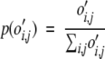(4)

(5)

(6)

In this manner, log-odds scores were calculated from the number of occurrences of the intrachain, C, interchain, T, sequential helix, S and nonsequential helix, N classes of residue contact.

Interaction entropy

Relative entropy is used as a measure of how much information one distribution of data conveys over another. If the estimated probabilities of pairwise interactions are compared to the probabilities of the null hypothesis (where the probability is dependent only upon the overall abundances of the amino acids), the relative entropy, H, is an indicator of how random the observed interactions are. H is always greater than or equal to zero. If the estimated pairwise probabilities are very close to the random distribution the relative entropy will be near zero. The larger H, the more relative information in the two distributions, and the more non-random or ordered the data. The observed probability of an i–j interaction, p(o′_i,j) is calculated as in equation 4. The random probability of an i–j interaction, p(o′_io′_j) is calculated thus:

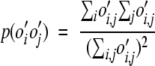(7)

The relative entropy, H between the values of p(o′_i,j) and p(o′_io′_j) is then determined.

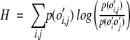(8)

The entropy relative to a random hypothesis was calculated for the distribution of pairwise amino acid contacts in the C and T classes and for the instances of S and L classes defined according to threshold loop length.

Results

Amino acid composition

The component amino acids involved in four types of transmembrane interactions were analyzed in detail (see figure in the electronic supplement). The total number of transmembrane residues studies was 2742 (an average of 16 residues per helix). Of these there were 1698 with intrachain contacts, 485 with interchain contacts, 203 with cofactor contacts, and 1633 lipid-exposed residues. There were 158 residues that were in both inter- and intrasubunit contact classes. The compositions of the classes are broadly similar. However, there are some distinct differences for particular amino acids in certain classes. The most noticeable of these are in the cofactor contacting residues. Here, glutamate, glutamine, histidine, and tryptophan are all particularly abundant, whereas there is a lack of leucine and isoleucine compared to the other residue classes. The lipid and inter-chain (oligomer) interfaces, T, are the most similar of the classes, and when compared to the intrachain, C and cofactor contacts, these surfaces are enriched in leucine, but relatively depleted in glycine, methionine, and serine. Overall, the composition of the residues in these environments reflects the need for hydrophobic residues in a transmembrane bilayer.

Pairwise interactions

Packing density

Of amino acids within the structural database, the 1698 intrasubunit contacting residues, C give rise to 4266 distinct interactions (between themselves), and each residue contacts an average of 2.51 other residues. The 485 intersubunit residues, T produce 994 pairwise interactions with each touching an average of 2.05 other residues.

For contacts within subunits the residues have more helix-helix interactions. However, this difference can be attributed to the geometry of helix packing. When a helix is in the center of a bundle, its residues are well surrounded by other residues of the same class and the number of interactions is maximized. When a helix is at the periphery of a bundle, residues can also participate in interactions with the bilayer. For the structures studied, the proportions of lipid-accessible residues in the C and T classes are 46.4% and 59.6%, respectively. Thus, the differences in interaction density reflect that intrachain contacts are, on average, more isolated from the lipid bilayer than interchain interfaces.

Contact matrices

The occurrence of amino acid pair interactions in the database and their expected counts, given a random hypothesis, was analyzed (see figure in electronic supplement). It can be seen that in many instances the random expectation is a good predictor of the observed occurrences (e.g., most Phe interactions in the C class). However, there are particular amino acid pairs for which the observed count is significantly different from the expectation (e.g., Phe-Phe in the C class). With the raw data the significance of the counts for the most abundant transmembrane residues can be demonstrated, but it is difficult to gauge the overall pattern of how well the random expectation matches the observations. Thus, the data are further presented as color density plots and as a log-odds score that compares the observed with the random expectation.

Figure 2 ▶ shows the distribution of pairwise amino acid interactions between helices in the C (within the same chain) and T (between different chains) classes. Broadly, the number of interactions of a given type reflects the abundance of the amino acid residues involved. This explains much of the differences between the two classes, for example where interactions within chains have a larger complement of hydrophilic residues. In order to determine the relative propensity of each type of interaction, the observed number of interactions has been compared with the number expected from abundance alone. These propensities, represented by a log-odds bias score, are presented in Figure 3 ▶.

Figure 2.

The relative abundance of the different pairwise interactions between residues from different transmembrane helices.

Figure 3.

(Upper panels) Log-odds scores for the estimated probability of the pairwise interactions compared to a random distribution for the C contacts within transmembrane chains and the T contacts, between transmembrane chains. The pink/red elements (negative log-odds score) represent interactions that are less abundant than expected. The blue elements (positive log-odds scores) represent interactions that are more abundant than expected. (Lower panels) Same as upper panels but calculated for the estimated probability of the pairwise interactions compared to a random distribution for the S contacts, for helices that are sequential neighbors, and the N contacts, between residues from nonsequential helices.

By looking at the log-odds scores for the two classes of helix contacts in Figure 3 ▶, particular patterns of pairwise interactions are evident for both the interchain T and intra-chain C contacts. Both classes have good a representation of the abundant hydrophobic residues, but the statistics cannot show any significant trends for the rarer hydrophilic transmembrane residues. Often overabundance of particular hydrophilic pairs can be attributed to single instances in the database.

For the most abundant transmembrane residues, interactions with a notably different log-odds bias score in the C and T classes of interactions are numerous. For example, within chains alanine disfavors isoleucine and valine contacts and favors glycine, but between chains alanine is relatively indifferent to these residues. Individual biases aside, the C and T classes show a difference in spread of log-odds scores: Between chains the abundance-derived, random hypothesis is a better model for the data for most pairs (where the log-odds scores are generally closer to zero), but there are a few abundant pairs (Ile-Ile, Val-Val, and Ala-Ala) that have a much greater log-odds bias score than the rest.

Entropy

The calculation of contacting amino acid pair entropy provides a value for the randomness of a given class of interaction as a whole. For the intrachain, C class of interactions the entropy relative to the null distribution (where the probability of an interaction depends only upon the abundances of the two independent residues) was measured to be 0.00514. For the interchain contact, T class the relative entropy was 0.01293. These values indicate that the C class of interaction on the whole is more random than the T class. The individual pair log-odds scores (Fig. 3 ▶) show that although more of the pairs in the T class have a score close to zero, the dominant contribution to the entropy calculation, and hence the origin of the order in the T class, comes from only a few hyperabundant pairs.

Sequentially neighboring helices

The composition of the S and N contacts surfaces, created by dissecting the C contacts according to helix neighbors, is very similar (see figure in electronic supplement). The sequential contact data set, S, represents 1239 residues and the nonsequential set, N, 760 residues. Given the similar composition, the differences in contact log-odds bias can be confidently attributed to differences in distribution for all residues.

The entropy associated with the comparison of pairwise interactions to a random distribution shows that the amino acid contacts are more ordered for nonsequential helices than sequential helices. For the S class the entropy is 0.00691, and for the N class the entropy is 0.01059. In this respect the nonsequential helix contacts, N are like the T contacts (oligomer interfaces). The amino acid contact log odds scores (Fig. 3 ▶) for the S and N classes show that for each situation there are different amino acid pairs with distinct biases in abundance. Although there are similarities, many pairings of the abundant transmembrane amino acids have contrasting propensities. A good example of this is that the abundant Gly-Gly pairs in the S class are not seen in the N class.

Discussion

Within and between subunits

Overall, the analyses presented here show that there are different environments within α-helical transmembrane domains. Even though these environments are similar in amino acid composition, the distribution of interactions is different in each instance.

The most distinct environment in terms of amino acid composition are the cofactor contacting residues. Here, the abundance of hydrophilic residues shows that the usual complement of transmembrane residues must be supplemented by specific rare transmembrane amino acids to create the biological function of the protein. However, these are seen here as a functional requirement rather than a structural one, as the hydrophilics are not present at oligomer interfaces. Also of note for the hydrophobic-hydrophilic distribution is the similarity of lipid and interchain abundances. Given these observations, the interchain contacts should not be included in a hydrophobic analysis of transmembrane helix organization, for example by calculating a ‘hydrophobic moment’ (Eisenberg et al. 1982).

It is beyond the scope of the statistical analyses presented here to investigate the precise context of the distinctly over-abundant and underabundant pairings. However, the fact that they exist and are significant shows that the rules that govern the association of helices within a transmembrane environment differ according to the way in which the helices are tethered to one another, or not, as the case may be. These results tend to suggest that the reason for these different rules in different situations is a result of differing thermodynamics and mechanism of protein folding.

In the analysis of contacting amino acid pairs, it has been shown that oligomer interfaces have many paired residues that are close to the random expectation, with the exception of a few highly biased pairs. The data also show that oligomer interfaces are like the lipid-facing surfaces in terms of overall composition. Thus, it seems that these interfaces generally possess an undiscerning complement of typical transmembrane residues but possess a few specific residues to mediate the structural complementarity between the two sides of the oligomer interface.

Dissecting transmembrane subunits according to the sequential relationship of interacting helices illustrates that there are different rules to amino acid selection in sequential and nonsequential situations. This is shown by both the entropy of interacting pairs compared to a random distribution and individual pair log-odds biases. As helices within transmembrane domains are almost always in contact with their sequence neighbors (Bowie 1997), such sequential neighbors appear to have a restricted choice of interacting partners. This is especially apparent when considering helices connected by short nonhelical loops. Thus, the results presented here show that the constraints imposed by the extramembranous elements upon sequentially adjacent helices affect the choice of interface residues and hence indicate a difference in the role of transmembrane helix-helix interactions in the two situations.

Folding mechanisms

With knowledge of different classes of helix-helix interactions at hand, it is possible to expand upon the two-stage model of protein folding and oligomerization (Popot and Engelman 1990). As a thermodynamic model it helps to explain the stability of the transmembrane domain, but it is evident that it can be extended to include more of the mechanistic events of membrane domain folding and oligomerization of polytopic transmembrane proteins.

Stage one

Based on several sources of evidence, stage one, the independent folding of transmembrane α-helices, no longer seems to be appropriate in every instance. The observation here of helices that obey different rules of association according to how they are connected to one another suggests that the independence or otherwise of folding is important:

1. Only five of seven transmembrane helices from bacteriorhodopsin are stable membrane helices in isolation (Hunt et al. 1997).

2. There is evidence to suggest that the α-helices have not folded completely before the helices associate laterally, within the plane of the lipid bilayer. Riley et al. (1997) showed, using CD spectroscopy on bacteriorhodopsin, that after initial domain folding there is a period of slow α-helix formation. Although this system involved spontaneous refolding (bacteriorhodopsin is peculiar in its ability to do this when substituting a detergent environment for a lipid one), the study does illustrate that the formation of all of a domain’s final α-helical content is not necessary for the initial stages of helix-helix association.

3. It was shown by von Heijne and coworkers (Mothes et al. 1997) that hydrophobic α-helices may insert into the translocon apparatus in an unfolded state. If, as suggested in some studies (Borel and Simon 1996), more than one helix can be present within the translocon machinery, when the polypeptide folds into an α-helix it will not be independent of other helices or the translocon machinery.

4. Identification of very short loops between helices makes it difficult to imagine that individual helices are truly isolated from their sequence neighbors, consistent with studies which identify the presence of multiple helices within the translocon pore (Mothes et al. 1997). It could be argued that at no stage during its initial folding is an α-helix independent and surrounded by lipid.

From the points raised here, a question is raised as to why helices in the middle of large transmembrane domains (e.g., in cytochrome c oxidase) need to be hydrophobic, if not to ensure their independent membrane stability. However, it is this hydrophobic stability which leads to a notable observation. Transmembrane helices are very stable, given a typical oil to water transfer ΔG of −42 kcal mole⁻¹. This corresponds to a much greater hydrophobicity than is required to simply anchor a helix in a membrane. The ‘extra’ hydrophobicity, if not for ensuring isolated stability, may be a requirement of the stop-transfer/translocon machinery. The rationale for the presence of such hydrophobic side chains is that the hydrophobicity of a polypeptide is much less in an unfolded state than the α-helical form, due to the presence of backbone carbonyl and amide groups. Thus, very hydrophobic side chains are consistent with the insertion of unfolded transmembrane polypeptide sections (Mothes et al. 1997); a requirement of the translocon machinery/mechanism, rather than for independent stability. The estimated free energy change for the formation of a helix from an unfolded peptide in a bilayer is in the region of −70 kcal mole⁻¹ (Engelman et al. 1986), so the observation of unfolded α-helices in the translocon apparatus (Mothes et al. 1997) is consistent with the suggestion that the translocon pore is not necessarily as hydrophobic as the lipid bilayer. This is apparent from the recent X-ray crystal structure of the translocon (Van den Berg et al. 2004).

Stage two

Stage two, the lateral association of helices to form a complete transmembrane domain, should also follow a mechanistic approach to membrane domain folding and oligomerization. First, the folding of an individual chain is distinct from the oligomerization of polypeptides. Small nonhelical loops between transmembrane α-helices will impose extremely significant constraints upon the lateral movement of helices. Thus, once membrane insertion of a polypeptide is complete, all of the transmembrane helices will be colocalized and at least partially associated.

Rapoport, von Heijne, and coworkers (Mothes et al. 1997) showed, by cross-linking experiments, that helices can contact lipids before the insertion of the next α-helix is complete, at least where the loop between helices is long (30 residues). However, this analysis also shows that the first helix is still associated with (can be cross-linked to) the translocon machinery.

The different types of transmembrane interfaces used in the analysis of residue pairings is consistent with the suggestion that the lateral association of helices has several distinct phases; multiple helices can be inserted into the Sec61 machinery, where some helices may diffuse laterally to a lipid-contactable environment before insertion has terminated and then, once fully inserted, the subunit can diffuse in the bilayer to join other polypeptides.

An in vivo model for transmembrane domain folding

We propose a consensus in vivo model for the formation of polytopic, α-helical membrane domains, which is consistent with the observations made to date and the analysis presented here (see Fig. 4 ▶).

Figure 4.

An in vivo model for the folding and oligomerization of α-helical membrane domains. See text for details.

• The transmembrane polypeptide is inserted into the trans-locon apparatus in an unfolded state.

• One or more sufficiently hydrophobic sections fold (at least partially) into α-helices which move laterally into a lipid- and translocon-contactable environment.

• Transmembrane helices associate laterally in the vicinity of the translocon apparatus until the last transmembrane segment has inserted.

• The helical bundle diffuses in the lipid bilayer until it joins other chains to form an oligomeric complex.

Several studies have tried to determine whether all of the helices of a given chain are present at the translocation machinery until insertion is complete. Transmembrane helices have been cross-linked to various parts of the translocation machinery during insertion (Do et al. 1996). Urea extraction and cross-linking to lipid molecules indicate that while insertion proceeds, helices are able to move into an at least partial lipid environment (Mothes et al. 1997). Several studies provide evidence for multiple transmembrane helices being accommodated within the translocon at a given point (Borel and Simon 1996). Although this is entirely plausible for small transmembrane domains, known domains with many membrane-spanning α-helices could not fit in the translocon pore according to the structure characterized initially by electron microscopy (Hanein et al. 1996) and more recently by X-ray crystallography (Van den Berg et al. 2004). Thus, it is beginning to seem that there is a mechanism where transmembrane helices are inserted into the translocon pore and move laterally into a partially lipid environment, forming a complete transmembrane domain as more helices accrete. Observation of the known structures (Zhou et al. 1997) illustrates that transmembrane helices almost always contact their sequence neighbors. This is consistent with the sequential addition of helices as they escape the translocon pore or a pairwise helix-helix association which forms within the translocon pore. Thus, the sequence neighbor helix interactions studied here may form at a stage of the protein folding mechanism different from that of the other interactions.

References

- Bernstein, F.C., Koetzle, T.F., Williams, G.J., Meyer Jr., E.F., Brice, M.D., Rodgers, J.R., Kennard, O, Shimanouchi, T, and Tasumi, M. 1977. The Protein Data Bank: A computer-based archival file for macromolecular structures. J. Mol. Biol. 112 535–542. [DOI] [PubMed] [Google Scholar]
- Borel, A.C. and Simon, S.M. 1996. Biogenesis of polytopic membrane proteins: Membrane segments assemble within translocation channels prior to membrane integration. Cell 85 379–389. [DOI] [PubMed] [Google Scholar]
- Bowie, J.U. 1997. Helix packing in membrane proteins. J. Mol. Biol. 272 780–789. [DOI] [PubMed] [Google Scholar]
- Chang, G., Spencer, R.H., Lee, A.T., Barclay, M.T., and Rees, D.C. 1998. Structure of the MscL homolog from Mycobacterium tuberculosis: A gated mechanosensitive ion channel. Science 282 2220–2226. [DOI] [PubMed] [Google Scholar]
- Deisenhofer, J., Epp, O., Sinning, I., and Michel, H. 1995. Crystallographic refinement at 2.3 Å resolution and refined model of the photosynthetic reaction centre from Rhodopseudomonas viridis. J. Mol. Biol. 246 429–457. [DOI] [PubMed] [Google Scholar]
- Do, H., Falcone, D., Lin, J., Andrews, D.W., and Johnson, A.E. 1996. The cotranslational integration of membrane proteins into the phospholipid bi-layer is a multistep process. Cell 85 369–378. [DOI] [PubMed] [Google Scholar]
- Doyle, D.A., Morais Cabral, J., Pfuetzner, R.A., Kuo, A., Gulbis, J.M., Cohen, S.L., Chait, B.T., and MacKinnon, R. 1998. The structure of the potassium channel: Molecular basis of K+ conduction and selectivity. Science 28069–77. [DOI] [PubMed] [Google Scholar]
- Dutzler, R., Campbell, E.B., Cadene, M., Chait, B.T., and MacKinnon, R. 2002. X-ray structure of a ClC chloride channel at 3.0 Å reveals the molecular basis of anion selectivity. Nature 415 287–294. [DOI] [PubMed] [Google Scholar]
- Eisenberg, D., Weiss, R.M., and Terwilliger, T.C. 1982. The helical hydrophobic moment: A measure of the amphiphilicity of a helix. Nature 299 371–374. [DOI] [PubMed] [Google Scholar]
- Engelman, D.M., Steitz, T.A., and Goldman, A. 1986. Identifying nonpolar transbilayer helices in amino acid sequences of membrane proteins. Annu. Rev. Biophys. Biophys. Chem. 15 321–353. [DOI] [PubMed] [Google Scholar]
- Gerstein, M. 1992. A resolution-sensitive procedure for comparing protein surfaces and its application to the comparison of antigen-combining sites. Acta Crystallogr. A 48 271–276. [Google Scholar]
- Hanein, D., Matlack, K.E., Jungnickel, B., Plath, K., Kalies, K.U., Miller, K.R., Rapoport, T.A., and Akey, C.W. 1996. Oligomeric rings of the Sec61p complex induced by ligands required for protein translocation. Cell 87 721–732. [DOI] [PubMed] [Google Scholar]
- Hubbard, T.J. and Blundell, T.L. 1987. Comparison of solvent-inaccessible cores of homologous proteins: Definitions useful for protein modelling. Protein Eng. 1 159–171. [DOI] [PubMed] [Google Scholar]
- Hunt, J.F., Earnest, T.N., Bousche, O., Kalghatgi, K., Reilly, K., Horvath, C., Rothschild, K.J., and Engelman, D.M. 1997. A biophysical study of integral membrane protein folding. Biochemistry 36 15156–15176. [DOI] [PubMed] [Google Scholar]
- Iwata, S., Lee, J.W., Okada, K., Lee, J.K., Iwata, M., Rasmussen, B., Link, T.A., Ramaswamy, S., and Jap, B.K. 1998. Complete structure of the 11-subunit bovine mitochondrial cytochrome bc1 complex. Science 281 64–71. [DOI] [PubMed] [Google Scholar]
- Jormakka, M., Tornroth, S., Byrne, B., and Iwata, S. 2002. Molecular basis of proton motive force generation: Structure of formate dehydrogenase-N. Science 295 1863–1868. [DOI] [PubMed] [Google Scholar]
- Kabsch, W. and Sander, C. 1983. Dictionary of protein secondary structure: Pattern recognition of hydrogen-bonded and geometrical features. Biopolymers 22 2577–2637. [DOI] [PubMed] [Google Scholar]
- Koepke, J., Hu, X., Muenke, C., Schulten, K., and Michel, H. 1996. The crystal structure of the light-harvesting complex II (B800–850) from Rhodospirillum molischianum. Structure 4 581–597. [DOI] [PubMed] [Google Scholar]
- Lancaster, C.R., Kroger, A., Auer, M., and Michel, H. 1999. Structure of fumarate reductase from Wolinella succinogenes at 2.2 Å resolution. Nature 402 377–385. [DOI] [PubMed] [Google Scholar]
- Locher, K.P., Lee, A.T., and Rees, D.C. 2002. The E. coli BtuCD structure: A framework for ABC transporter architecture and mechanism. Science 296 1091–1098. [DOI] [PubMed] [Google Scholar]
- Luecke, H., Schobert, B., Richter, H.T., Cartailler, J.P., and Lanyi, J.K. 1999. Structure of bacteriorhodopsin at 1.55 Å resolution. J. Mol. Biol. 291 899–911. [DOI] [PubMed] [Google Scholar]
- MacKenzie, K.R., Prestegard, J.H., and Engelman, D.M. 1997. A transmembrane helix dimer: Structure and implications. Science 276 131–133. [DOI] [PubMed] [Google Scholar]
- Mothes, W., Heinrich, S.U., Graf, R., Nilsson, I., von Heijne, G., Brunner, J., and Rapoport, T.A. 1997. Molecular mechanism of membrane protein integration into the endoplasmic reticulum. Cell 89 523–533. [DOI] [PubMed] [Google Scholar]
- Murakami, S., Nakashima, R., Yamashita, E., and Yamaguchi, A. 2002. Crystal structure of bacterial multidrug efflux transporter AcrB. Nature 419 587–593. [DOI] [PubMed] [Google Scholar]
- Nield, J., Rizkallah, P.J., Barber, J., and Chayen, N.E. 2003. The 1.45 Å three-dimensional structure of C-phycocyanin from the thermophilic cyanobacterium Synechococcus elongatus. J. Struct. Biol. 141 149–155. [DOI] [PubMed] [Google Scholar]
- Palczewski, K., Kumasaka, T., Hori, T., Behnke, C.A., Motoshima, H., Fox, B.A., Le Trong, I., Teller, D.C., Okada, T., Stenkamp, R.E., et al. 2000. Crystal structure of rhodopsin: A G protein-coupled receptor. Science 289 739–745. [DOI] [PubMed] [Google Scholar]
- Popot, J.L. and Engelman, D.M. 1990. Membrane protein folding and oligomerization: The two-stage model. Biochemistry 29 4031–4037. [DOI] [PubMed] [Google Scholar]
- Rees, D.C., DeAntonio, L., and Eisenberg, D. 1989. Hydrophobic organization of membrane proteins. Science 245 510–513. [DOI] [PubMed] [Google Scholar]
- Riley, M.L., Wallace, B.A., Flitsch, S.L., and Booth, P.J. 1997. Slow α helix formation during folding of a membrane protein. Biochemistry 36 192–196. [DOI] [PubMed] [Google Scholar]
- Royant, A., Nollert, P., Edman, K., Neutze, R., Landau, E.M., Pebay-Peyroula, E., and Navarro, J. 2001. X-ray structure of sensory rhodopsin II at 2.1-Å resolution. Proc. Natl. Acad. Sci. 98 10131–10136. [DOI] [PMC free article] [PubMed] [Google Scholar]
- Stevens, T.J. and Arkin, I.T. 2000. Do more complex organisms have a greater proportion of membrane proteins in their genomes? Proteins 39 417–420. [DOI] [PubMed] [Google Scholar]
- ———. 2001. Substitution rates in α-helical transmembrane proteins. Protein Sci. 10 2507–2517. [DOI] [PMC free article] [PubMed] [Google Scholar]
- Sui, H., Han, B.G., Lee, J.K., Walian, P., and Jap, B.K. 2001. Structural basis of water-specific transport through the AQP1 water channel. Nature 414 872–878. [DOI] [PubMed] [Google Scholar]
- Toyoshima, C., Nakasako, M., Nomura, H., and Ogawa, H. 2000. Crystal structure of the calcium pump of sarcoplasmic reticulum at 2.6 Å resolution. Nature 405 647–655. [DOI] [PubMed] [Google Scholar]
- Treutlein, H.R., Lemmon, M.A., Engelman, D.M., and Brunger, A.T. 1992. The glycophorin A transmembrane domain dimer: Sequence-specific propensity for a right-handed supercoil of helices. Biochemistry 31 12726–12732. [DOI] [PubMed] [Google Scholar]
- Tsukihara, T., Aoyama, H., Yamashita, E., Tomizaki, T., Yamaguchi, H., Shinzawa-Itoh, K., Nakashima, R., Yaono, R., and Yoshikawa, S. 1996. The whole structure of the 13-subunit oxidized cytochrome c oxidase at 2.8 Å. Science 272 1136–1144. [DOI] [PubMed] [Google Scholar]
- Van den Berg, B., Clemons Jr., W.M., Collinson, I., Modis, Y., Hartmann, E., Harrison, S.C., and Rapoport, T.A. 2004. X-ray structure of a protein-conducting channel. Nature 427 36–44. [DOI] [PubMed] [Google Scholar]
- Wouters, M.A. and Curmi, P.M. 1995. An analysis of side chain interactions and pair correlations within antiparallel β-sheets: The differences between backbone hydrogen-bonded and non-hydrogen-bonded residue pairs. Proteins 22 119–131. [DOI] [PubMed] [Google Scholar]
- Zhou, Y., Wen, J., and Bowie, J.U. 1997. A passive transmembrane helix. Nat. Struct. Biol. 4 986–990. [DOI] [PubMed] [Google Scholar]