Predicting enzyme family class in a hybridization space

Abstract

Given the sequence of a protein, how can we predict whether it is an enzyme or a non-enzyme? If it is, what enzyme family class it belongs to? Because these questions are closely relevant to the biological function of a protein and its acting object, their importance is self-evident. Particularly with the explosion of protein sequences entering into data banks and the relatively much slower progress in using biochemical experiments to determine their functions, it is highly desired to develop an automated method that can be used to give fast answers to these questions. By hybridizing the gene ontology and pseudo-amino-acid composition, we have introduced a new method that is called GO-PseAA predictor and operate it in a hybridization space. To avoid redundancy and bias, demonstrations were performed on a data set in which none of the proteins in an individual class has ≥40% sequence identity to any other. The overall success rate thus obtained by the jackknife cross-validation test in identifying enzyme and non-enzyme was 93%, and that in identifying the enzyme family was 94% for the following six main Enzyme Commission (EC) classes: (1) oxidoreductase, (2) transferase, (3) hydrolase, (4) lyase, (5) isomerase, and (6) ligase. The corresponding rates by the independent data set test were 98% and 97%, respectively.

For a newly found protein sequence, the following two questions are often asked: Is the new protein an enzyme? If it is, which enzyme family class does it belong to? Both questions are closely related to the function of the protein as well as its specificity and molecular mechanism, and hence are very important to both basic research and drug discovery practice. Although the answers can be determined by conducting various biochemical experiments, it is time-consuming and costly to do so solely by experiment approaches. Particularly, the number of sequences entering into data banks has been rapidly increasing. For instance, the number of total sequence entries in SWISS-PROT (Bairoch and Apweiler 2000) was only 3939 in 1986; it jumped to 80,000 in 1999, and recently to 155,596 according to Release 44.2 (July 30, 2004) of SWISS-PROT (http://www.expasy.org/sprot/relotes/relstat.html). With the explosion of protein sequences in data banks, it is highly desirable to develop a fast and automated method to help deal with the above two questions.

According to their Enzyme Commission (EC) numbers (Fig. 1 ▶), enzymes are mainly classified into six families (Webb 1992): (1) oxidoreductases, catalyzing oxidoreduction reactions; (2) transferases, transferring a group from one compound to another; (3) hydrolases, catalyzing the hydrolysis of various bonds; (4) lyases, cleaving C–C, C–O, C–N, and other bonds by other means than by hydrolysis or oxidation; (5) isomerases, catalyzing geometrical or structural changes within one molecule; and (6) ligases, catalyzing the joining together of two molecules coupled with the hydrolysis of a pyrophosphate bond in ATP or a similar triphosphate. Each of these families has its own subfamilies, and sub-subfamilies. In a previous study, the prediction of the subfamilies within the scope of oxidoreductases was conducted (Chou and Elrod 2003). In that study, the prediction was performed by means of the covariant discriminant function algorithm, which is a combination of the Mahalanobis distance (Mahalanobis 1936; Pillai 1985; Chou and Zhang 1994; Chou 1995) and covariance matrices (Chou and Elrod 1999b; Zhou and Assa-Munt 2001; Zhou and Doctor 2003). Although the covariant discriminant function is a very powerful algorithm, the prediction in the previous study (Chou and Elrod 2003) was based on the amino acid composition alone, and hence all the sequence-order effects were excluded. This might limit the potential for improving the prediction quality. Also, it would be logically more reasonable and practically more useful to identify a query protein according to the order of the two questions as raised at the beginning of this paper. All the subfamily predictions should be conducted after the two more basic identifications have been made. The present study was initiated in an attempt to deal with these points, introducing a new and much more powerful method to predict enzyme family class.

Figure 1.

A schematic drawing to show the six main enzyme family classes according to their EC numbers.

Materials and methods

The ENZYME database (ftp.expasy.ch) (Bairoch 2000) was used to construct the six main enzyme family classes. To avoid any bias, a redundancy cutoff operation was imposed within each class so that none of the included sequences had ≥40% identity to any other. Thus, a total of 6783 sequences were generated that consist of 1201 oxidoreductases, 2093 transferases, 2000 hydrolases, 637 lyases, 343 isomerases, and 509 ligases. Meanwhile, a total of 19,012 non-enzyme protein sequences were randomly taken from SWISS-PROT (Bairoch and Apweiler 2000) that were also subject to the same 40% redundancy cutoff operation. The accession numbers of the 6783 enzymes (classified into six classes) and the 19,012 non-enzymes are given in Supplemental Material A. Meanwhile, just for a demonstration performed later, an independent data set was also constructed as given in Supplemental Material B, in which none of the entries occurs in Supplemental Material A.

The key for improving the prediction quality of enzyme family class is to grasp the core features of a protein that are intimately related to its biological function, and then use these features to represent it. In this sense, we can use the source of the Gene Ontology (GO) Consortium (Ashburner et al. 2000) as a vehicle to formulate the prediction algorithm. The term “ontology” was originally borrowed from philosophy, where an ontology is a systematic account of existence. In other words, an ontology is an explicit specification of a conceptualization. In the GO database, gene products are organized according to the following three principles in a species-independent manner: molecular function, biological process, and cellular components.

The first two principles are directly relevant to the molecular function of an enzyme and its acting object, whereas the third one is relevant to its subcellular localization. The latter, however, is also closely associated with the function of a protein (Alberts et al. 1994; Chou and Elrod 1999a). Because the enzyme family classes are classified according to their molecular functions and acting objects (see, e.g., a monograph [Webb 1992] and Fig. 1 ▶ of a previous paper, Chou and Elrod 2003), it is anticipated that the prediction quality will be significantly improved if we use the GO database to define proteins according to the following steps.

Step 1

Mapping InterPro (Apweiler et al. 2001) entries to GO, one can get a list of data called “InterProt2GO” (ftp://ftp.ebi.ac.uk/pub/databases/interpro/interpro2go/), in which each InterPro entrance corresponds to a GO number. Because a protein may have one or more molecular functions, be used in one or more biological processes, and be associated with one or more cellular components, the relationships between InterPro and GO may be one-to-many. For instance, the InterPro entry “IPR_000003” corresponds to “GO_0003677,” “GO_0004879,” “GO_0005496,” “GO_0006355,” and “GO_0005634.” Also, because the current GO database is far from complete yet, some InterPro entrances (such as IPR_000001, IPR_000002, and IPR_000004) do not have corresponding GO numbers in the InterProt2GO list.

Step 2

The GO numbers in the InterProt2GO database are not increasing successively and in an orderly manner, and hence an operation to reorganize and compress the GO numbers thus obtained is needed. For example, after such an operation, the original GO numbers GO_0000012, GO_0000015, GO_0000030, …, GO_0046413, would become GO-compress_0000001, GO-compress_0000002, GO-compress_0000003, …, GO-compress_0001930, respectively. The database thus obtained is called the GO-compress database or the 1930D GO database, whose dimensions have been reduced to 1930 from 46,413 of the original GO database.

Step 3

Each of the 1930 GO numbers will serve as a base to define a protein P in terms of the following 1930D (dimensional) vector:

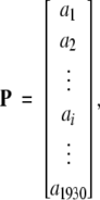(1)

where a_i = 1 if there is a hit corresponding to the i-th (i = 1, 2, …, 1930) GO number when using the program IPRSCAN (Apweiler et al. 2001) to search the InterPro functional domain database (release 6.1; Apweiler et al. 2001) for the protein P; otherwise, a_i = 0.

Step 4

If no hit, that is, no corresponding GO number, is found in the entire 1930D GO database, the protein P formulated by equation 1 will correspond to a naught vector. To cope with such a circumstance, the protein is instead defined in the (20 + λ)D PseAA (pseudo-amino-acid composition) space (Chou 2001), as given below:

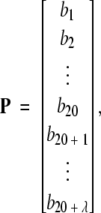(2)

where b₁, b₂, …, b₂₀ represent the 20 components of the classical amino acid composition (Chou and Zhang 1993; Zhou 1998), whereas b_{20 + 1} is the first-tier sequence-order correlation factor, b_{20 + 2} the second-tier sequence-order correlation factor, and so forth (see Appendix A). It is the additional λ components in equation 2 that incorporate some sequence-order effects into the vector representation of a protein. Generally speaking, the larger the number of the λ components, the more the sequence-order effects incorporated. However, the number λ cannot exceed the length of a protein (i.e., the number of its total residues). Also, if the number of λ is too large, the overall success rate by jackknife tests might be reduced (Chou 2001). Therefore, for different training data sets, λ may have different optimal values. For the current study, the optimal value of λ is 37. Given a protein, the (20 + 37) = 57 pseudo-amino-acid components in equation 2 can be easily derived by following the procedures as described in Chou (2001), which originally introduced the concept of pseudo-amino-acid composition. Thus, the protein that corresponds to a naught vector in the 1930D GO space (equation 1) can always be explicitly defined in the 57D PseAA space (equation 2).

The prediction was performed with the ISort (Intimate Sorting) predictor, which can be briefly described below. Suppose there are N proteins (P₁, P₂, …, P_N) that have been classified into categories 1, 2, …, μ. Now, for a query protein P, how can we predict to which category it belongs? To deal with this problem, let us define the following scale to measure the similarity between P and P_i (i= 1, 2, …, N):

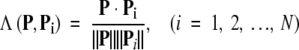(3)

where P P_i is the dot product of vectors P and P_i, and ||P|| and ||Pi|| their modulus, respectively. Obviously, when P ≡ P_i, we have Λ(P, P_i) = 1, meaning they have perfect or 100% similarity. Generally speaking, the similarity is within the range of 0 and 1, that is, 0 ≤ Λ(P, P_i) ≤ 1. Accordingly, the ISort predictor can be formulated as follows: If the similarity between P and P_k (k = 1, 2, …, or N) is the highest, that is,

(4)

where the operator Max means taking the maximum one among those in the brackets, then the query protein P is predicted to belong to the same category as P_k. If there is a tie, the query protein may not be uniquely determined, but cases like that rarely occur. The ISort predictor is particularly useful for the situation in which the distributions of the samples are unknown.

During the course of prediction, the following self-consistency principle should be followed: If a query protein could be defined in the 1930D GO space (equation 1), then the prediction should be carried out based on those proteins in the training set that could also be defined in the same 1930D GO space. If the query protein in the 1930D GO space was a naught vector and hence must be defined instead in the (20 + λ)D PseAA space (see equation 2), then the prediction should be conducted according to the principle that all the proteins in the training set should be defined in the same (20 + λ)D Pse AA space as well. Accordingly, the current ISort predictor actually consists of two subpredictors: (1) the ISort-1930D GO predictor that operates in the 1930D GO space and (2) the ISort-57D PseAA predictor that operates in the 57D PseAA space with λ = 37. The entire process is called the GO-PseAA hybridization approach.

Results and Discussion

The computation was performed in a Silicon Graphics IRIS Indigo workstation (Elan 4000). For the proteins listed in Supplemental Material A, we obtained the following results according to Steps 1–4 above:

1. Of the 6783 enzyme sequences, 6352 got the hits and hence were defined in the 1930D GO space, and the remainder were defined in the 57D PseAA space (Table 1).

2. Of the 19,012 non-enzyme proteins, 14,432 were defined in the 1930D GO space, and the remainder were defined in the 57D PseAA space.

Table 1.

Breakdown of the protein entriesa into the group defined in the 1930D GO space (eq 1) and the group in the 56D PscAA space (eq 2)

Data set	1930D GO space	57D PseAA space	Total
Enzyme	6352	431	6783
Non-enzyme	14,432	4580	19,012

^a From Supplementary Materials A.

This means that, if the definition of proteins was only based on the GO database, 6783 − 6352 = 431 proteins in the enzyme set and 19,012 − 14,432 = 4580 in the non-enzyme set would have no definition, leading to a failure of identifying their attribute. That is why it is so important to hybridize with the PseAA approach, by which not only can a protein always be defined but also its sequence-order effects may be taken into account considerably (Chou 2001). Thus, the hybrid algorithm was operated according to the following procedures: If a query protein was defined in the GO database, then the ISort-1930D GO predictor was used to predict its attribute; otherwise, the ISort-57D PseAA predictor was used to predict its attribute.

The demonstration is performed by the resubstitution test, jackknife test, and independent data set test. It is shown in Tables 2 and 3 that the overall success rates by the resubstitution test are 100% for both the case of identifying a protein sequence between enzyme and non-enzyme, and the case among the six enzyme family classes, indicating that the present method has a perfect self-consistency. However, to really examine the power of a predictor, a cross-validation procedure is needed. As is well known, the single independent data set test, subsampling test, and jackknife test are the three procedures often used for cross-validation in literature (Chou and Zhang 1995). Of these three, the jack-knife test is regarded as the most objective and effective one (Zhou and Assa-Munt 2001). A comprehensive discussion about this can be found in a review paper (Chou and Zhang 1995). Accordingly, the real power of a predictor should be measured by the success rate of the jackknife test. As shown in Tables 2 and 3, the overall jackknife success rates obtained by the current GO-PseAA hybridization approach are 93.21% for the case between enzyme and non-enzyme, and 93.58% for the case among the six enzyme family classes. Finally, as a paradigm to show how to use the present method in practical applications, the corresponding success rates performed on the independent data set of Supplemental Material B are also given in Tables 2 and 3.

Table 2.

Success rates in identifying enzyme and non-enzyme proteins

Protein attribute	Resubstitutiona	Jackknifea	Independent data setb
Enzyme	= 100%	= 93.69%	=98.00%
Non-enzyme	=100%	= 93.05%	=98.00%
Overall	=100%	= 93.21%	=98.00%

^a Using the data of Supplementary Materials A to perform resubstitution and jackknife tests.

^b Using the data of Supplementary Materials A to train the ISort-1930D GO predictor and ISort-57D PseAA predictor, and then using them to predict the independent proteins listed in Supplementary Materials B.

Table 3.

Success rates in identifying enzyme family classes

Family class	Resubstitutiona	Jackknifea	Independent data setb
Oxidoreductase	=100%	=95.92%	=100%
Transferase	= 100%	=94.12%	=97.00%
Hydrolase	= 100%	=94.80%	= 94.00%
Lyase	= 100%	=84.14%	=97.00%
Isomerase	= 100%	=84.54%	= 97.50%
Ligase	= 100%	=98.62%	=98.00%
Overall	= 100%	= 93.58%	= 97.25%

^a Using the data of Supplementary Materials A to perform resubstitution and jackknife tests.

^b Using the data of Supplementary Materials A to train the ISort-1930D GO predictor and ISort-57D PseAA predictor, and then using them to predict the independent proteins listed in Supplementary Materials B.

Conclusion

To enhance the success rate of predicting enzyme family class, the key is to catch the core features of proteins that are intimately related to their biological functions and acting objects. This can be realized by defining a protein based on the Gene Ontology (Ashburner et al. 2000) developed recently. However, the current Gene Ontology does not give a complete coverage so that some proteins cannot be meaningfully defined. Although the problem will be eventually solved as the Gene Ontology increases in size, to deal with such a situation right now, a hybrid approach was introduced by combining Gene Ontology with the pseudo-amino-acid composition (Chou 2001). With the latter, not only can a protein always be explicitly defined but also its sequence-order effects can be considerably incorporated so as to enhance the success rates as reflected in the predictions of protein subcellular location (Chou and Cai 2003b) and of protein quaternary structure (Chou and Cai 2003a). That is why a hybridization of these two approaches can yield the very high success rates in identifying non-enzyme and enzyme, as well as the enzyme family class.

With the explosion of protein sequences entering into data banks and the relatively much slower process in determining their enzymatic attributes by biochemical experiments, the current automated method may become a useful high-throughput tool for proteomics and bioinformatics.

Appendix A. The pseudo-amino-acid composition

For the convenience of readers, here we give a brief introduction to the “pseudo-amino-acid composition.” For a detailed description of it, the readers are referred to an original paper (Chou 2001).

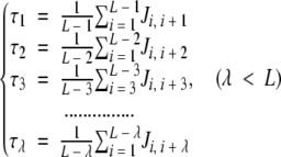
Owing to the huge number of possible sequence-order patterns, it is hard to directly incorporate the sequence-order information into a statistical prediction algorithm. Nevertheless, we can indirectly and partially take into account its effects through the following approach: Suppose a protein chain with L amino acid residues:

(A1)

where R₁ represents the residue at sequence position 1, R₂ the residue at position 2, and so forth. The sequence-order effect can be approximately reflected through a set of sequence-order-coupling factors as defined below:

(A2)

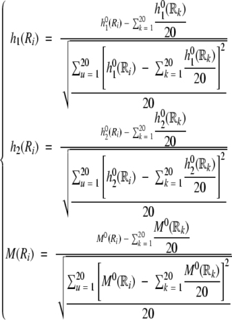
where τ₁ is called the first-tier coupling factor that reflects the sequence-order correlation between all the most contiguous residues along a protein chain (Fig. 2A ▶), τ₂ the second-tier coupling factor that reflects the sequence-order correlation between all the second-most contiguous residues (Fig. 2B ▶), τ₃ the third-tier coupling factor that reflects the sequence-order correlation between all the third-most contiguous residues (Fig. 2C ▶), and so forth. In equation A2, the coupling factor J_{i, j} is a function of amino acids R_i and R_j that is defined by the user according to the case investigated. For example, in the original paper (Chou 2001), the coupling factor is defined by:

Figure 2.

A schematic drawing to show the first-tier (A), the second-tier (B), and the third-tier (C) sequence-order correlation mode along a protein sequence. Panel A reflects the correlation mode between all the most contiguous residues; panel B, that between all the second-most contiguous residues; and panel C, that between all the third-most contiguous residues.

(A3)

where h₁(R_i), h₂(R_i), and M(R_i) are, respectively, the hydrophobicity value, hydrophilicity value, and side-chain mass of the amino acid R_i; and h₁(R_j), h₂(R_j), and M(R_j) the corresponding values for the amino acid R_j. Note that before substituting these values into equation A3, they are all subjected to a “standard conversion” as defined by the following equation:

(A4)

where we use R_i (i = 1, 2, …, 20) to represent the 20 native amino acids according to the alphabetical order of their single-letter codes: A, C, D, E, F, G, H, I, K, L, M, N, P, Q, R, S, T, V, W, and Y. The symbols h₁⁰, h₂⁰, and M⁰ represent, respectively, the original hydrophobicity value (Tanford 1962), hydrophilicity value (Hopp and Woods 1981), and the side-chain mass of the amino acid in the brackets right after the symbols. The data obtained by such a standard conversion (equation A4) will have a zero mean value and will remain unchanged if going through the same conversion procedure again. As we can see from equations A1–A4 as well as Figure 2 ▶, a considerable amount of sequence-order information has been incorporated into the λ correlation factors through the hydrophobic and hydrophilic values as well as the side-chain masses of the amino acid residues along a protein chain.

By merging the λ correlation factors into the classical amino acid composition, we obtain an augmented discrete form to represent a protein sample P:

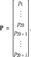(A5)

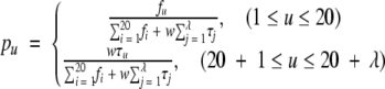(A6)

where f_i (i = 1, 2, …, 20) are the normalized occurrence frequencies of the 20 native amino acids in the protein P, τ_j the j-tier sequence-correlation factor computed according to equation A2, and w the weight factor. In the current study, we chose w = 0.05 to make the results of equation A6 within the range easier to be handled (w can, of course, be assigned other values, but this would not have a great different impact on the final results). As we can see, the first 20 numbers in equation A5 represent the classic amino acid composition, whereas the components from 20 + 1 to 20 + λ are λ correlation factors along a protein chain reflecting the effect of sequence order. A set of such 20 + λ components is called the pseudo-amino-acid composition. Using such a name is because it still has the main feature of amino-acid composition, but on the other hand, it contains information beyond the conventional amino-acid composition.

The pseudo-amino-acid composition thus defined has the following three advantages:

1. It contains more sequence-order effects not only than the 20D conventional amino acid composition (Nakashima et al. 1986), but also than the 210D pair-coupled amino-acid composition (Chou 1999) and the 400D first-order coupled amino-acid composition (Liu and Chou 1999), as reflected by a series of sequence-coupling factors with different tiers of correlation (Fig. 2 ▶; equation A2).

2. The coupling factors are defined by a combination of correlation functions that allows users to introduce any other biochemical quantities (in addition to the hydrophobicity, hydrophilicity, and side-chain mass as explicitly expressed in equation A3) to obtain the optimal results for various cases concerned.

3. The pseudo-amino-acid composition has the same formulation as the conventional one except containing more components (equation A5); accordingly, all the existing prediction algorithms based on the conventional amino acid composition can be straightforwardly extended to cover the pseudo-amino-acid composition as well.

References

- Alberts, B., Bray, D., Lewis, J., Raff, M., Roberts, K., and Watson, J.D. 1994. Molecular biology of the cell, 3rd ed., Chapter 1. Garland Publishing, New York.
- Apweiler, R., Attwood, T.K., Bairoch, A., Bateman, A., Birney, E., Biswas, M., Bucher, P., Cerutti, L., Corpet, F., Croning, M.D.R., et al. 2001. The Inter-Pro database, an integrated documentation resource for protein families, domains and functional sites. Nucleic Acids Res. 29 37–40. [DOI] [PMC free article] [PubMed] [Google Scholar]
- Ashburner, M., Ball, C.A., Blake, J.A., Botstein, D., Butler, H., Cherry, J.M., Davis, A.P., Dolinski, K., Dwight, S.S., Eppig, J.T., et al. 2000. Gene ontology: Tool for the unification of biology. The Gene Ontology Consortium. Nat. Genet. 25 25–29. [DOI] [PMC free article] [PubMed] [Google Scholar]
- Bairoch, A. 2000. The ENZYME Database in 2000. Nucleic Acids Res. 28 304–305. [DOI] [PMC free article] [PubMed] [Google Scholar]
- Bairoch, A. and Apweiler, R. 2000. The SWISS-PROT protein sequence data bank and its supplement TrEMBL. Nucleic Acids Res. 25 31–36. [DOI] [PMC free article] [PubMed] [Google Scholar]
- Chou, K.C. 1995. A novel approach to predicting protein structural classes in a (20–1)-D amino acid composition space. Proteins 21 319–344. [DOI] [PubMed] [Google Scholar]
- ———. 1999. Using pair-coupled amino acid composition to predict protein secondary structure content. J. Protein Chem. 18 473–480. [DOI] [PubMed] [Google Scholar]
- ———. 2001. Prediction of protein cellular attributes using pseudo-amino-acid-composition. Proteins 43 246–255. (Erratum 44: 60.) [DOI] [PubMed] [Google Scholar]
- Chou, K.C. and Cai, Y.D. 2003a. Predicting protein quaternary structure by pseudo amino acid composition. Proteins 53 282–289. [DOI] [PubMed] [Google Scholar]
- ———. 2003b. Prediction and classification of protein subcellular location: Sequence-order effect and pseudo amino acid composition. J. Cell. Biochem. 90 1250–1260. (Addendum 2004. 91: 1085.) [DOI] [PubMed] [Google Scholar]
- Chou, K.C. and Elrod, D.W. 1999a. Prediction of membrane protein types and subcellular locations. Proteins 34 137–153. [PubMed] [Google Scholar]
- ———. 1999b. Protein subcellular location prediction. Protein Eng. 12 107–118. [DOI] [PubMed] [Google Scholar]
- ———. 2003. Prediction of enzyme family classes. J. Proteome Res. 2 183–190. [DOI] [PubMed] [Google Scholar]
- Chou, J.J. and Zhang, C.T. 1993. A joint prediction of the folding types of 1490 human proteins from their genetic codons. J. Theor. Biol. 161 251–262. [DOI] [PubMed] [Google Scholar]
- Chou, K.C. and Zhang, C.T. 1994. Predicting protein folding types by distance functions that make allowances for amino acid interactions. J. Biol. Chem. 269 22014–22020. [PubMed] [Google Scholar]
- ———. 1995. Review: Prediction of protein structural classes. Crit. Rev. Biochem. Mol. Biol. 30 275–349. [DOI] [PubMed] [Google Scholar]
- Hopp, T.P. and Woods, K.R. 1981. Prediction of protein antigenic determinants from amino acid sequences. Proc. Natl. Acad. Sci. 78 3824–3828. [DOI] [PMC free article] [PubMed] [Google Scholar]
- Liu, W. and Chou, K.C. 1999. Protein secondary structural content prediction. Protein Eng. 12 1041–1050. [DOI] [PubMed] [Google Scholar]
- Mahalanobis, P.C. 1936. On the generalized distance in statistics. Proc. Natl. Inst. Sci. India 2 49–55. [Google Scholar]
- Nakashima, H., Nishikawa, K., and Ooi, T. 1986. The folding type of a protein is relevant to the amino acid composition. J. Biochem. 99 152–162. [DOI] [PubMed] [Google Scholar]
- Pillai, K.C.S. 1985. Mahalanobis D2. In Encyclopedia of statistical sciences (eds. S. Kotz and N.L. Johnson), pp. 176–181. John Wiley & Sons, New York.
- Tanford, C. 1962. Contribution of hydrophobic interactions to the stability of the globular conformation of proteins. J. Am. Chem. Soc. 84 4240–4274. [Google Scholar]
- Webb, E.C. 1992. Enzyme nomenclature. Academic Press, San Diego, CA.
- Zhou, G.P. 1998. An intriguing controversy over protein structural class prediction. J. Protein Chem. 17 729–738. [DOI] [PubMed] [Google Scholar]
- Zhou, G.P. and Assa-Munt, N. 2001. Some insights into protein structural class prediction. Proteins 44 57–59. [DOI] [PubMed] [Google Scholar]
- Zhou, G.P. and Doctor, K. 2003. Subcellular location prediction of apoptosis proteins. Proteins 50 44–48. [DOI] [PubMed] [Google Scholar]