Operating characteristics predicted by models for diagnostic tasks involving lesion localization

Abstract

In 1996 Swensson published an observer model that can predict receiver operating characteristic (ROC), localization ROC (LROC), free-response ROC (FROC) and alternative FROC (AFROC) curves, thereby achieving “unification” of different observer performance paradigms. More recently a model termed initial detection and candidate analysis (IDCA) has been proposed for fitting CAD generated FROC data, and recently a search model for human observer FROC data has been proposed. The purpose of this study was to derive IDCA and the search model based expressions for operating characteristics, and to compare the predictions to the Swensson model. For three out of four mammography computer aided detection (CAD) data sets all models yielded equivalent and good fits in the high-confidence region, i.e., near the lower end of the plots. The search model and IDCA tended to better fit the data in the low-confidence region, i.e., near the upper end of the plots, particularly for FROC curves for which the Swensson model predictions departed markedly from the data. For one data set none of the models yielded satisfactory fits. A unique characteristic of search model and IDCA predicted operating characteristics is that the operating point is not allowed to move continuously to the lowest confidence limit of the corresponding Swensson model curves. This prediction is actually observed in the CAD raw data and it is the primary reason for the poor FROC fits of the Swensson model in the low-confidence region.

1. INTRODUCTION

An operating characteristic summarizes observer performance in a diagnostic task. In general, an operating characteristic is a plot, as the threshold for rendering an abnormal decision is varied, of a measure of correct decisions along the y-axis vs. a measure of incorrect decisions along the x-axis. An abnormal decision for an abnormal case is termed a true positive and an abnormal decision for a normal case is a false positive. The receiver operating characteristic (ROC) ^{1, 2} is a plot of true positive fraction (TPF) vs. false positive fraction (FPF).

In the free-response localization task ^{3, 4} the observer provides mark-rating data, where a mark indicates a location that was considered suspicious, and the rating is an ordered categorization of the observer's confidence that there is a lesion at that location. The marks are classified into lesion localizations (LLs) when they are near lesions or non-lesion localization (NLs) otherwise. NLs and LLs are often loosely termed false and true positives, respectively. The free-response receiver operating characteristic (FROC) is defined ⁴ as the plot of probability of a LL vs. the mean number of NLs per image. Defining the corresponding fractions, lesion localization fraction (LLF) and non-lesion localization fraction (NLF), where it is understood that the relevant denominators for the fractions are the total number of lesions and the number of images, respectively, the FROC curve is a plot of LLF vs. NLF. In AFROC (alternative free-response receiver operating characteristic) analysis ⁵ one assigns the highest observed rating on an image as the equivalent single “ROC” rating for that image, and this is used to calculate FPF. The AFROC curve is a plot of LLF vs. FPF. In the LROC (localization ROC) paradigm the observer provides an overall rating that the image is abnormal and the marks the most suspicious region in the image ^6-9. The LROC ordinate PCL (probability of correct localization) is defined as the joint probability that a case is reported positive and the lesion is correctly localized.

Models of observer performance differ in their abilities to predict operating characteristics. The major difference occurs between ROC and all localization models because ROC models ^10-14 cannot predict any localization characteristics, but all localization models can predict ROC curves. For example, ROC models can predict ROC curves, but cannot predict LROC, FROC or AFROC curves. Models that accommodate location information and have been used in clinical studies are the FROC and AFROC models ^{5, 15}, Swensson's LROC model ⁸, the initial detection and candidate analysis (IDCA) model ¹⁶ and the search model ¹⁷. Swensson referred to as “unification” the ability of a model to predict all operating characteristics and showed how one could predict ROC, LROC, FROC and AFROC curves using his “LROC” model, henceforth termed the Swensson model. Aims of this work were to likewise unify the search model and IDCA, and to compare the abilities of these models to fit operating points for computer aided detection (CAD) data sets.

In the following we summarize IDCA and the search model and derive expressions for operating characteristics. A method for comparing the predictions of Swensson, IDCA and the search models under “matched” conditions is presented. The models were applied to mammography CAD data sets and results of these comparisons are presented. The reasons for the differing model predictions, the relationships of these models to a model of visual perception, and the rationale for using CAD data sets to evaluate models of human observer performance are discussed.

2. METHODS

2.1. The search model

According to the search model ¹⁷ the observer identifies suspicious regions in the image (decision sites) and computes a decision variable (z-sample) at each decision site. Decision sites are noise sites or signal sites depending on whether they correspond to normal regions or lesions, respectively. If a z-sample exceeds the observer's cutoff or threshold ζ the observer marks the corresponding region. Marks made because of noise site z-samples exceeding the cutoff are classified as NLs (false marks) and those made because of signal site z-samples exceeding the cutoff are LLs (true marks). The rating assigned to a mark is the bin-index of the z-sample when it is binned according to a set of ordered cutoffs. If a z-sample is less than the lowest cutoff the corresponding decision site is not marked. The z-samples for noise sites are distributed N(0,1) and z-samples from signal sites are distributed N(μ,1), where N(μ,σ²) is the normal distribution with mean μ and variance σ². The number of noise sites on an image is denoted n, where n ≥ 0, and the number of signal sites is denoted u, and 0 ≤ u ≤ S_k, where S_k is the number of lesions in the k^th image. The number of noise sites (n) is regarded as a random variable sampled from the Poisson distribution with mean λ and the number of signal sites (u) is regarded as a random variable sampled from the binomial distribution with mean S_kν. The parameters have the following interpretations: λ is the mean number of noise sites (normal regions) per image that are considered for marking; ν is the probability that a lesion is considered for marking and μ is the average difference between z-samples for lesion and noise sites. Experts are characterized by small λ, large μ and large ν (subject to the constraint that ν ≤ 1). Note that a decision site that is considered for marking is not necessarily marked: in order for the site to be marked the z-sample must exceed the lowest cutoff. An algorithm has been described to determine the parameters of the search model from FROC data ¹⁸. We will show that these estimates can be used to predict all operating characteristics.

To predict ROC curves ¹⁹ one needs two additional assumptions representing rules for assigning a single summary (“ROC-like”) rating for an image with multiple z-samples. (i) For an image with at least one mark the summary rating is the highest of all mark-specific ratings occurring on the image. (ii) For an image with no marks the observer assigns a default rating, i.e., a number smaller than the lowest allowed FROC rating, assuming higher ratings correspond to increasing confidence levels. For example, for a R-rating FROC study with allowed ratings 1, 2, …, R, the default rating could be 0. Therefore the ROC rating will range from 0 through R. The R-rating free-response study corresponds to an R+1 rating ROC study and both are described by R cutoffs and yield R operating points. [The summary ratings can be renumbered to run from 1 through R+1, which form is more familiar to users of ROC methodology, but since the ratings represent ordered categorizations, this has no effect on the analysis.] Note that an image with no marks could be due to it having one or more z-samples (n + u > 0) all of which were less than the lowest cutoff or the image yielded no z-sample (n + u = 0).

To accommodate the LROC paradigm which requires the observer to indicate a region even when n + u = 0, one assumes that for images with at least one z-sample the observer indicates the most suspicious region and a correct localization occurs if the sample is from a signal site. For images with no z-samples the observer points to a randomly chosen location and furthermore this location is never classified as a correct localization, i.e., the chance that a randomly selected location will fall close to a lesion is zero. The is similar to the assumptions made above that samples from N(0,1) or N(μ,1) exceeding the lowest cutoff are always recorded as a NLs or LLs, respectively, which preclude random misclassifications. The LROC rating assignment follows the same rules as the ROC case.

2.1.1. ROC curve

Define Φ (ζ) the probability that a sample from N(0,1) is less than ζ. Consider a normal image with at least one noise site, i.e., n > 0. The probability that the highest noise site z-sample is less than ζ is [Φ(ζ)]ⁿ whose complement is the probability that the highest noise site z-sample exceeds ζ , and this is the false positive fraction for normal images with n noise sites. To obtain FPF (ζ) for all images one performs a Poisson-weighted summation over n from 1 to ∞. The summation can be evaluated in closed form using symbolic mathematical software and the final result is Eqn. 1(a). The derivation of the true positive fraction TPF(ζ) follows a similar line of reasoning except this time one needs to consider the highest of the noise and signal site z-samples. The detailed derivation has been published ¹⁹ and the final result is Eqn. 1(b). Summarizing, the coordinates of a general point on the ROC curve are given by

$$\mathit{FPF}\left(\zeta \right)=1-e^{\left(-\frac{\lambda }{2}+\frac{1}{2}\lambda \mathit{erf}\left(\frac{\zeta }{\sqrt{2}}\right)\right)},$$ Eqn. 1(a)

$$\mathit{TPF}\left(\zeta \right)=1-{\left(1-\frac{\nu }{2}+\frac{\nu }{2}\mathit{erf}\left(\frac{\zeta -\mu }{\sqrt{2}}\right)\right)}^s{e}^{\left(-\frac{\lambda }{2}+{}^1∕_2\lambda \mathit{erf}\left(\frac{\zeta }{\sqrt{2}}\right)\right)},$$ Eqn. 1(b)

where erf is the error function ²⁰, ζ is the threshold specifying a particular operating point on the ROC curve, and s is the (constant) number of lesions per abnormal case (the extension to varying s is described in Ref. 19). It is shown in Ref. 19 that the predicted ROC curve does not continuously extend to (1,1) which is a unique and peculiar feature of the search model. This does not mean that the (1,1) point is inaccessible, rather it is not continuously accessible. Images with no decision sites are assumed to be binned in the lowest available ROC bin (0) and only when this bin is cumulated is the (1,1) point trivially - and discontinuously - reached.

2.1.2. FROC curve

The derivation of the FROC curve is particularly simple ^{18, 24}. The probability that a noise site z-sample exceeds ζ is 1−Φ(ζ). According to the Poisson assumption the mean number of noise sites per image is λ and therefore the mean number of NL marks per image at threshold ζ is λ[1−Φ(ζ)], which is the desired x-coordinate. A lesion is localized if it is considered for marking, the probability of which is ν , and if its z-sample exceeds ζ , the probability of which is 1−Φ(ζ−μ). Therefore the fraction of lesions marked at threshold ζ is ν[1−Φ(ζ−μ)], which is the desired y-coordinate. Summarizing, the coordinates of a point on the FROC curve (NLF, LLF) are given by

$$\mathit{NLF}\left(\zeta \right)=\lambda [1-\Phi \left(\zeta \right)],$$ Eqn. 2(a)

$$\mathit{LLF}\left(\zeta \right)=\nu [1-\Phi (\zeta -\mu )].$$ Eqn. 2(b)

It follows that the FROC curve starts at (0,0) and ends at (λ,ν). The x-coordinate does not extend to arbitrarily large values and the y-coordinate does not approach unity (unless ν = 1). These properties are analogous to the peculiar behavior of the ROC curve noted previously, namely the ROC curve does not continuously extend to (1,1), and is termed the finite end-point property.

2.1.3. AFROC curve

The AFROC x-coordinate is the same as the ROC x-coordinate and Eqn. 1(a) applies. The AFROC y-coordinate is identical to the FROC y-coordinate and Eqn. 2(b) applies. Since erf (−∞) = −1 the limiting coordinates of the AFROC are

$$\begin{array}{cc}\hfill \mathit{FPF}(-\infty )=& 1-e^{-\lambda }\hfill \\ \hfill \mathit{LLF}(-\infty )=& \nu ,\hfill \end{array}$$ Eqn. 3

In other words, unlike previous predictions ^{5, 8, 15}, the AFROC also exhibits the finite end-point property since it does not continuously extend to (1,1).

2.1.4. LROC curve

Swensson considered the case of more than one lesion per abnormal image, but all of the formulae in his paper ⁸ and the software implementation (LROCFIT) apply to one lesion per abnormal image. To allow comparisons this work was likewise limited to one lesion per abnormal image. The abscissa of the LROC curve is identical to that of the ROC curve and therefore Eqn. 1(a) applies. The ordinate, the probability of correct localization (PCL), can be derived using Swensson's procedure ⁸ with modifications to allow for the random n and u sampling. Considering an abnormal image with n noise-sites, a correct localization occurs if the lesion is considered for marking, the probability of which is ν and its z-sample exceeds the highest noise site z-sample on that image. The probability that the lesion z-sample z_s is less than y is

$$P(z_s<y)=\Phi (y-\mu ),$$ Eqn. 4

Therefore the probability that the lesion z-sample is in the range y to y + dy is

$$P(y<z_s\le y+\mathit{dy})=\partial \Phi (y-\mu )=\varphi (y-\mu )\mathit{dy}.$$ Eqn. 5

where ϕ is the Gaussian probability density function corresponding to N(0,1). Define A_n(y) by

$$A_n\left(y\right)\mathit{dy}\equiv \nu P(y<z_s<y+\mathit{dy})P(z_n<y),$$ Eqn. 6

where P(Z_n < y) = [Φ(y]ⁿ is the probability that z_n, the highest noise site z-sample on an abnormal image with n noise sites, is less than y. Then

$$A_n\left(y\right)\mathit{dy}\equiv \nu \varphi (y-\mu ){\left[\Phi \left(y\right)\right]}^n\mathit{dy}.$$ Eqn. 7

is the probability that the lesion is considered for marking, z_s is in the range y to y + dy, and z_n is less than y, precisely the conditions for a correct localization with confidence level in the range y to y + dy. The probability of a correct localization on an abnormal image with n noise sites for signal sites rated greater than ζ is obtained by integrating A_n(y)dy from y = ζ to y = ∞, i.e.,

$${\mathit{PCL}}_n\left(\zeta \right)={\int }_{\zeta }^{\infty }{A}_n\left(y\right)\mathit{dy}=\nu {\int }_{\zeta }^{\infty }\varphi (y-\mu ){\left[\Phi \left(y\right)\right]}^n\mathit{dy}.$$ Eqn. 8

Define Poi(n | λ) = e^−λλⁿ / n! the probability density function corresponding to a Poisson random variable with mean λ. To account for the n-sampling one performs a Poisson weighted average over all values of n, obtaining

$$\mathit{PCL}\left(\zeta \right)=\nu {\int }_{\zeta }^{\infty }\varphi (y-\mu )\left(\underset{n=0}{\overset{\infty }{\Sigma }}\mathit{Poi}(n\mid \lambda ){\left[\Phi \left(y\right)\right]}^n\right)\mathit{dy},$$ Eqn. 9

which should be compared to Eqn. 9 in Swensson's paper ⁸. Swensson's expression does not contain λ and ν but has a σ parameter (the width of the signal distribution in the Swensson model). This parameter is absent in Eqn. 9 since the signal site z-sampling in the search model has unit variance (formally σ = 1 in the search model). The random sampling of u is accounted for by the pre-factor ν and the summation over n accounts for the random number of noise sites per image.

Some understanding of how the LROC paradigm is accommodated within the framework of the search model can be obtained by considering a single rating LROC study, corresponding to a single cutoff ζ₁, where any image considered abnormal is rated “1”. From Eqn. 8 the probability of correct localization at or above confidence level ζ₁ on an abnormal image with zero noise sites (n = 0) is PCL₀(ζ₁) = ν[1 − Φ(ζ₁ − μ)]. This is seen to be the probability that a lesion is considered for marking (ν) multiplied by the probability that its z-sample exceeds ζ₁, i.e., 1 − Φ(ζ − μ). Such images will be scored as correct localizations and rated “1”. The probability that a lesion is considered for marking but its z-sample does not exceed ζ₁ is νΦ(ζ₁ − μ) and such images will be scored as correct localizations and rated “0”. Note that although the observer would not rate the image at level 1, when forced to indicate the most suspicious region the lesion will be pointed to as it is most suspicious (since the image is assumed to have no noise sites, a lesion considered for marking is automatically most suspicious). The probability that a lesion is not considered for marking is 1 − ν and such images will be classified as incorrect localizations, because the forced mark is assumed to miss the lesion (see section 2.1), and rated in bin “0” (see rating assignment rules in section 2.1). The sum of the three probabilities is unity indicating that one has accounted for all possible outcomes.

Using symbolic mathematical tools Eqn. 9 can be simplified to

$$\mathit{PCL}\left(\zeta \right)=\nu {\int }_{\zeta }^{\infty }\varphi (y-\mu )\exp \left(-\frac{\lambda }{2}+\frac{\lambda }{2}\mathit{erf}\left(\frac{y}{\sqrt{2}}\right)\right)\mathit{dy}.$$ Eqn. 10

The error function is bounded between −1 and +1 therefore the argument of the exponent is bounded between 0 and −λ and the exponent is always less than unity. An upper limit on PCL(ζ) exists, namely

$$\mathit{PCL}\left(\zeta \right)\le \nu {\int }_{\zeta }^{\infty }\varphi (y-\mu )\mathit{dy}\equiv \nu [1-\Phi (\zeta -\mu )]=\mathit{LLF}\left(\zeta \right).$$ Eqn. 11

In other words the LROC curve is always below the AFROC curve. A similar property has been noted for Swensson's model ⁸. Swensson proved two other results. (i) The area AUC_LROC under the LROC equals (2AUC_ROC − 1) where AUC_ROC is the area under the Swensson model predicted ROC curve. Empirically, this relation is also true for the search model provided one includes in the area under the LROC the area under the horizontal extension of the LROC curve from its search model predicted endpoint to FPF = 1, and AUC_ROC is the area under the search model predicted ROC ¹⁹, which includes a non horizontal extension from its end-point to (1,1). (ii) Swensson showed that the area under the AFROC equals the limiting ordinate of the LROC curve. Empirically, this also holds for the search model provided one includes a horizontal extension for the area under the search model AFROC. For the search model these relations were confirmed numerically – not analytically - for many combinations of parameters. Swensson was able to prove these relations analytically and he furthermore showed that these relations held independent of normality assumptions.

2.2. The initial detection and candidate analysis model

The initial detection and candidate analysis ¹⁶ (IDCA) model was developed for the purpose of fitting CAD FROC data. The IDCA paper does not explicitly state the sampling distributions for the numbers of noise and signal sites per image; rather it assumes Poisson and binomial distributions for the total numbers of noise sites and signal sites over the entire image set. However, Poisson and binomial sampling distributions for n and u (defined per image) are implicit in IDCA. The key difference is that unlike the search model, the IDCA method assumes, effectively, that n, the number of noise sites on an image, and u, the number of signal sites, equal the observed numbers of NL and LL marks, respectively, on the image. The search model allows for unmarked decision sites, i.e., the number of marks is ≤ the number of decision sites. Therefore IDCA effectively assumes that the lowest cutoff is negative infinity. The parameters λ and v are estimated using λ = x_end and ν = y_end, where (x_end, y_end) are the coordinates of the observed end-point of the FROC curve (see ζ → −∞ limit of Eqn. 2). In IDCA the signal distribution is N(μ, σ²) and σ² ≠ 1 is allowed. The σ parameter is absent in the search model (i.e., formally it can be regarded as fixed at unity). The parameters μ and σ are estimated by applying binormal model software, e.g., ROCFIT ²⁵, to the ratings of the NL and LL marks (i.e., the NL and LL marks are regarded as normal and abnormal “images”, respectively) and using μ = a/b and σ = 1/b, where a and b are the binormal model parameters ¹⁰ calculated by the software. The methods described in section 2.1 can be readily adapted to generate IDCA-predicted operating characteristics: (i) in sections 2.1.1 and 2.1.2 replace ζ − μ with $\frac{\zeta -\mu }{\sigma }$, and (ii) in section 2.1.4 replace y − μ with $\frac{y-\mu }{\sigma }$. The IDCA predicted FROC curve stops exactly at the observed end-point but, as discussed later, this is generally not true for other operating characteristics.

2.3. The Swensson model

Expressions for Swensson model predicted operating characteristics have been published ⁸. The model is based on the following assumptions:

1. Every image yields a highest noise z-sample and every abnormal image yields, additionally, a signal site z-sample (assuming one lesion per abnormal image).

2. The observer uses the highest z-sample (the largest of the highest noise or the signal) on an image to report the overall image rating.

3. An abnormal image is scored as a correct localization at threshold ζ if the lesion z-sample exceeds ζ and exceeds the highest noise site z-sample. Otherwise the image is scored as an incorrect localization.

4. Free-response style localizations (i.e., non-lesion and lesion localizations) occur whenever z-samples exceed ζ.

5. The highest noise z-samples are distributed N(0,1) and the lesion z-samples are distributed N(μ,σ²).

6. The highest noise and lesion z-samples are independent.

Note the distinction between correct or incorrect localizations in LROC, which are image specific definitions, and lesion or non-lesion localizations in FROC, which are region specific. The following additional assumption is needed to predict FROC curves.

• 7. Either knowledge of the total number of noise sites on an image, assumed constant, together with the assumption that the number of non-lesion localizations follows the binomial distribution, or the number of noise sites per image is infinite. In the latter case the number n_ζ of noise sites on an image with z-samples exceeding ζ follows the Poisson distribution with mean λ_ζ where λ_ζ = −ln (Φ(ζ) showing explicitly that λ_ζ → ∞ as → −∞, i.e., the number of noise sites is infinite. The Swensson model implemented in the LROCFIT software utilizes the infinite noise sites / Poisson assumption.

Assumption #1 is a key difference between the Swensson model and the search and IDCA models. It states that every image yields at least one z-sample. On a normal image the single z-sample corresponds to the highest noise (the Swensson model is not concerned with the number of individual noise site samples determining the highest noise z-sample) and on an abnormal image one has two z-samples, a highest noise and a lesion z-sample. In the search and IDCA models the number of z-samples per image is a random number (n+u) and for small λ the number of images with zero z-samples can be significant [the probability that a normal image has zero z-samples is exp(−λ) which tends to unity as λ decreases]. As noted above, the presence of images with no decision sites is what leads to the finite end-point property of search and IDCA model predicted operating characteristics. Another difference is that the search model and IDCA assume N(0,1) distributions for individual noise site z-samples, which implies non-Gaussian distribution of the highest noise ¹⁹. Swensson's model assumes an N(0,1) distribution for the highest noise.

2.4. Comparing model predictions

Since the IDCA and search models are fundamentally different from the Swensson model, it is not obvious how parameter values for the models should be matched in order to meaningfully compare the predicted operating characteristics (we assume that IDCA σ parameter is unity in which case the IDCA predicted operating characteristics are identical to the search model). The approach taken was to match the respective areas under the ROC curves and the limiting ordinates of the LROC curves. With specified values of these quantities it is possible to uniquely determine the Swensson model parameters μ_SW and σ_SW (we indicate Swensson and search model quantities with appropriate subscripts). Since the search model has three parameters, it is possible to find many combinations of parameter values yielding the targeted values for θ_SM (μ_SM, λ_SM, ν_SM) and PCL_SM (−∞). However, if one arbitrarily selects a value for λ_SM then the other two parameters can be uniquely determined.

2.5. Application to CAD data sets

Four mammography CAD data sets (A-D) were used in this work, for which we had access to the designer-level data, i.e., the z-sample (malignancy index) for all regions considered by CAD for marking. The z-samples were constrained to 0 < z < 1 and typically ranged from 0.02 to 0.98. This study used view-based analysis ¹⁸, i.e., each view with a visible mass was regarded as an abnormal “image” and the rest were regarded as normal “images”. Data set A consisted of 200 normal cases and 250 abnormal cases. The 5422 regions marked by CAD were classified by the CAD designer into 408 lesion localizations and 5014 non-lesion localizations. Data set B also consisted of 200 normal cases and 250 abnormal cases but the total number of marks was 4840. Data sets C and D consisted of 111 and 195 abnormal cases, respectively, and the total numbers of marks were 1286 and 2340, respectively, and these data sets had no normal cases. In view-based analysis these yielded 195 normal and 217 abnormal views, for data set C, and 342 normal and 380 abnormal views, for data set D. Further details on the data sets have been published ¹⁸. The raw data was binned and analyzed by the search model algorithm yielding estimates for the parameters μ_SM, λ_SM and ν_SM. The IDCA method described in section 2.2 was used to estimate μ_IDCA, λ_IDCA, ν_IDCA and σ_IDCA. The intrinsically FROC data was converted to LROC data as described previously, binned and analyzed using LROCFIT, yielding estimates for μ_SW and μ_SW.

3. RESULTS

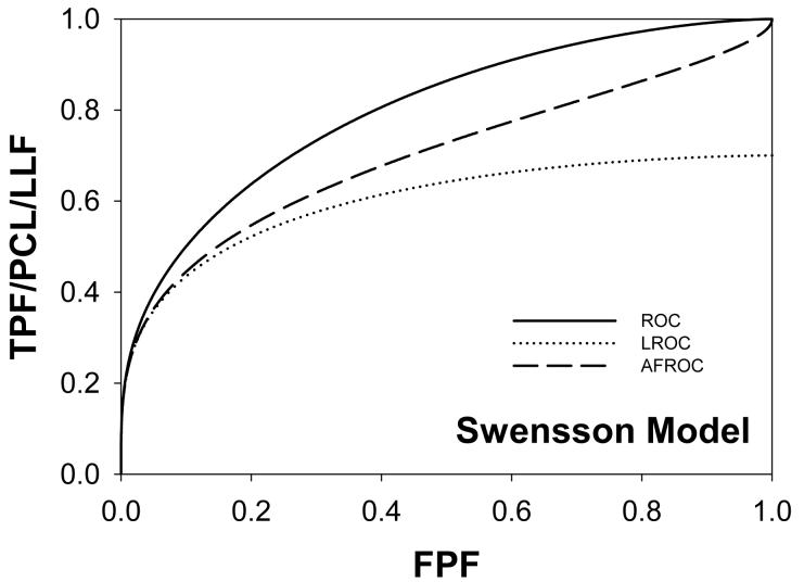
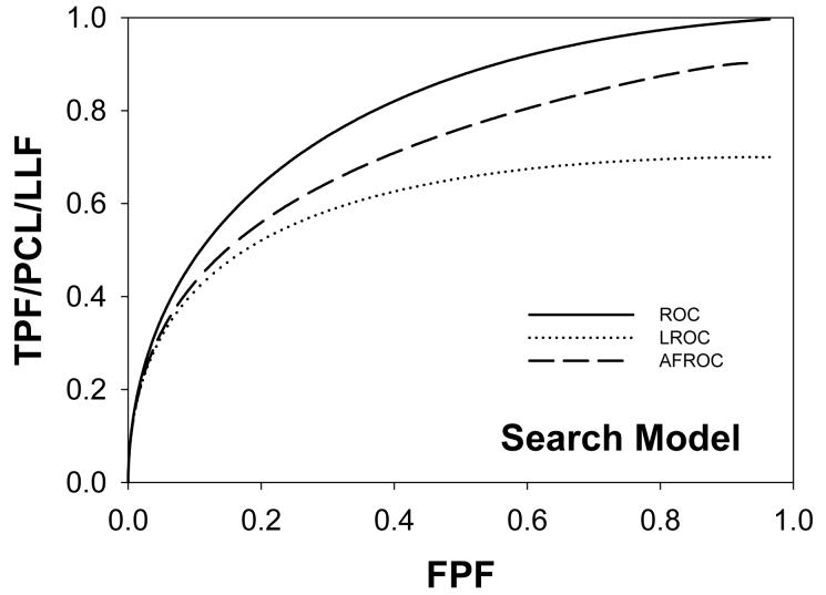
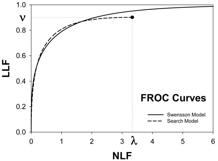
Following the procedure in section 2.4, Swensson and search model curves were generated with parameters chosen to yield areas under the ROC curves = 0.8 and limiting LROC ordinates = 0.7. Fig. 1(a) shows ROC, LROC and AFROC curves predicted by Swensson's model, Fig. 1(b) shows corresponding search model curves and Fig. 1(c) shows FROC curves (for σ_IDCA = 1, as assumed here, the IDCA predictions are identical to the search model predictions). The parameter values were μ_SW = 1.043, σ_SW = 1.719, μ_SM = 1.783, λ_SM = 3.335 and ν_SM = 0.902. The Swensson model ROC and AFROC curves extend to the upper right corner (1, 1) of the plot whereas the corresponding search model curves stop short of this point (this is most obvious for the AFROC curve). The Swensson model LROC curve abscissa extends to FPF = 1 but the search model curve does not. In either case the LROC curve is below the AFROC curve, a property of both models. In Fig. 1(c) the Swensson model FROC does not terminate inside the plotted range; in fact it extends to (∞, 1) whereas the search model curve ends at (λ_SM, ν_SM).

Figure 1.

Swensson and search model curves generated with parameters chosen to yield identical areas under the ROC curve = 0.8 and limiting LROC ordinates = 0.7. Fig. 1(a) shows ROC, LROC and AFROC curves predicted by Swensson's model, Fig. 1(b) shows corresponding search model curves and Fig. 1(c) shows FROC curves. FPF = false positive fraction, TPF = true positive fraction, PCL = probability of correct localization, NLF = non-lesion localization fraction = average # non-lesions per image, LLF = lesion localization fraction = probability that a lesion is localized. The Swensson model ROC and AFROC curves extend to the upper right corner (1, 1) whereas the corresponding search model curves do not (this is an example of the finite end-point property of all search model predicted curves). The Swensson model LROC curve abscissa extends to FPF = 1 but the search model curve does not. The Swensson model FROC does not terminate inside the plotted range, in fact it extends to (∞, 1) whereas the search model FROC curve ends inside the plotted range. For this example the IDCA predictions (not shown) are identical to the search model.

The table lists parameter values and 95% confidence intervals (in parentheses) for the Swensson, IDCA and search models for the 4 CAD data sets. The λ_IDCA, ν_IDCA parameters are identical to the abscissa and ordinate, respectively, of the end-point of the empirical FROC curve, i.e., the upper right-most operating point. The search model FROC curve end-point (λ_SM, ν_SM) is generally to the upper right of λ_IDCA, ν_IDCA. Note that the Swensson parameter μ_SW can have negative values (e.g., data set C). A similar example can be found in Table II of Swensson's paper ⁸. The search model parameter μ_SM is always positive.

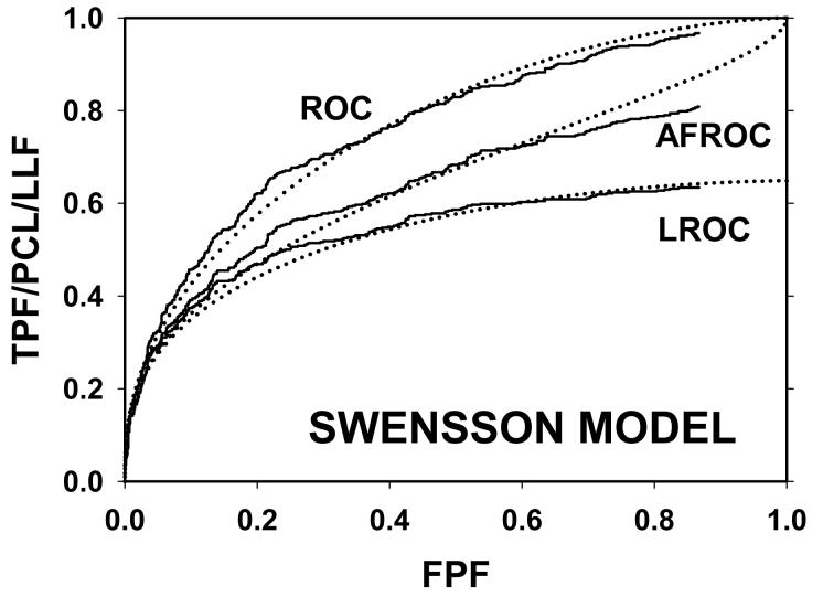
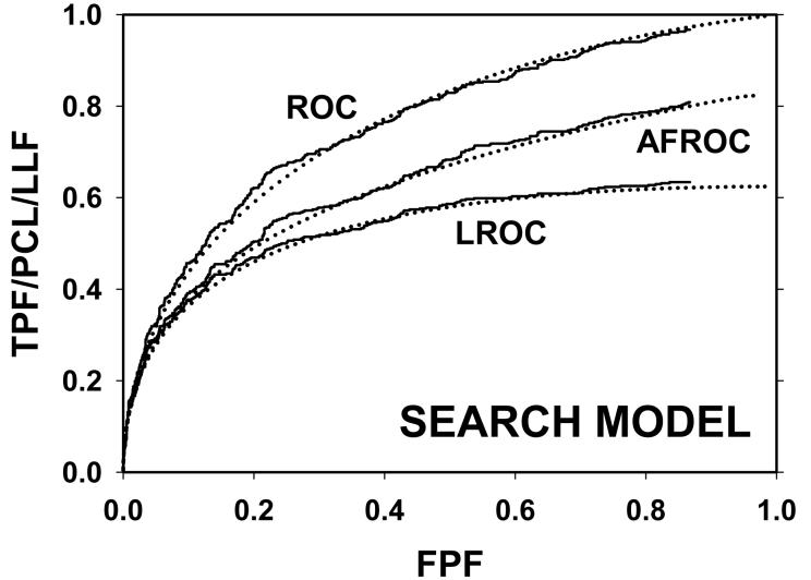
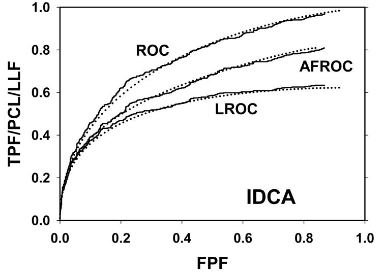
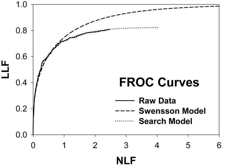
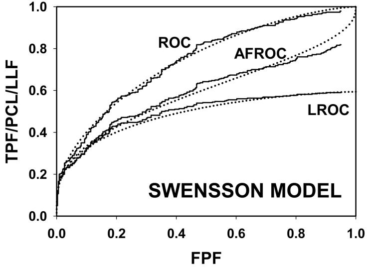
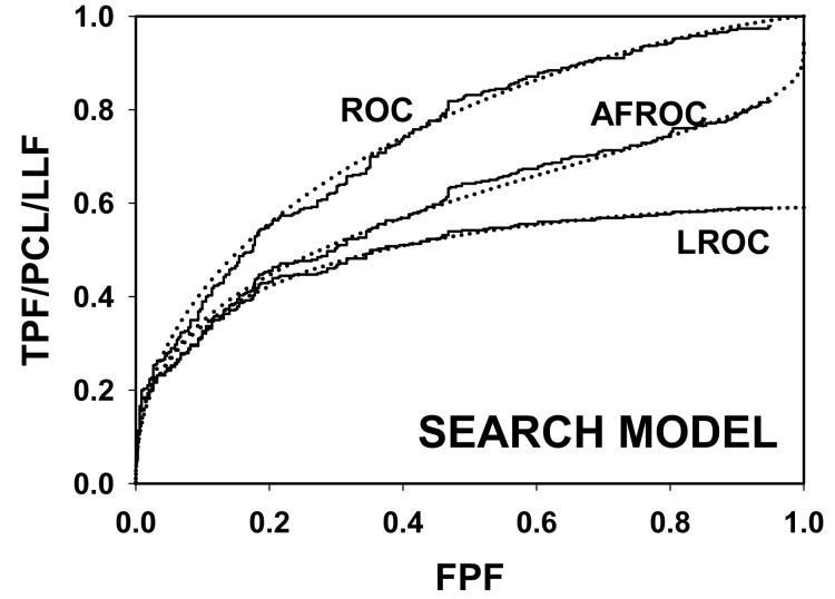
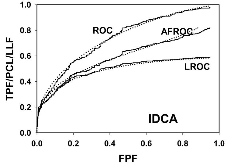
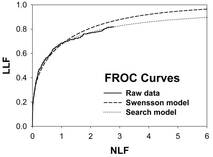
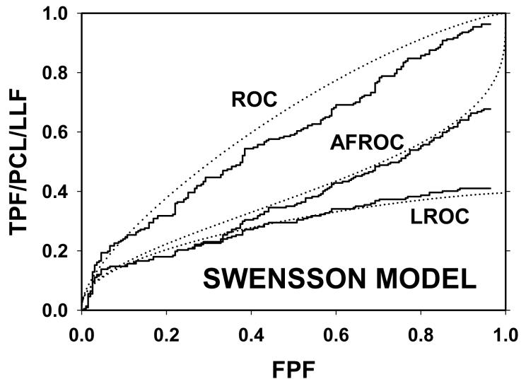
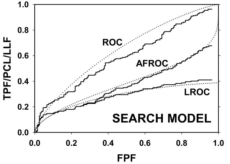
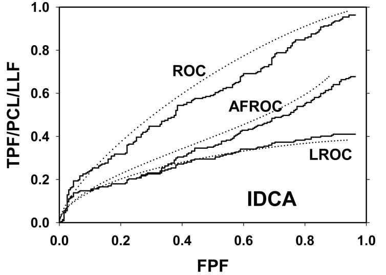
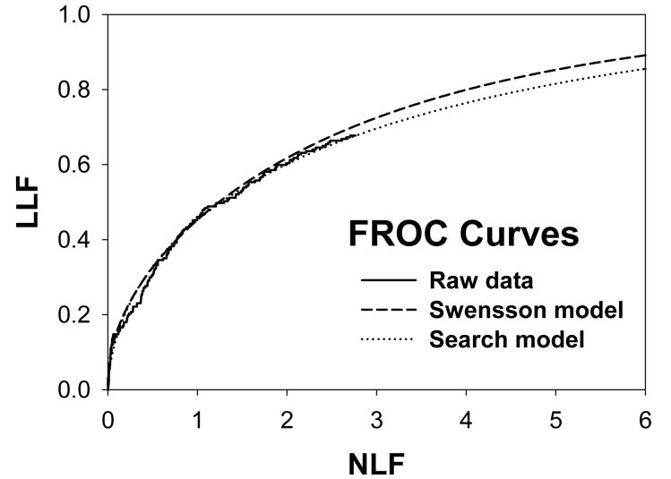
For CAD data set B, Fig. 2 (a) shows raw data (the solid curve - note that it has the “staircase” appearance characteristic of finely spaced CAD ratings) and Swensson model fitted ROC, AFROC, and LROC curves (dotted). Fig. 2 (b) shows the corresponding search model fits and Fig. 2(c) shows the IDCA fits. All models yielded reasonable fits in the lower end (high-confidence region) of the plots. IDCA and search model ROC and AFROC fits are visually better at the upper end (low-confidence region) of the plots. The finite extent of the ROC and AFROC raw data evident in this figure is inconsistent with the Swensson model fits, which extend to (1,1), but is evident in the search model and IDCA fits. Likewise the Swensson model LROC curve extends to FPF = 1 whereas the raw data, the search model and IDCA fits stop short of this value. Fig. 2 (d) shows raw data and Swensson and search model fitted FROC curves (the IDCA fit, not shown, is very close to the search model fit but it stops exactly at the observed end-point). In the high-confidence region all fits are good but in the low-confidence region (NLF > 1) the Swensson model fit deviates substantially from the data but the search model (and IDCA) yield excellent fits. As can be appreciated from this figure, the finite end-point property is most obvious for the FROC curve (d). The Swensson model fit extends to (∞,1), the raw data extends to (2.47, 0.809) which is also the end-point of the IDCA prediction, and the search model fit extends to (4.02, 0.823); see the (λ,ν) estimates listed in the table. Similar comments apply to Fig. 3 which corresponds to data set D (except the Swensson and search model ROC and AFROC yielded equivalent fits for this data set) and to data set A, not shown. For data set C, shown in Fig. 4, none of the models yielded satisfactory fits to the data, the reasons for which are unclear but possible explanations have been discussed in a prior publication ¹⁸.

Figure 2.

Comparison of the predictions for CAD data set B: (a) Swensson model ROC, AFROC, and LROC curves; (b) corresponding search model fits; (c) corresponding IDCA model fits; and (d) FROC curves predicted by the Swensson and search models (the IDCA fit, not shown, is very close to the search model fit but it stops exactly at the observed end-point). All models yielded reasonable fits in the high-confidence region of the plots. IDCA and search model ROC and AFROC fits (b and c) are slightly better in the low-confidence region of the plots. In the low-confidence region (NLF > 1) of the FROC plot the Swensson model fit deviated substantially from the data but the search model and IDCA yielded excellent fits.

Table.

Listed are parameter values and 95% confidence intervals (in parentheses) for the Swensson, IDCA and search models for the 4 CAD data sets. The λ_IDCA,ν_IDCA parameters are identical to the abscissa and ordinate, respectively, of the end-point of the empirical FROC curve [compare to Figs. 2 (d), 3 (d) and 4 (d)]. The search model FROC curve end-point (λ_SM,ν_SM) is generally to the upper right of λ_IDCA,ν_IDCA. Note that the Swensson μ- parameter μ_SW can have negative values (e.g., data set C). The corresponding search model parameter μ_SM and IDCA parameter μ_IDCA are positive.

Data Set	Parameters
	Swensson model			IDCA model			Search model
	μSW	σSW	μIDCA	λIDCA	νIDCA	σIDCA	μSM	λSM	νSM
A	0.733 (0.49, 0.98)	1.53 (1.23, 1.82)	1.66 (1.54, 1.80)	2.79 (2.71, 2.86)	0.84 (0.80, 0.87)	1.13 (1.02, 1.24)	1.95 (1.52, 2.38)	5.25 (2.79, 12.6)	0.858 (0.80, 0.92)
B	0.719 (0.55, 0.89)	1.59 (1.40, 1.78)	1.61 (1.48, 1.73)	2.47 (2.40, 2.54)	0.81 (0.77, 0.85)	1.11 (1.00, 1.22)	1.83 (1.46, 2.28)	4.02 (2.47, 9.68)	0.823 (0.77, 0.89)
C	−0.555 (−0.93, − 0.17)	1.83 (1.44, 2.22)	0.85 (0.64, 1.06)	2.76 (2.60, 2.93)	0.68 (0.61, 0.74)	1.18 (1.00, 1.35)	1.44 (0.64, 2.04)	16.81 (2.76, 40.5)	0.996 (0.61, 1.00)
D	0.497 (0.26, 0.73)	1.83 (1.55, 2.12)	1.53 (1.36, 1.71)	2.81 (2.69, 2.94)	0.82 (0.78, 0.86)	1.31 (1.16, 1.46)	2.25 (1.42, 3.09)	21.81 (3.42, 186)	0.942 (0.78, 1.00)

Figure 3.

Comparison of the predictions for CAD data set D: (a) Swensson model ROC, AFROC, and LROC curves; (b) corresponding search model fits; (c) corresponding IDCA model fits; and (d) FROC curves for Swensson and search models. These exhibit the same trends as in Fig. 2.

Figure 4.

Comparison of the predictions for CAD data set C: (a) Swensson model fitted ROC, AFROC, and LROC curves; (b) corresponding search model fits; (c) corresponding IDCA model fits; and (d) FROC curves for Swensson and search models. None of the models yielded satisfactory fits to this data set.

Swensson's software (the version we used is named “LROCFITC_NEW.EXE” and the last modification date is July 16, 1998, 2:25 PM) calculates goodness-of-fit statistics for ROC and LROC curves and the search model software calculates them for ROC and FROC curves. Therefore it is difficulty to quantitatively compare the predictions of the models, and this is the reason we refrained earlier from quoting fit statistics and simply commented on the visual impressions of the fits.

DISCUSSION

Methods for predicting all operating characteristics for the search model and IDCA have been presented. Four mammography CAD data sets were used to compare the abilities of the Swensson, search and IDCA models to fit the data. For three data sets all models yielded reasonable fits in the high-confidence region of the plots. In the low confidence region the Swensson model ROC / LROC / AFROC fits deviated somewhat from the data but the search model and IDCA yielded relatively good fits. The differences in qualities of the fits were most evident in the low confidence region of the FROC curves, where both search model and IDCA yielded excellent fits but the Swensson model failed to fit the low confidence region. For one data set none of the models yielded satisfactory fits to the data.

The search model and IDCA do not permit the operating point to move continuously to the low confidence limit of the corresponding Swensson model curves. Note the discontinuous jumps from the last ROC / AFROC raw data points in Fig. 2 to the corner (1,1). These discontinuities are predicted by the search model and IDCA but not by the Swensson model. Since CAD provides z-samples down to very low confidence levels, this is not an artifact but is intrinsic to the data. Because of the smaller λ values the finite end-point property of the search model ROC and AFROC fits is most evident in Figures 1 and 2. In Figures 3 and 4 the larger values of λ make it unlikely that an image will have no suspicious regions and the search model predicted ROC and AFROC curves approach (1,1). Since the raw data stops significantly short of this point the search model λ estimate is evidently too large and indicates that there is room for improvement in the estimation algorithm.

The IDCA publication ¹⁶ describes the prediction of FROC curves for CAD data sets. A contribution of this work is showing how to predict ROC, AFROC and LROC curves using the IDCA model. IDCA and search model FROC fits are similar except the IDCA curve stops exactly at the observed end-point whereas the search model fit generally does not. For ROC, AFROC and LROC curves the IDCA fits generally do not stop at the observed end-points [see Fig. 2(c), Fig. 3(c) and Fig. 4(c)]. This is because as long as the total numbers of NL and LL marks are preserved the empirical FROC curve, and consequently its end-point, are unaffected by the distribution of the marks between the images, but the empirical ROC, LROC and AFROC operating points, and their respective end-points, will be affected. Differences between the IDCA and search models have been discussed in more detail in earlier publications ^{17, 18}. Because it needs to account for unmarked decision sites, the search model estimation algorithm is necessarily more complex. For CAD data the simplicity of the IDCA algorithm and the excellent FROC fits make IDCA an attractive choice for fitting FROC data, but for human observers the search model prediction can be more reasonable. For example, for an observer whose uppermost operating point is on the ascending portion of the FROC curve, the IDCA fit would stop at this point, but the search model fit would predict the expected plateau of the curve.

The fact that all three models (Swensson, search and IDCA) utilize the Poisson assumption can cause confusion. In Swensson's model the Poisson λ parameter depends on the threshold ζ. Swensson's result ⁸ that λ_ζ = −ln(Φ(ζ)) shows this dependence explicitly and furthermore shows that λ_ζ → ∞ as ζ → −∞. In other words the number of noise sites per image is infinite and lowering the cutoff generates more and more NLs. In contrast, in the search model and IDCA the λ parameter is a constant, independent of ζ. This implies that the number of noise sites per image is finite and lowering the cutoff can only generate a finite number of NLs, on the average λ per image. This is why the Swensson model FROC abscissa extends to ∞ whereas the search model and IDCA curves stop at λ. Similarly, the Swensson model assumes every lesion yields a decision variable sample, which implies that at low enough threshold all lesions will be marked and LLF (ζ = −∞) = 1, but in the search model and IDCA not all lesions yield z-samples and LLF (ζ = −∞) = ν. To our knowledge Swensson's model and earlier FROC models ^{5, 15}, see below, have not been widely used in CAD FROC curve evaluation. This could be because these models having difficulty reproducing the low confidence region of the FROC curve.

Earlier FROC work ^{5, 15}, termed FROCFIT and AFROC analyses, utilized all assumptions in Section 2.3, except #3 , to predict FROC and AFROC curves. With the inclusion of assumption #3 these models can also predict ROC and LROC curves. Since the assumptions are identical, the expressions for the operating characteristics must be identical to those derived by Swensson. The difference between the approaches is how the data is collected (free-response vs. LROC) and how μ and σ are estimated. In the earlier work two procedures for estimating μ and σ were described. In FROCFIT analysis ¹⁵ μ and σ are estimated by maximizing a likelihood function determined by the NL and LL counts. In AFROC analysis ⁵ μ and σ are estimated by maximizing a likelihood function determined by the FPF and LL counts. In Swensson's method the parameters are estimated by maximizing a likelihood function determined by the FPF counts for normal images, and the overall image ratings for correct and incorrect localizations for abnormal images. Because of these differences the parameters estimated by the three methods will not, in general, be identical. But the general trends of the predictions will be similar. For example, all of these models predict that the FROC curve extends to (∞,1). The FROCFIT and AFROC methods have been applied to the data sets A - D and the fits are quite similar to those shown in Figs. 2, 3 and 4.

Several other models have been proposed for FROC curves. While detailed comparisons are outside the scope of this paper some general statements can be made. Models ^{26, 27} that assume that z-samples are obtained for all lesions (equivalent to assuming ν = 1) and the number of noise sites is sampled from a Poisson distribution with finite λ, are expected to yield fits that are intermediate between Swensson's model (and earlier FROC models) and the search model / IDCA. Specifically, for these models the FROC curve will end at (λ, 1), i.e., the x-coordinate is bounded (has a finite extent), but at low threshold all lesions are marked. If ν = 1 these models are expected to yield similar FROC fits as the search model, but as ν decreases the fits will get worse (since the data extends along the y-axis to ν, but the prediction extends to unity). A model ²⁸ that assumes that the observer performs an exhaustive search by dividing the image into lesion-sized segments and calculating a z-sample for each segment, is similar to an earlier LROC model ⁶, and both are expected to yield an FROC curve that ends at (λ′, 1) where λ′ is the image area divided by the segment area.

In our opinion the belief that observers in a clinical task perform an exhaustive search by applying equal attention units to all regions of the image, is quite prevalent in the imaging community. However, perception psychologists and other experts do not share this view. According to a model of visual perception ^29-31 the radiologist does not follow the above strategy. Rather, suspicious regions are identified during a holistic phase and in the subsequent cognitive phase decisions (to report or not to report) are made only at the regions identified during the holistic phase (these are the decision sites in the search model). This concept is explicit in the guide search model of Jeremy Wolfe ^{32, 33} and is implicit in the design of CAD algorithms ¹⁸. The perceptual model does not imply that the observer ignores some areas of the image; rather all areas are examined by the holistic mechanism but more attention units are applied to regions flagged as suspicious by the holistic mechanism. The notion that for small signals and large images the number of low confidence marks per image could be large, as required by exhaustive search models, is unsupported by any data (radiologist or CAD) that we are aware of. On the contrary, mammographers rarely mark more than a few locations per image even when they are told to mark anything suspicious no matter how low the level of suspicion (unpublished data, University of Pittsburgh). The exhaustive search view is also inconsistent with eye-movement data for mammographers where locations where the radiologist makes decisions are determined experimentally, see for example Fig. 1 in Ref. 17. Likewise, CAD algorithms calculate decision variables for a much smaller number of regions than implied by the ratio between the image area and lesion area (in fact about 12% of the images in our CAD data sets had no marks). This reflects the fact that these are expert algorithms such as could be used in the clinic. A CAD algorithm that performed lesions-sized segmentation followed by z-sampling would detect all the lesions but would pay the price of excessive false marks. In the screening mammography context the latter carries a heavy penalty in terms of unnecessary recalls and biopsies.

One may question why, if the objective is to model human observers, we chose to use CAD data to evaluate different methods of analyzing the data. The large numbers of images, the finely spaced ratings extending to very low confidence level, and the large number of marks, yield much better curve delineation and statistics than attainable with human observers and this allows one to see subtle differences in the fits. A case in point is FROCFIT analysis ¹⁵ which yielded poor FROC fits in the low confidence region (these are not shown but recall that the Swensson and earlier FROC models are identical, only the estimation procedures are different), but FROCFIT yielded excellent fits to radiologist data ¹⁵. Validating FROCFIT using only human observer data evidently yielded overly optimistic results in this case. A plausible reason is that radiologists' generally do not provide operating points that extend to very low confidence levels and in the high confidence region all models make similar predictions. CAD circumvents human observer variability, fatigue and memory effects. CAD algorithms are designed to emulate expert radiologists, and while this goal is not yet met, these algorithms are reasonable approximations to radiologists, and include the critical elements of search and localization that are central to clinical tasks. CAD algorithms involve two steps (initial detection and candidate analysis) analogous to the holistic and cognitive stages of the Kundel-Nodine visual search model ^{29, 30, 34}, which in turn is based on actual eye-tracking data. In other words CAD has a perceptual correspondence to human observers that to our knowledge is not shared by any other method of generating free-response data on clinical images. However, CAD based evaluation of observer models has its limitations. For example, CAD is unaffected by the satisfaction-of-search (SOS) phenomenon ³⁵ that is known to influence human observers. An SOS effect implies that the independence assumption, common to all models considered in this paper, may be invalid for human observers.

Operating characteristics are observables that represent different ways of quantifying performance. Given the complexity of diagnostic decision making no model is expected to be perfectly valid but the more operating characteristics a model can fit, the more confidence one should have in its validity. By this criterion the search model and IDCA appear to be closer to the truth than Swensson's model (and earlier FROC models), particularly with respect to reproducing the low confidence region of the data and the finite extent of the data. The effects of failures of the model assumptions and the arbitrary acceptance radius ³⁶ issue need to be evaluated. This study is based on a relatively small number of data sets, one of which showed unexplained behavior. Further validation with more CAD data sets is needed. Also, as noted earlier, improvement of the search model estimation algorithm is desirable.

CONCLUSIONS

Search model and IDCA based expressions for ROC, AFROC, LROC and FROC curves are derived. The predictions of the models are compared to the Swensson model. For three out of four CAD data sets all models yielded good fits in the high confidence regions of the curves, but in the low confidence regions, especially for the FROC curves, the search model and IDCA yielded superior fits. For one of the data sets none of the models yielded satisfactory fits. A unique characteristic of search model and IDCA predicted operating characteristics is that the operating point is not allowed to move continuously to the lowest confidence limit of the corresponding Swensson model curves.

REFERENCES

- 1.Metz CE. ROC Methodology in Radiologic Imaging. Investigative Radiology. 1986;21(9):720–733. doi: 10.1097/00004424-198609000-00009. [DOI] [PubMed] [Google Scholar]
- 2.Metz CE. Receiver Operating Characteristic Analysis: A Tool for the Quantitative Evaluation of Observer Performance and Imaging Systems. J Am Coll Radiol. 2006;3:413–422. doi: 10.1016/j.jacr.2006.02.021. [DOI] [PubMed] [Google Scholar]
- 3.Egan JP, Greenburg GZ, Schulman AI. Operating characteristics, signal detectability and the method of free response. J Acoust Soc. Am. 1961;33:993–1007. [Google Scholar]
- 4.Bunch PC, Hamilton JF, Sanderson GK, Simmons AH. A Free-Response Approach to the Measurement and Characterization of Radiographic-Observer Performance. J of Appl Photogr. Eng. 1978;4(4):166–171. [Google Scholar]
- 5.Chakraborty DP, Winter LHL. Free-Response Methodology: Alternate Analysis and a New Observer-Performance Experiment. Radiology. 1990;174:873–881. doi: 10.1148/radiology.174.3.2305073. [DOI] [PubMed] [Google Scholar]
- 6.Starr SJ, Metz CE, Lusted LB, Goodenough DJ. Visual detection and localization of radiographic images. Radiology. 1975;116:533–538. doi: 10.1148/116.3.533. [DOI] [PubMed] [Google Scholar]
- 7.Starr SJ, Metz CE, Lusted LB. Comments on generalization of Receiver Operating Characteristic analysis to detection and localization tasks. Phys. Med. Biol. 1977;22:376–379. doi: 10.1088/0031-9155/22/2/020. [DOI] [PubMed] [Google Scholar]
- 8.Swensson RG. Unified measurement of observer performance in detecting and localizing target objects on images. Med. Phys. 1996;23(10):1709–1725. doi: 10.1118/1.597758. [DOI] [PubMed] [Google Scholar]
- 9.Swensson RG, Judy PF. Detection of noisy visual targets: Models for the effects of spatial uncertainty and signal-to-noise ratio. Perception & Psychophyics. 1981;29(6):521–534. doi: 10.3758/bf03207369. [DOI] [PubMed] [Google Scholar]
- 10.Dorfman DD, Alf E. Maximum likelihood estimation of parameters of signal-detection theory and determination of confidence intervals - rating method data. J. Math. Psychol. 1969;6:487–496. [Google Scholar]
- 11.Dorfman DD, Berbaum KS. A contaminated binormal model for ROC data: Part II. A formal model. Acad Radiol. 2000;7(6):427–437. doi: 10.1016/s1076-6332(00)80383-9. [DOI] [PubMed] [Google Scholar]
- 12.Dorfman DD, Berbaum KS, Metz CE, Lenth RV, Hanley JA, Abu Dagga H. Proper Receiving Operating Characteristic Analysis: The Bigamma model. Acad. Radiol. 1997;4(2):138–149. doi: 10.1016/s1076-6332(97)80013-x. [DOI] [PubMed] [Google Scholar]
- 13.Metz CE, Pan X. “Proper” Binormal ROC Curves: Theory and Maximum-Likelihood Estimation. J Math Psychol. 1999;43(1):1–33. doi: 10.1006/jmps.1998.1218. [DOI] [PubMed] [Google Scholar]
- 14.Pan X, Metz CE. The “proper” binormal model: parametric receiver operating characteristic curve estimation with degenerate data. Academic Radiology. 1997;4(5):380–389. doi: 10.1016/s1076-6332(97)80121-3. [DOI] [PubMed] [Google Scholar]
- 15.Chakraborty DP. Maximum Likelihood analysis of free-response receiver operating characteristic (FROC) data. Med. Phys. 1989;16(4):561–568. doi: 10.1118/1.596358. [DOI] [PubMed] [Google Scholar]
- 16.Edwards DC, Kupinski MA, Metz CE, Nishikawa RM. Maximum likelihood fitting of FROC curves under an initial-detection-and-candidate-analysis model. Med Phys. 2002;29(12):2861–2870. doi: 10.1118/1.1524631. [DOI] [PubMed] [Google Scholar]
- 17.Chakraborty DP. A search model and figure of merit for observer data acquired according to the free-response paradigm. Phys. Med. Biol. 2006;51:3449–3462. doi: 10.1088/0031-9155/51/14/012. [DOI] [PMC free article] [PubMed] [Google Scholar]
- 18.Yoon HJ, Zheng B, Sahiner B, Chakraborty DP. Evaluating computer-aided detection algorithms. Medical Physics. 2007;34(6):2024–2038. doi: 10.1118/1.2736289. [DOI] [PMC free article] [PubMed] [Google Scholar]
- 19.Chakraborty DP. ROC Curves predicted by a model of visual search. Phys. Med. Biol. 2006;51:3463–3482. doi: 10.1088/0031-9155/51/14/013. [DOI] [PMC free article] [PubMed] [Google Scholar]
- 20.Press WH, Flannery BP, Teukolsky SA, Vetterling WT. Numerical Recipes in C: The Art of Scientific Computing. Cambridge University Press; Cambridge: 1988. [Google Scholar]
- 21.Dorfman DD, Berbaum KS, Brandser EA. A contaminated binormal model for ROC data: Part I. Some interesting examples of binormal degeneracy. Acad Radiol. 2000;7(6):420–426. doi: 10.1016/s1076-6332(00)80382-7. [DOI] [PubMed] [Google Scholar]
- 22.Pesce LL, Metz CE. Reliable and Computationally Efficient Maximum-Likelihood Estimation of “Proper” Binormal ROC Curves. Academic Radiology. 2007;14(7):814–829. doi: 10.1016/j.acra.2007.03.012. [DOI] [PMC free article] [PubMed] [Google Scholar]
- 23.Metz CE, Herman B, Shen J-H. Maximum-Likelihood Estimation of Receiver Operating Characteristic (ROC) Curves from Continuously-Distributed Data. Statistics in Medicine. 1998;17:1033–1053. doi: 10.1002/(sici)1097-0258(19980515)17:9<1033::aid-sim784>3.0.co;2-z. [DOI] [PubMed] [Google Scholar]
- 24.Chakraborty DP. FROC curves using a model of visual search. Proc. SPIE Medical Imaging: Image Perception, Observer Performance, and Technology Assessment. 2007;6515 [Google Scholar]
- 25.Metz CE. 2006 http://xray.bsd.uchicago.edu/krl/roc_soft6.htm.
- 26.Irvine JM. Assessing target search performance: the free-response operator characteristic model. Opt. Eng. 2004;43(12):2926–2934. [Google Scholar]
- 27.Hutchinson TP. Free-response operator characteristic models for visual search. Phys. Med. Biol. 2007;52:L1–L3. doi: 10.1088/0031-9155/52/10/L01. [DOI] [PubMed] [Google Scholar]
- 28.Popescu LM, Lewitt RM. Small nodule detectability evaluation using a generalized scan statistic model. Phys. Med. Biol. 2006;51(23):6225–6244. doi: 10.1088/0031-9155/51/23/020. [DOI] [PubMed] [Google Scholar]
- 29.Kundel HL, Nodine CF. A visual concept shapes image perception. Radiology. 1983;146:363–368. doi: 10.1148/radiology.146.2.6849084. [DOI] [PubMed] [Google Scholar]
- 30.Kundel HL, Nodine CF. Modeling visual search during mammogram viewing. Proc. SPIE. 2004;5372:110–115. [Google Scholar]
- 31.Kundel HL, Nodine CF, Conant EF, Weinstein SP. Holistic Component of Image Perception in Mammogram Interpretation: Gaze-tracking Study. Radiology. 2007;242(2):396–402. doi: 10.1148/radiol.2422051997. [DOI] [PubMed] [Google Scholar]
- 32.Wolfe JM. In: Attention. Pashler H, editor. University College London Press; London, UK: 1998. [Google Scholar]
- 33.Wolfe JM. Guided Search 2.0: A revised model of visual search. Psychonomic Bulletin & Review. 1994;1(2):202–238. doi: 10.3758/BF03200774. [DOI] [PubMed] [Google Scholar]
- 34.Nodine CF, Kundel HL. Using eye movements to study visual search and to improve tumor detection. RadioGraphics. 1987;7(2):1241–1250. doi: 10.1148/radiographics.7.6.3423330. [DOI] [PubMed] [Google Scholar]
- 35.Berbaum KS, Franken EA, Dorfman DD, Rooholamini SA, Kathol MH, Barloon TJ, Behlke FM, Sato Y, Lu CH, El-Khoury GY, Flickinger FW, Montgomery WJ. Satisfaction of Search in Diagnostic Radiology. Invest. Radiol. 1990;25(2):133–140. doi: 10.1097/00004424-199002000-00006. [DOI] [PubMed] [Google Scholar]
- 36.Chakraborty DP, Yoon HJ, Mello-Thoms C. Spatial Localization Accuracy of Radiologists in Free-Response studies: Inferring Perceptual FROC Curves from Mark-Rating Data. Acad Radiol. 2007;14:4–18. doi: 10.1016/j.acra.2006.10.015. [DOI] [PMC free article] [PubMed] [Google Scholar]