Robust Principal Component Analysis and Clustering Methods for Automated Classification of Tissue Response to ARFI Excitation

Abstract

We introduce a new method for automatic classification of Acoustic Radiation Force Impulse (ARFI) displacement profiles using what have been termed ‘robust’ methods for principal component analysis (PCA) and clustering. Unlike classical approaches, the robust methods are less sensitive to high variance outlier profiles and require no a priori information regarding expected tissue response to ARFI excitation. We first validate our methods using synthetic data with additive noise and/or outlier curves. Second, the robust techniques are applied to classifying ARFI displacement profiles acquired in an atherosclerotic familial hypercholesterolemic (FH) pig iliac artery in vivo. The in vivo classification results are compared to parametric ARFI images showing peak induced displacement and time to 67% recovery and to spatially correlated immunohistochemistry. Our results support that robust techniques outperform conventional PCA and clustering approaches to classification when ARFI data is inclusive of low to relatively high noise levels (up to 5dB average SNR to amplitude) but no outliers: for example, 99.53% correct for robust techniques versus 97.75% correct for the classical approach. The robust techniques also perform better than conventional approaches when ARFI data is inclusive of moderately high noise levels (10dB average SNR to amplitude) in addition to a high concentration of outlier displacement profiles (10% outlier content): for example, 99.87% correct for robust techniques versus 33.33% correct for the classical approach. This work suggests that automatic identification of tissue structures exhibiting similar displacement responses to ARFI excitation is possible, even in the context of outlier profiles. Moreover, this work represents an important first step toward automatic correlation of ARFI data to spatially matched immunohistochemistry.

Introduction

Discrimination of tissue response to transient mechanical excitation is the basis of radiation force and elastographic ultrasonic imaging methods. Rather than distinguishing tissue response by visual inspection of parametric images or time series data, we present a novel, robust approach to automated delineation of similar and dissimilar tissue displacement profiles ensuing from ARFI excitation. This technique is relevant to grouping or classifying tissue regions exhibiting consistent mechanical property.

Radiation force-based ultrasound methods have been demonstrated for delineating tissue structure via mechanical property in numerous clinically relevant applications, including discrimination of breast lesions (Soo et al. 2006; Alizad et al. 2004), myocardial RF ablations (Fahey et al. 2005a), abdominal aortic aneurysms (Mozes et al. 2005), thermally and chemically induced lesions (Bercoff et al. 2004; Fahey et al. 2004), abdominal organs (Fahey et al. 2005b), the gastrointestinal track (Palmeri et al. 2005), and thrombosis (Viola et al. 2004). Additionally, radiation force ultrasound has been shown for differentiating tissue structure in pig arteries (Zhang et al. 2006a) with confirmation by matched immunohistochemistry (Dumont et al. 2006; Behler et al. 2006) as well as in human peripheral arteries (Trahey et al. 2004; Dahl et al. 2006). In the arterial system, these techniques, along with intravascular ultrasound (IVUS) (Baldewsing et al. 2006; McKay and Shavelle 2006) and noninvasive vascular elastography (NIVE) (Maurice et al. 2005), are relevant for atherosclerosis detection and identification of plaque at risk for rupture, as well as monitoring treatment and drug therapies (Tuczo et al. 2004).

Because these imaging methods are generally reliant upon proper discrimination of incongruent tissue responses to transient mechanical excitation, visual analysis of parametric images such as depictions of Young’s moduli in elastography or tissue recovery times in Acoustic Radiation Force Impulse (ARFI) ultrasound are generally exploited. Alternatively, automated methods may be employed to further enhance differentiation of tissue responses. For example, segmentation techniques have included a fully automated statistical approach to luminal contour segmentation in intracoronary IVUS (Brusseau et al. 2004).

To appreciate the significance of classifying ARFI-induced displacement profiles, consider the physical basis of ARFI data. With peripheral arteries modeled as viscoelastic Kelvin materials, the standard linear model applies (Fung 1993):

$$f(t)+{\tau }_1\frac{df}{dt}=E\left(u(t)+{\tau }_2\frac{du}{dt}\right)$$ (1)

where f(t) is the applied ARFI force, τ₁ is the relaxation time constant for constant strain, τ₂ is the relaxation time constant for constant stress, E is the elastic modulus, and u(t) is displacement. If the ARFI pushing force is modeled to be a Heaviside function where ε is the force duration, then the displacement after time t > ε can be solved:

$$u(t)=u_o{e}^{‐\frac{t}{{\tau }_2}}$$ (2)

$$u_o=\frac{f_o}{E}\left(e^{\left(\frac{\epsilon }{{\tau }_2}\right)}‐1\right)\frac{{\tau }_2‐{\tau }_1}{{\tau }_2}$$ (3)

From equations (2) and (3), we expect typical response to ARFI excitation to exhibit an initial peak displacement (as a function of f_o, E, ε, τ₁, and τ₂) followed by an exponential recovery (a function of τ₂). Given this mathematical description for viscoelastic arterial tissue with distinct mechanical properties (E, τ₁, and, τ₂), ARFI-induced displacement profiles acquired under the same imaging parameters will be diverse in form. For instance, we expect tissue with larger Young’s modulus (E) values to demonstrate relatively smaller peak displacement in response to ARFI excitation (u_o). Likewise, we expect tissue with smaller relaxation time constant for constant stress (τ₂) to exhibit a relatively faster recovery rate. Peak displacement values from ARFI imaging are typically between 1μm and 15μm while recovery times are typically between 1ms and 5ms.

To better understand which data classification approach is suitable for discrimination of tissue response to ARFI, consider the nature and form of ARFI data (Nightingale et al. 2002). ARFI-induced axial displacements are measured over ensemble acquisition time for each of N-by-M points in the imaging field of view, where N is the number of axial samples and M is the number of lateral imaging locations interrogated in ARFI imaging. Given motion tracking over ensembles of length T, ARFI data is three-dimensional of size N-by-M-by-T, with NxM number of measured 1-by-T displacement profiles. In Figure 1, we illustrate a subset of ARFI data obtained from an in vivo familial hypercholesterolemic (FH) pig iliac artery spanning axial sample numbers 1020 to 1032 (19.62 mm to 19.85 mm), lateral location numbers 8 to 13 (−6.42 mm to −4.16 mm), and time samples 1 to 59 (0 ms to 8.12 ms). From the N-by-M-by-T matrix of ARFI data (illustrated as a 3D plot in Fig. 1a), we have access to individual displacement profiles through time T at a given N-by-M spatial location (Fig. 1b). We can also display two-dimensional ARFI images of displacement at a given time sample T (Fig. 1c), where T in this case is time sample number 10 (1.49 ms).

Fig. 1.

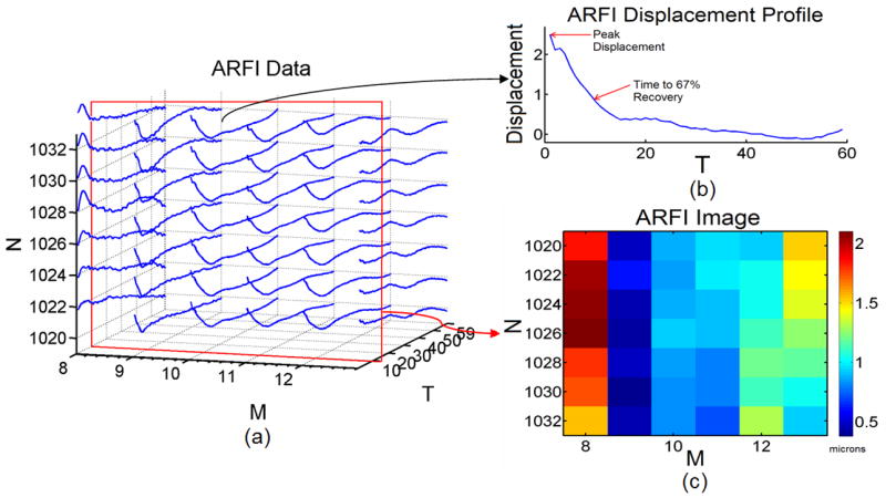
ARFI data from an in vivo FH pig iliac artery displayed in a) a 3D plot of N-by-M-by-T ARFI data. The illustration displays ARFI displacement data from axial samples 1020 to 1032, lateral image locations 8 to 13, and time samples 1 to 59. b) A single ARFI displacement profile from axial sample 1032 and lateral location 10 is displayed. Peak displacement and time to 67% recovery information is obtained (red arrows). At temporal sample number 10 from 1(a) (red box) an ARFI image c) is depicted showing displacement in microns.

Three-dimensional ARFI data can be evaluated in multiple ways to identify tissue regions exhibiting comparable responses to ARFI excitation. One approach is to assess the data parametrically, mapping the overall peak displacement or time to 67% recovery from peak displacement measured for each displacement profile to a two-dimensional (N-by-M) display. Likeness in these parameters of interest can then be recognized with orientation to spatial distributions by visual inspection of the parametric images. Another means for distinguishing tissue responses to ARFI excitation is to evaluate displacement and recovery continuously over time. This can be achieved two-dimensionally by comparing a selection of 1-by-T displacement profiles, which each represent displacement and recovery for a given point over the period of ensemble acquisition. Three-dimensionally, displacement values measured at each time point in the N-by-M field of view can be displayed as frames in a movie, which enables visual analysis of both spatial and temporal characteristics of tissue response to ARFI excitation.

Rather than visual inspection, we present a technique for automated ARFI displacement profile classification to group tissue regions with similar responses to ARFI excitation. Our method entails two primary steps: 1) robust principal component analysis (ROBPCA) is applied to ARFI displacement profiles measured in a region of interest for rank reduction, and 2) robust K-Means clustering (ROBCLUST) is applied to the derived principal component coefficients for outlier segregation and discrimination of tissue exhibiting similar response to ARFI excitation.

Materials and Methods

Robust Principal Component Analysis

Principal component analysis (PCA) and independent component analysis (ICA) are forms of blind source separation (BSS), which has previously been demonstrated in ultrasound applications for adaptive clutter rejection as well as filtering physiological and ARFI-induced tissue and blood motion (Gallippi and Trahey 2002; Gallippi et al. 2003; Gallippi and Trahey 2004). Briefly, BSS is a linear transformation used to describe series of observed data points as summations of a set of constitutive ‘sources’, or basis vectors. Unlike other linear transformations such as the Fourier transform, BSS basis vectors are derived adaptively using no a priori information about the basis vectors themselves. Instead, BSS assumes statistical relationships between the basis vectors. In the case of PCA, the basis vectors are assumed to be orthogonally distributed.

We can describe classic PCA (CPCA), then, as a linear transformation that maps the data to a new coordinate system spanned by the derived orthogonal basis vectors. The basis vectors, computed as the eigenvectors of the data’s empirical covariance matrix, describe the variance of the data through a small number of linear combinations. The greatest variance by any projection of the data comes to lie on the first coordinate (called the first principal component), the second greatest variance on the second coordinate, and so on. By projecting the data onto only a select subset of higher or lower order principal components, the dimensionality of the data set can be reduced while retaining or rejecting those characteristics of the data set that contribute most to its variance (Fukunaga 1990). In application to CPCA methods for automatic classification of ARFI-induced displacement profiles in peripheral vasculature, the ARFI data is projected onto the smallest number of higher order principal components that exceed a predetermined threshold energy level. This projection yields what are termed ‘principal component coefficients,’ which can then be clustered using conventional K-means clustering methods as described in Levy et al. (2006) and Mauldin et al. (2006). In Figure 2, a block diagram is displayed illustrating CPCA and clustering methods for ARFI-induced displacement profile classification.

Fig. 2.

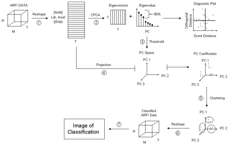
Block diagram for CPCA methods to ARFI-induced displacement profile classification.

When CPCA methods for automatic classification of ARFI-induced displacement profiles are used, variance may be dominated by what are termed ‘outlier profiles,’ which would skew the most energetic classic principal components toward anomalous observations. These outlier displacement profiles represent a measured tissue response to ARFI excitation that is not consistent with the Kelvin model for viscoelastic tissue (eqns 1, 2, and 3) and may arise in non-viscoelastic tissue or from corruption in measured response to ARFI excitation from physiological motion or other noise sources.

Rather than taking the classical approach to automatic classification, we implement robust PCA (ROBPCA) methods to obtain principal components that are not as significantly influenced by outlier observations.

ROBPCA combines two robust approaches that are termed ‘projection pursuit’ methods for initial dimensionality reduction and ‘robust covariance estimation’ methods to yield robust principal components from the lower-dimensional data. We have implemented the algorithm here using the MATLAB (MathWorks, Natick, MA, USA) code provided in Libra: a Matlab Library for Robust Analysis (Verboven and Hubert 2005). The methods of ROBPCA are very lengthy and are described in great detail in Hubert et al. (2005); we present a less involved overview of the methods here.

The ARFI-induced displacement profiles measured in our region of interest are first organized into rows to form a n by p data matrix that we will denote X_{n, p} where n is the number of displacement profiles and p is the number of original variables (time samples through ensemble acquisition in this case). Unlike CPCA, which recall computes the PC basis functions as the eigenvectors of the covariance matrix of the centered (mean reduced) data, ROBPCA first preprocesses X_{n, p} and finds its ‘least outlying’ data points (displacement profiles in this case). Based on these least outlying points, a preliminary covariance matrix, S₀, is constructed and is used to robustly estimate eigenvalues and eigenvectors. The robust center of the data, μ, is calculated by finding the mean of the least outlying data points in X_{n, p}. Subsequently, the eigenvalues (derived from S₀ ) are arranged in the form of what is termed a ‘scree plot,’ which displays monotonically decreasing eigenvalues versus associated PC. From the scree plot, we determine the point of inflection in eigenvalue magnitude. This point is associated with the kth PC, and we retain the first k principal components to span the displacement profile subspace. After determining k, ROBPCA robustly estimates what is termed the ‘robust scatter matrix’ and computes the k eigenvalues, l_1:k, and corresponding eigenvectors, which are the robust PC basis functions. The robust scatter matrix of rank k is defined as:

$$S=v_{p,k}{L}_{k,k}{v}_{p,k}^{\prime }$$ (4)

where v_p,k are the k PC basis functions arranged in columns, and L_k,k is a diagonal matrix with eigenvalues arranged in monotonically descending order l_1:k.

The robust scores are then calculated as the projection of our k PC basis functions onto the robustly centered data set:

$$T_{n,k}=(X_{n,p}‐1_n\mu )v_{p,k}$$ (5)

where 1_n is a n-by-1 column vector of ones, μ is the robust center of all ‘least outlying’ displacement profiles in X_{n, p}, and T_n,k are the robust score values. The score values describe the relative contribution of each robust PC basis function to each displacement profile. As such, each reduced dimension displacement profile can then be recovered as the sum of the robust PC basis functions weighted by the profile’s k associated robust score values. Note that robust score values are conceptually akin to PC coefficients, but the robust score values are less sensitive to outlier displacement profiles.

In addition to robustly reducing the rank of our collection of ARFI-induced displacement profiles, ROBPCA also produces an outlier diagnostic plot that is relevant to outlier rejection. The diagnostic plot is formulated by calculating the orthogonal distances from the original to the rank reduced displacement profiles; the orthogonal distance OD_i of each observation x_i is calculated

$$O{D}_i=\Vert x_i‐{\mu }^{\prime }‐v_{p,k}{t}_i^{\prime }\Vert$$ (6)

where μ′ is the robust center of all ‘least outlying’ profiles in X_{n, p} arranged as a column vector, and $t_i^{\prime }$ are the robust scores for observation i arranged as a column vector. The orthogonal distance value corresponds to the amount of variance for a given observation that is not explained by the first k principal components, or similarly, the orthogonal distance value corresponds to the distance of the observation from the RPC subspace. The robust score distance, SD_i, for each profile, i, is calculated by

$$S{D}_i=\sqrt{\sum _{j=1}^k\frac{t_{ij}^2}{l_j}}$$ (7)

where t_ij are the robust score values, k is the number of principal components, and l_j are the associated eigenvalues.

Both orthogonal and robust score distances serve to decipher outlier ARFI-induced displacement profiles in the following manner: Orthogonal distance is plotted versus score distance in the form of a ‘diagnostic plot.’ Assuming a normal distribution, a threshold is drawn for each distance such that exceeding each threshold is expected to have less than 2.5% probability. Displacement profiles associated with orthogonal and score distances above these thresholds are labeled outliers.

Utilizing the ROBPCA outlier diagnosis, observations are rejected that exceed the orthogonal and score distance thresholds. These observations are assumed to be outliers in the data set that exhibit both a large orthogonal distance to the RPC subspace and a large projection onto the RPC subspace. To accomplish this step, we implement the clustering algorithm ROBCLUST that begins by segregating anomalous observations. Next, ROBCLUST assigns these points to their own cluster group and segments the remaining and non-outlying data into a predetermined number of clusters by traditional K-means methods. Each displacement profile then has an assigned cluster number, which is spatially re-indexed back to the original ARFI data arrangement for data analysis. Figure 3 displays a block diagram illustrating ROBPCA and clustering methods for ARFI displacement profile classification.

Fig. 3.

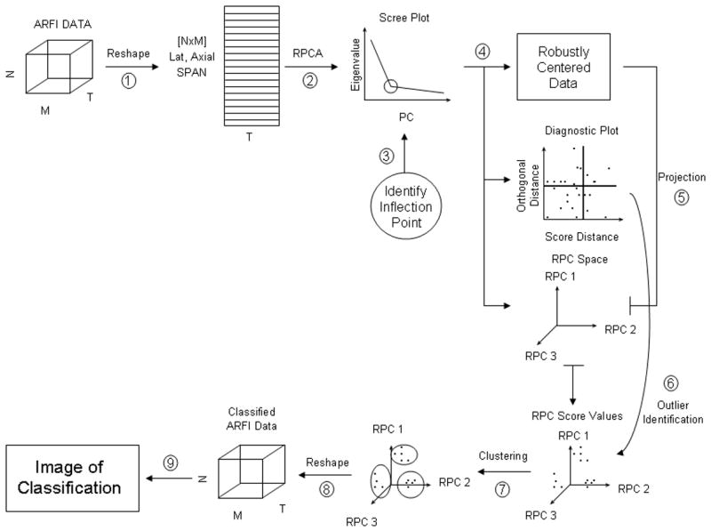
Block diagram for RPCA methods to ARFI-induced displacement profile classification.

Synthetic data set construction

Synthetic tri-layered data sets were created to simulate measured response of viscoelastic tissue to ARFI excitation, as described by equations 1, 2, and 3. Consistent with the Kelvin model for viscoelasticity, simulated curves were constructed for each synthetic layer of ‘tissue’ to mimic an exponential decay with an assigned peak displacement, u_o, and recovery rate, 1/τ₂, parameter (eqn 2). These parameters reflected the mechanical properties (E, τ₁, and τ₂) of the synthetic tissue being simulated. For instance, the assigned peak displacement for a given region of tissue was a function of E, τ₁, and τ₂ while the recovery rate was a function of τ₂ alone (eqn 3).

In order to model the presence of noise and outlier profiles in ARFI data, synthetic tissue displacement profile data sets were created for these experiments of four primary classifications: no outliers and moderate noise, no outliers and high noise, outliers and moderate noise, and outliers and high noise. Within each primary classification of synthetic tissue data set, there were three different sub-classifications of data sets (synthetic tissue data set 1 (ST 1), synthetic tissue data set 2 (ST 2), and synthetic tissue data set 3 (ST 3)) with varied peak displacement and recovery rate parameters, for a total of 12 distinct data sets. All data sets consisted of 3,000 total curves, and we used 50 time points to describe each curve so that the data sets were size 300-by-10-by-50. A summary of the assigned peak displacement, u_o, and recovery rate, 1/τ₂, parameters for each synthetic tissue layer of the 12 total synthetic tissue data sets is displayed in Table 1.

Table 1.

Summary of synthetic tissue layer displacement curve parameters for all 12 synthetic tissue data sets

	Moderate Noise						High Noise
ST 1	Outliers			No Outliers			Outliers			No Outliers
		uo	1/τ2		uo	1/τ2		uo	1/τ2		uo	1/τ2
	Layer 1	1.3	0.05	Layer 1	1.3	0.05	Layer 1	1.3	0.05	Layer 1	1.3	0.05
	Layer 2	1.0	0.2	Layer 2	1.0	0.2	Layer 2	1.0	0.2	Layer 2	1.0	0.2
	Layer 3	0.7	0.5	Layer 3	0.7	0.5	Layer 3	0.7	0.5	Layer 3	0.7	0.5
ST 2	Outliers			No Outliers			Outliers			No Outliers
		uo	1/τ2		uo	1/τ2		uo	1/τ2		uo	1/τ2
	Layer 1	1.3	0.2	Layer 1	1.3	0.2	Layer 1	1.3	0.2	Layer 1	1.3	0.2
	Layer 2	1.0	0.2	Layer 2	1.0	0.2	Layer 2	1.0	0.2	Layer 2	1.0	0.2
	Layer 3	0.7	0.2	Layer 3	0.7	0.2	Layer 3	0.7	0.2	Layer 3	0.7	0.2
ST 3	Outliers			No Outliers			Outliers			No Outliers
		uo	1/τ2		uo	1/τ2		uo	1/τ2		uo	1/τ2
	Layer 1	1.0	0.05	Layer 1	1.0	0.05	Layer 1	1.0	0.05	Layer 1	1.0	0.05
	Layer 2	1.0	0.2	Layer 2	1.0	0.2	Layer 2	1.0	0.2	Layer 2	1.0	0.2
	Layer 3	1.0	0.5	Layer 3	1.0	0.5	Layer 3	1.0	0.5	Layer 3	1.0	0.5

Synthetic tissue data sets with no outliers included three synthetic tissue layers (upper tissue, middle tissue, and lower tissue) with simulated displacement curves of varied peak displacement and recovery rates. While containing the same three synthetic tissue layers and simulated displacement curves as in the no outlier data set, the data set with outliers contained three additional synthetic tissue regions with associated outlier displacement curves so that 10% of the total data set consisted of anomalous observations. These outlier curves were selected from in vivo ARFI data acquired in an FH pig iliac artery as anomalous observations that did not display the recovery behavior typical of ARFI displacement profiles measured in arterial tissue. Recall that outlier profiles can arise in ARFI data from non-viscoelastic tissue or from corruption in measured response due to noise sources or physiological motion. In outlier contaminated data sets, each layer (upper tissue, middle tissue, and lower tissue) consisted of 900 simulated displacement curves and 100 outlier displacement curves centrally positioned within the layers. Figures 4 and 5 illustrate the synthetic data.

Fig. 4.

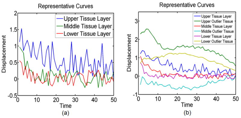
a) Representative simulated tissue displacement curves for upper tissue, middle tissue, and lower tissue layers for the no outlier, high noise, ST 1 data set, and b) representative simulated viscoelastic tissue displacement curves and simulated outlier tissue displacement curves for upper tissue, middle tissue, and lower tissue layers for the outlier, moderate noise, ST 1 data set.

Fig. 5.

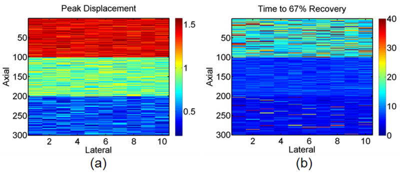
a) Peak displacement and b) time to 67% recovery images for the no outlier, high noise, ST 1 data set.

In order to model noise in synthetic tissue response to ARFI excitation, data sets classified as having high noise were assigned 0.562 peak to peak normally distributed noise to curve amplitude (representing 5dB SNR at an amplitude of 1) and 0.1 peak to peak of normally distributed noise to recovery rate. Conversely, tissue displacement data sets classified as having moderate noise contained 0.316 peak to peak normally distributed noise to curve amplitude (representing 10 dB SNR at an amplitude of 1) and 0.05 peak to peak of normally distributed noise to recovery rate. Outlier tissue displacement curves were assigned 0.1 peak to peak normally distributed noise to amplitude in both high noise and moderate noise data sets.

For sub-classification synthetic tissue data set 1 (ST 1), both peak displacement and recovery rates are varied across all three synthetic tissue layers so that the 1000 upper layer curves (in rows 1 to 100) in the tissue displacement data set were assigned peak displacements of 1.3 and recovery rates of 0.05, the middle 1000 curves (in rows 101 to 200) were assigned peak displacements of 1.0 and recovery rates of 0.2, and the bottom 1000 curves (in rows 201 to 300) were assigned peak displacements of 0.7 and recovery rates of 0.5. Representative tissue displacement curves from each of the three layers of a no outlier, high noise, ST 1 data set are displayed in Figure 4a while Figure 4b illustrates representation tissue response curves from each of six regions of an outlier, moderate noise, ST 1 data set.

Similarly synthetic tissue data set 2 (ST 2) varies in only peak displacement from 1.3, 1.0, and 0.7 across the upper, middle, and lower regions respectively while recovery rates are held constant at 0.2. In synthetic tissue data set 3 (ST 3), peak displacement is held constant at 1.0 while recovery rates are varied from 0.05, 0.2, and 0.5 across the upper tissue, middle tissue, and lower tissue layers respectively.

In order to validate the use of a ROBPCA plus ROBCLUST algorithm for optimal classification of ARFI data, we compared the method to five other possible PCA plus clustering techniques including CPCA plus K-means, ROBPCA plus K-means, CPCA plus partition around medoids (PAM), ROBPCA plus PAM, and CPCA plus ROBCLUST. Whereas K-means uses Euclidean distances to minimize sum of point-to-centroid distances (O’Rourke and Toussaint 2004), the PAM algorithm minimizes the dissimilarity matrix and is therefore more robust to outliers than K-means. A medoid is defined as the most centrally located point within a given cluster where the average dissimilarity between the medoid and other points within the cluster are minimized. We have used the PAM algorithm as implemented on MATLAB through code obtained from Libra: a Matlab Library for Robust Analysis which is described in detail in (Kaufman and Rousseeuw 1990).

In synthetic tissue data sets without outliers, a correct classification result was defined as three separate classifications corresponding to the upper tissue, middle tissue, and lower tissue layers. Similarly, for the synthetic tissue data sets with outliers, a correct classification result was defined as three distinct classifications for upper tissue, middle tissue, and lower tissue layers and one distinct classification for the remaining regions of synthetic outlier tissue. Our percent correct value from the classification result was then calculated as the ratio of observations in the correct classification to the total number of observations (3,000 curves).

An important consideration in evaluation of a novel classification method is how to validate results and compare performance against alternative approaches. We have elected to assess the effectiveness of various segmentation methods by calculating 2 measures: percent correct (described above) and average silhouette value. Following robust score clustering into n number of clusters, the silhouette value S_i for each observation was calculated by

$$S_i=\frac{min({\widehat{d}}_{i,n‐1}‐{\widehat{c}}_i)}{max({\widehat{c}}_i,min({\widehat{d}}_{i,n‐1}))}$$ (8)

where d̂_i,n− is a vector of the average distances between the observation i and each of the other clusters and ĉ_i is the average distance between the observation i and other observations within its cluster. The silhouette value for each observation is a measure of similarity between the observation and observations within its own cluster as compared to observations in other clusters. The observation’s silhouette value will tend toward −1 for poor clustering and +1 for good clustering. Figure 6a displays an illustration of clustering that would result in silhouette values tending toward −1 while Fig. 6b displays an illustration of clustering that would result in silhouette values tending toward +1. As illustrated in Fig. 6, poor clustering requires large values for c and small values of d while good clustering requires small values of c and large values of d.

Fig. 6.

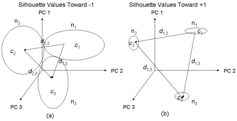
An illustration of clustering that would result in a) silhouette values tending toward −1 (poor clustering) and b) silhouette values tending toward +1 (good clustering). From Equation 8, c represents the average distance between the observation and other observations within its own cluster, and d represents the average distances between the observation and each of the other clusters. Large values for c and small values of d are required for silhouette values tending toward −1 while small values for c and large values of d are required for silhouette values tending toward +1.

ARFI and immunohistochemistry data

Two-dimensional (2D) ARFI imaging was performed using a Siemens Sonoline Antares^™ Ultrasound Scanner (Siemens Medical Solutions, Ultrasound Division, Issaquah, WA, USA) on an iliac artery of an adult FH pig in vivo. Using a VF7-3 linear array transducer, ARFI imaging was performed at a center frequency of 4.21 MHz and at a focal depth of 2.6 cm. The lateral field of view (FOV) spanned 2.1 cm by 40 ARFI impulses spaced 0.53 mm apart. The pig was sedated for imaging in agreement with the Institutional Animal Care and Use Committee (IACUC) at the University of North Carolina at Chapel Hill. A marker of the transducer location during imaging was tattooed on the animal’s skin as to spatially correlate imaging with histology. Once the ARFI data was obtained, a polynomial motion filter based on a quasi-static rigid wall model (Fung 1993) was employed to reduce displacement profile distortions from physiological motion. At each axial location of the image, the polynomial motion filter first arranges all ARFI displacement profiles in the order of acquisition through time. The resulting gross displacement profile for each depth provides an estimate of gross physiological motion of the vessel through the entirety of image acquisition. A polynomial is then fit to each axial depth gross displacement profile, and the shape of that curve is subtracted from the ARFI profiles at the same depth to remove physiologic motion. The ARFI data was further processed with a masking of displacement profiles that corresponded to blood inside the arterial lumen.

A detailed description for the immunohistochemistry staining of the FH pig iliac artery is provided in Behler et al. (2006). Briefly, the vessel is first cut longitudinally to expose the inner surface of the lumen. Sections that were in plane with the corresponding ARFI and B-mode images were stained with hematoxylin and eosin for baseline, Verhoeff van Gieson (VVG) for elastin, and Masson’s trichrome for collagen.

A region of interest was first identified for classification along the proximal wall for the in vivo FH pig iliac artery. ROBPCA followed by ROBCLUST were preformed on the data set to classify the ARFI data.

Results

Synthetic data, no outliers

Figure 5 depicts peak displacement and time to 67% recovery images for the no outlier, high noise, ST 1 synthetic tissue data set. Typical simulated displacement curves for each synthetic tissue layer are depicted in Fig. 4a. As visualized in these images, each layer (upper tissue, middle tissue, and lower tissue) is characterized by varied peak (1.3, 1.0, 0.7) and recovery rate (0.05, 0.2, 0.05) parameters.

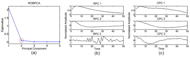
Figure 7a shows the scree plot and Fig. 7b shows the corresponding 3 most energetic robust principal components (RPC) obtained from ROBPCA as performed on the outlier void, high noise, synthetic tissue data set ST 1. The corresponding three most energetically significant classic principal components (CPC) are displayed in Fig. 7c. Note from Fig. 7a that while there are a total of 50 principal components, we elect to display only the first 5 in order to better illustrate the point of inflection from the plot. As depicted by the red circle around PC 2 in Fig. 7a, the point of inflection corresponds to PC 2, and we choose to keep the first 2 principal components. From visual analysis of the principal components in Fig. 7b, we confirm that PC 2 is an appropriate choice, as the third most energetic principal component describes variance in the noise. The first 2 most energetic principal components explain variance in the typical measured tissue response to ARFI excitation and are kept for computing robust score values and clustering.

Fig. 7.

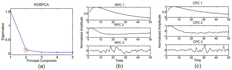
a) A robust scree plot computed from ROBPCA for the outlier void, high noise, ST 1 data set with b) the corresponding 3 most energetic robust principal components (RPC) and c) the corresponding 3 most energetic classic principal components (CPC). The red circle in 7(a) indicates the point of inflection at the second principal component.

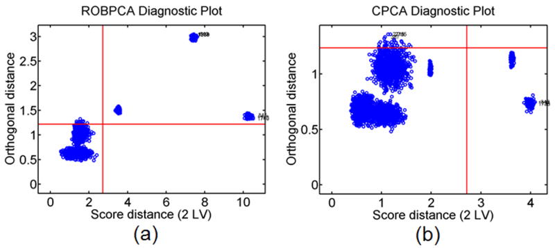
Figure 8a and 8b illustrate the method for outlier classification via diagnostic plots when both ROBPCA (Fig. 8a) and CPCA (Fig. 8b) are preformed on the no outlier, high noise, ST 1 data set. Thresholds for orthogonal and score distance values are shown as red horizontal and vertical lines. The numbers labeling selected observations indicate the synthetic displacement curves with the three largest orthogonal and score distances. Note that with no outliers in the data set, the diagnostic plots for ROBPCA and CPCA are nearly identical. One false outlier is detected (observation 2414) for both ROBPCA and CPCA methods. Fig. 8c demonstrates an example plot of silhouette values for each observation following our ROBPCA plus ROBCLUST methods, arranged in order of decreasing silhouette value per cluster.

Fig. 8.

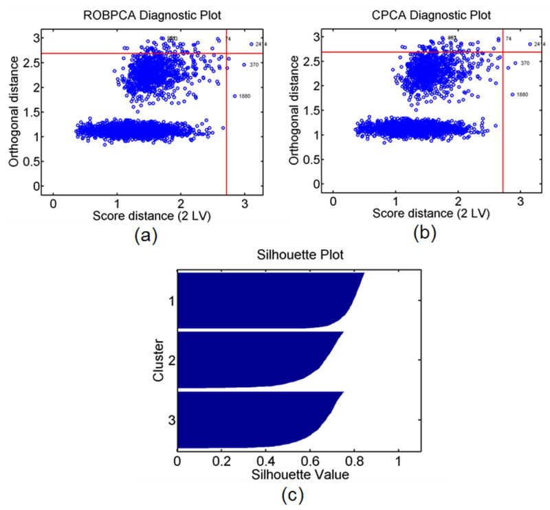
a) Diagnostic plot computed from ROBPCA and b) CPCA for the no outlier, high noise, ST 1 data set. Thresholds (red lines) are drawn for each distance such that exceeding each threshold is expected to have less than 2.5% probability. The index numbers labeling selected observations correspond to the simulated displacement curves with the 3 largest orthogonal and score distances. c) An example silhouette plot is shown for clustering with ROBCLUST.

A summary of results from each of the six classification methods operating on six unique no outlier synthetic tissue data sets is given in Table 2. Values are listed as mean percent correct or mean silhouette values ± standard deviation over 100 repetitions. Note that variance in repeated classification results were due to variations in cluster algorithm performance and occurred only in select cases utilizing PAM clustering. There are 3 instances in Table 2 where PAM clustering produces variance in classification results over 100 runs. This small amount of variance occurs in PAM clustering methods due to randomness in choosing the location of the initial cluster centroids. While we do not see variation in our K-means clustering results, clustering centroids in K-means are likewise chosen at random, which could potentially create similar variations seen from PAM clustering over a larger number of runs.

Table 2.

Classification result summary for no outlier synthetic tissue data sets

High noise, No Outliers
	ST 1		ST 2		ST 3
Method	Percent Correct	Mean Silhouette	Percent Correct	Mean Silhouette	Percent Correct	Mean Silhouette
CPCA + K-means	99.97%	0.7616	92.97%	0.4420	99.43%	0.7083
ROBPCA + K-means	99.93%	0.7603	92.90%	0.4426	99.53%	0.7087
CPCA + PAM	99.23%	0.7512	93.03%	0.4417	97.75 ± 0.55%	0.6875 ± 0.0073
ROBPCA + PAM	98.67%	0.7410	92.95 ± 0.051%	0.4422 ± 0.00015	97.78 ± 0.50%	0.6883 ± 0.0066
CPCA + ROBCLUST	99.93%	0.7579	92.97%	0.4420	99.43%	0.7084
ROBPCA + ROBCLUST	99.97%	0.7579	92.90%	0.4426	99.53%	0.7088
Moderate noise, No Outliers
	ST 1		ST 2		ST 3
Method	Percent Correct	Mean Silhouette	Percent Correct	Mean Silhouette	Percent Correct	Mean Silhouette
CPCA + K-means	100.00%	0.8668	99.87%	0.6493	100.00%	0.8323
ROBPCA + K-means	100.00%	0.8668	99.87%	0.6500	100.00%	0.8324
CPCA + PAM	100.00%	0.8668	99.87%	0.6493	99.997 ± 0.010%	0.83229 ± 0.00009
ROBPCA + PAM	100.00%	0.8668	99.86%	0.6500	99.998 ± 0.007%	0.83233 ± 0.00006
CPCA + ROBCLUST	100.00%	0.8668	99.87%	0.6493	100.00%	0.8323
ROBPCA + ROBCLUST	100.00%	0.8668	99.87%	0.6500	100.00%	0.8324

Synthetic data set, with outliers

Figure 9 displays peak displacement and time to 67% recovery images for the outlier, moderate noise, ST 1 data set. Typical displacement curves for each outlier tissue region and viscoelastic synthetic tissue layer are depicted in Fig. 4b. As shown in these images, each synthetic tissue layer (upper tissue, middle tissue, and lower tissue) contains 900 synthetic viscoelastic tissue displacement curves (described by eqns 1, 2, and 3) and 100 synthetic outlier tissue displacement curves collected from ARFI pig data.

Fig. 9.

a) Peak displacement and b) time to 67% recovery images for the outlier, moderate noise, ST 1 data set.

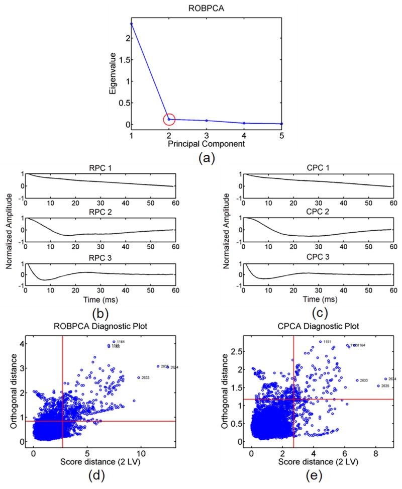
Figure 10a shows a scree plot calculated from ROBPCA while Fig. 10b displays the corresponding 3 most energetically significant robust principal components, and Fig. 10c displays the corresponding 3 most energetically significant classic principal components. Again, we choose to keep the first 2 most energetically significant robust principal components for classification as this corresponds to the inflection point from the scree plot (red circle in Fig. 10a). This is confirmed as an appropriate choice from Fig. 10b as the variance explained by the third robust principal component is purely in the noise, whereas the first 2 robust principal components explain variance in the typical measured response of viscoelastic tissue to ARFI excitation.

Fig. 10.

a) A robust scree plot computed from ROBPCA for the outlier, moderate noise, ST 1 data set with b) the corresponding 3 most energetic robust principal components (RPC) and c) the corresponding 3 most energetic classic principal components (CPC). The red circle in 10(a) indicates the point of inflection at the second principal component.

Figure 11a shows an outlier diagnostic plot when ROBPCA methods have operated on the outlier, moderate noise, ST 1 data set while Fig. 11b depicts the outlier diagnostic plot when CPCA methods are used. The orthogonal and score distance thresholds are shown as red horizontal and vertical lines. Note that the diagnostic plots for ROBPCA and CPCA become very different when the data is contaminated with outliers. The three groups of synthetic outlier tissue regions (upper outlier tissue, middle outlier tissue, and lower outlier tissue) are clearly identified only in the ROBPCA case as the three groups of observations beyond the red cutoff lines (in the upper right quadrant) in Fig. 11a.

Fig. 11.

a) Diagnostic plot computed from ROBPCA and b) CPCA for an outlier containing, moderate noise, ST 1 data set. Thresholds (red lines) are drawn for each distance such that exceeding each threshold is expected to have less than 2.5% probability.

A summary of the classification performance for each of the six methods operating on six unique outlier data sets are given in Table 3. Values are listed as mean percent correct or mean silhouette values ± standard deviation over 100 repetitions.

Table 3.

Classification result summary for outlier tissue containing synthetic data sets

High noise, Outliers
	ST 1		ST 2		ST 3
Method	Percent Correct	Mean Silhouette	Percent Correct	Mean Silhouette	Percent Correct	Mean Silhouette
CPCA + K-means	63.33%	0.8041	33.33%	0.8705	66.67%	0.7980
ROBPCA + K-means	63.33%	0.8034	63.20%	0.5233	66.67%	0.7954
CPCA + PAM	92.23%	0.6248	33.33%	0.8705	89.84 ± 0.93%	0.4860 ± 0.0272
ROBPCA + PAM	92.77%	0.6320	86.33%	0.3568	90.52 ± 0.08%	0.5191 ± 0.0187
CPCA + ROBCLUST	63.33%	0.7799	36.67%	0.8511	66.67%	0.7444
ROBPCA + ROBCLUST	63.20%	0.7799	89.27%	0.4350	66.67%	0.7436
Moderate noise, Outliers
	ST 1		ST 2		ST 3
Method	Percent Correct	Mean Silhouette	Percent Correct	Mean Silhouette	Percent Correct	Mean Silhouette
CPCA + K-means	66.67%	0.8335	33.33%	0.8841	66.67%	0.8233
ROBPCA + K-means	62.23%	0.8164	63.33%	0.6070	66.67%	0.8264
CPCA + PAM	90.00%	0.7052	33.33%	0.8855	89.87%	0.6192
ROBPCA + PAM	90.00%	0.7182	89.87%	0.4734	90.00%	0.6416
CPCA + ROBCLUST	66.67%	0.7979	36.67%	0.8653	66.67%	0.7582
ROBPCA + ROBCLUST	100.00%	0.8669	99.87%	0.6524	100.00%	0.8290

The computational time for each of the six methods operating on the outlier, moderate noise, ST 1 data set over 100 runs was measured on a 1.5-GHz Pentium M processor. The computational time results are summarized in Table 4 along with the ratios of percent correct values from Table 3 to computational time for each technique.

Table 4.

Average computation times for classification methods. Ratio of percent correct results from Table 3 for the ST 1, outlier, moderate noise data sets to computational time.

Method	Mean CPU Time (s) ± Standard Deviation	(Moderate Noise Percent Correct/Mean CPU Time) ± Standard Deviation
CPCA + K-means	0.9525 ± 0.0710	69.8787 ± 7.3274
ROBPCA + K-means	6.4509 ± 0.2428	9.6029 ± 0.6619
CPCA + PAM	16.3766 ± 0.1755	5.4917 ± 0.0730
ROBPCA + PAM	26.2128 ± 0.4710	3.4338 ± 0.0587
CPCA + ROBCLUST	11.6593 ± 0.6770	5.7278 ± 0.3432
ROBPCA + ROBCLUST	12.5812 ± 0.4708	7.9520 ± 0.3024

In vivo FH pig iliac artery

Figure 12a illustrates a scree plot calculated from ROBPCA for ARFI data from an in vivo FH pig iliac artery within the ROI. The corresponding 3 most energetically significant robust principal components are displayed in Fig. 12b while the corresponding 3 most energetically significant classic principal components are displayed in Fig. 12c. The number of robust principal components to retain was again determined by the inflection point of the scree plot (red circle in Fig. 12a). The corresponding outlier diagnostic plots calculated from ROBPCA and CPCA approaches are displayed in Fig. 12d and Fig. 12e, respectively. Threshold lines are marked in red so that the probability of exceeding each distance is expected to be less than 2.5%.

Fig. 12.

a) A robust scree plot computed from ROBPCA for the in vivo FH pig iliac artery data set with b) the corresponding 3 most energetic robust principal components (RPC) and c) the corresponding 3 most energetic classic principal components (CPC). The red circle in 12(a) indicates the point of inflection at the second principal component. Outlier diagnostic plots from ROBPCA and CPCA are shown in 12(d) and (e) respectively. Thresholds (red lines) are drawn for each distance such that exceeding each threshold is expected to have less than 2.5% probability.

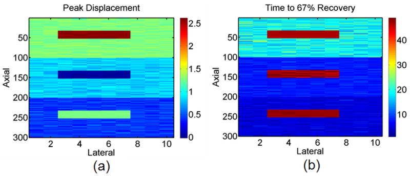
Table 5 summarizes the mean silhouette values produced from each of the six classification methods as preformed on the in vivo FH pig iliac data within the ROI. In Figure 13 B-mode, ARFI peak displacement, and ARFI time to 67% recovery images are displayed for an in vivo FH pig iliac artery. The ROI for classification is illustrated in Fig. 13a as a red box around the proximal wall. The classification results from our ROBPCA plus ROBCLUST algorithm are viewed in Figure 13d and 13e. The number of clusters was chosen for classification by visual analysis between classification, immunohistochemistry results, and parametric ARFI images, and the robust scores were clustered into 6 segments. In Fig. 13d the cluster groups are colored by average peak displacement while in Fig. 13e the cluster groups are colored by average time to 67% recovery. Note that this coloring in no way effected classification and only served to highlight key ARFI parameters of interest. Fig. 13f displays the average displacement profile for each of the six cluster segments where the color of each profile is matched to the classification by time to 67% recovery image in Fig. 13e. Fig. 13g displays the clustered robust score values for robust principal components 1 and 2 where color is again matched to the image in Fig. 13e. Boxes 1, 2, and 3 are labeled across ARFI images in Fig. 13b and 13c to spatially match those shown for the histological sections in Fig. 14 and classification images in Fig. 13d and 13e.

Table 5.

Average silhouette values for in vivo FH pig iliac artery data

Method	Mean Silhouette Value
CPCA + K-means	0.3790
ROBPCA + K-means	0.3825
CPCA + PAM	0.3691
ROBPCA + PAM	0.3715
CPCA + ROBCLUST	0.3881
ROBPCA + ROBCLUST	0.4087

Fig. 13.

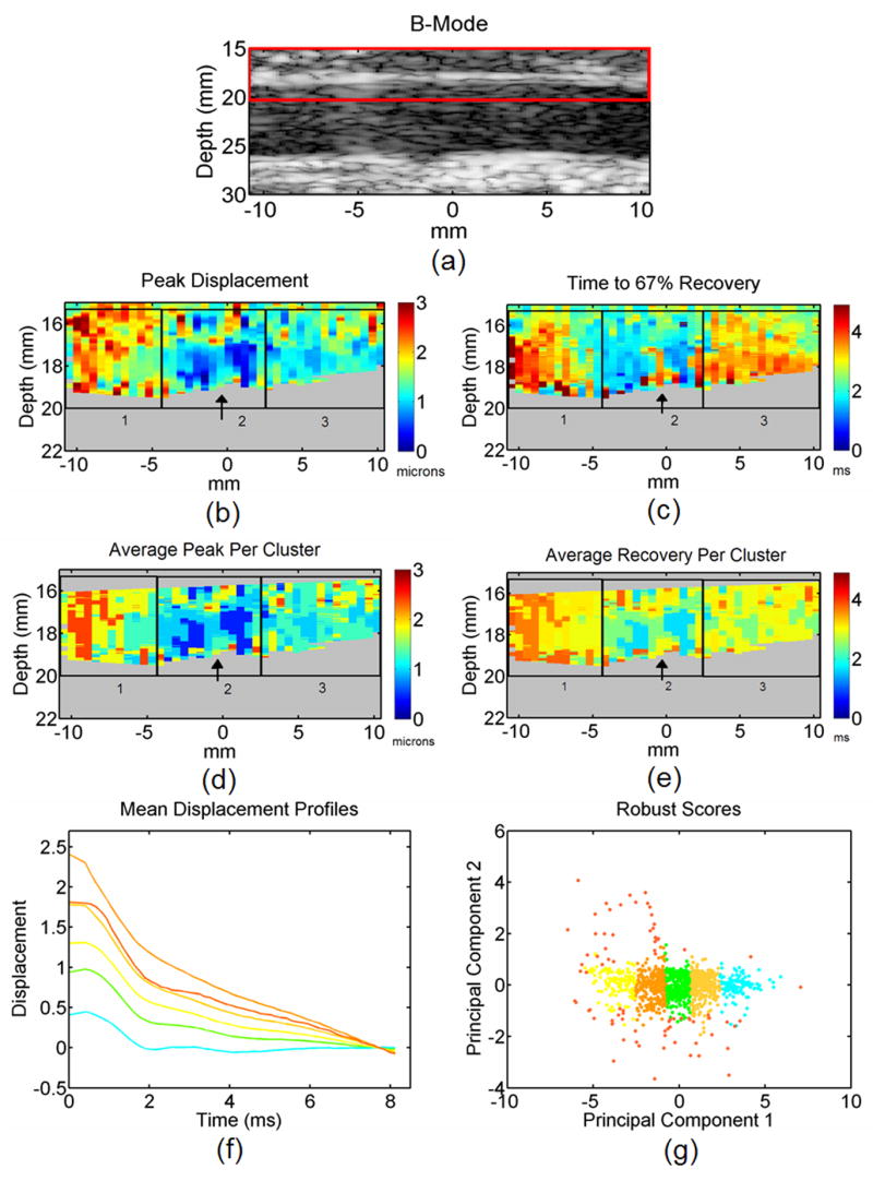
a) A B-mode, b) ARFI peak displacement, and c) ARFI time to recovery image for an in vivo FH pig iliac artery. The red box in 13(a) depicts the ROI for classification. Color indicates peak displacement in microns for 13(b) and time to 67% recovery in milliseconds for 13(c). ARFI data classified by ROBPCA and ROBCLUST for 6 clusters are indexed by d) average peak displacement and e) average time to 67% recovery. Boxes 1, 2, and 3 in 13(d) and (e) are spatially matched to histology in Fig. 14 and parametric ARFI images in 13(b) and (c). The black arrow in box 2 indicates the location of suspected elastin dropout from histological inspection in Fig. 14. Mean displacement profiles for each of the 6 cluster groups are displayed in 13(f) while clustered robust score values are depicted in 13(g). Both 13(f) and 13(g) are colored to match cluster groups for the average time to 67% recovery image in 13(e). ARFI imaging was performed at a focal depth of 2.6 cm.

Fig. 14.

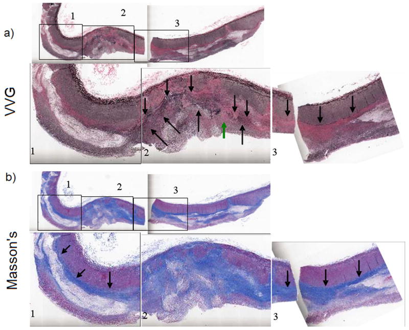
An in vivo FH pig iliac artery sectioned and stained with a) Verhoeff von Gieson (VVG) for elastin and b) Masson’s Trichrome for collagen. Boxes 1, 2, and 3, are shown at higher magnification for a more detailed view of the histology. The boxes are spatially consistent with the labeled boxes in parametric ARFI (Fig. 13(b) and 13(c)) and classification images (Fig. 13(d) and 13(e)). The green arrow in 14(a) indicates the location of suspected elastin dropout.

Verhoeff von Gieson (VVG) staining for elastin is displayed in Fig. 14a, and Masson’s trichrome staining for collagen is viewed in Fig. 14b. A spatial correlation between ARFI results and immunohistochemistry has already been reported in Behler et al. (2006).

Discussion

We have examined 6 different classification methods combining classical PCA or robust PCA data decompositions with K-means, PAM, or ROBCLUST clustering methods. These methods operated on synthetic tissue data sets that varied in terms of additive noise and outlier tissue content as well as in terms of simulated displacement curve peak displacement and recovery time parameters. Synthetic tissue data set 1 (ST 1) included tissue layers with distinct peak displacement and recovery rate parameters, ST 2 consisted of tissue layers that exhibited variation only in terms of peak displacement parameters, and ST 3 included tissue layers that exhibited variation only in terms of recovery rates.

Consider the case of synthetic tissue that contains no outliers (Fig. 5). We observe two predominant trends. First, CPCA and ROBPCA approaches to data decomposition perform equally well, in general, as indicated by diagnostic plots generated in the case of both high and moderate noise levels, as well as in the case of ST 1, ST 2, and ST 3. For example, the diagnostic plots depicted in Fig. 8a and 8b for ROBPCA and CPCA, respectively, in the case of high noise and ST 1 are nearly identical, with both detecting the same false positive (displacement curve indexed 2414) in the upper right quadrant. Moreover, silhouette and percent correct values, reported in Table 2, indicate nearly equivalent performance of ROBCLUST classification independent of CPCA or ROBPCA decomposition method. This result meets our expectation that when no outliers are present in the data set, ROBPCA produces basis functions that are highly similar to the basis functions produced by CPCA. A second notable trend is that K-Means, PAM, and ROBCLUST methods for displacement curve classification yield similar performances in terms of percent correct and silhouette values, as reported in Table 2. For all three methods, classification performance increases, i.e. percent correct and silhouette values increase, as noise level decreases. In addition, classification performance is best when both peak displacement and recovery time parameters vary between tissue layers (ST 1) and worst when only peak displacement differs between layers (ST 3).

Now consider the case of synthetic tissue data with outlier tissue regions (Fig. 9). Again we observe two predominate trends. First, CPCA and ROBPCA approaches perform differently when the data contains 10% outliers. This is observed by visual inspection of the basis functions in Fig. 10 and is further reflected by differences in diagnostic plots generated in the case of both high and moderate noise levels, as well as in the case of ST 1, ST 2, and ST 3. For example, the moderate noise, ST 1 diagnostic plots in Fig. 11a and Fig. 11b produced by ROBPCA and CPCA, respectively, are noticeably different. Whereas ROBPCA basis functions identify the three regions of synthetic outlier tissue beyond the distance thresholds (Fig. 11a), CPCA basis functions do not identify any outliers in the data. Furthermore, percent correct and silhouette values, reported in Table 3, generally indicate superior performance of ROBCLUST when operating on ROBPCA-derived score values as opposed to CPCA-derived score values. This result meets our expectations that when outliers are present in the data, ROBPCA produces robust basis functions, which identify outliers that cannot be detected when the data is decomposed via CPCA.

Second, we observe the trend that ROBCLUST generally yields superior performance than PAM, which generally yields superior performance than K-Means in terms of percent correct and silhouette values, as reported in Table 3. The exceptions to this trend occur in both high noise, ST 1 and high noise, ST 3 data sets where PAM clustering yields superior results to both K-Means and ROBCLUST. In these instances (high noise, ST 1 and ST 3), a large amount of noise is added to a data sets already containing 10% outlier tissue. The resulting basis functions describe much less variance in the typical measured response to ARFI excitation and much more variance in random additive noise. Therefore, ROBPCA becomes unable to correctly identify outlier tissue regions in the data set, and ROBCLUST is likewise unable to separate outlier score values from normal observation score values. For all three methods, performance generally increases, i.e. percent correct and silhouette values generally increase, as noise level decreases. Unlike the results reported for the outlier void data set in Table 2, there is no clear trend for performance between the high noise and ST 1, ST 2, and ST 3 data sets reported in Table 3.

Our synthetic data results support that robust PCA and clustering methods perform better than classical PCA, conventional K-Means, and PAM methods in the case of data inclusive of outliers and moderate noise. To compare the performance of these methods in an in vivo imaging environment, we are limited to analysis of diagnostic plots and silhouette values, as measurement of percent correct is not possible in the absence of a true gold standard.

First, observe the basis functions produced from the in vivo FH pig iliac artery data for ROBPCA and CPCA methods in Fig. 12b and Fig. 12c, respectively. By careful visual inspection it is observable that ROBPCA and CPCA basis functions are slightly dissimilar in general shape. This dissimilarity is further reflected by visual analysis of the ROBPCA and CPCA diagnostic plots in Fig. 12d and Fig. 12e, respectively. From inspection of these diagnostic plots, it is clear that data decomposition by ROBPCA labels many more outlier displacement profiles beyond the threshold distance values than data decomposition by CPCA.

Now observe the mean silhouette values reported in Table 5 from classification results via our six distinct methods. Recall that a silhouette value is a metric that reflects dissimilarity of ARFI displacement profiles between assigned clusters versus similarity of ARFI profiles within clusters. A higher silhouette value suggests greater profile similarity within versus between clusters. Two main trends are observed from the mean silhouette value data reported in Table 5. First, classification via ROBPCA yields larger silhouette values than classification achieved by CPCA, and second, classification results are best with ROBCLUST clustering methods and worst with PAM clustering methods. Overall, we observe that the combination of ROBCPA and ROBCLUST methods outperforms the alternative methods in terms of mean silhouette values reported in Table 5.

We can further assess the performance of our combined ROBPCA and ROBCLUST classification methods by comparing the resulting classification images to parametric ARFI images and histology. The reader is referred to Behler et al. (2006) for a more detailed description of the ARFI images and their correlation to the spatially matched immunohistochemistry. It is visually discernable that our classification results (Fig. 13d and 13e) are comparable to the parametric ARFI images depicting peak induced displacement and time to recovery from peak induced displacement in Fig. 13b and 13c, respectively. In both parametric ARFI and classification ARFI images, the tissue region in box 1 generally exhibits relatively large peak displacement and slow recovery, while that in box 2 shows relatively small peak displacement and fast recovery.

More specifically, from our classification results in Fig. 13d and 13e, we see a decrease in average time to 67% recovery (orange to yellow, ~3.5 to 3 ms) and average peak displacement (red to light green, ~2.4 to 1.3 μm) from left to right across box 1. This is spatially consistent with immunohistochemistry from Fig. 14 which shows an increase in elastin and collagen composition across the same region. Box 2 is dominated primarily by the light blue and light green classifications in Fig. 13e, which exhibit short recovery times (light blue and green, ~2 and 2.5 ms). This is spatially consistent with the pronounced deposition of elastin in this tissue region. There is also a small region in the middle of box 2 along the vessel wall that consists of slower average recovery rates (yellow and orange, arrow, ~ 3 and 3.5 ms), which would agree with the elastin drop-out described from Fig. 14a (green arrow). Similarly, box 2 shows relatively smaller average peak displacement in Fig. 13d (blue and light blue, ~0.5 and 1.0 μm), consistent with the general collagen deposition depicted in this region in Fig. 14b. In agreement with a more homogenous internal elastic lamina seen in Fig. 14a, there is a largely uniform recovery rate in box 3 which is dominated by the yellow and light green classifications (~3 and 2 ms) in Fig. 13e. Likewise, box 3 is dominated by the light green and light blue regions (~1.3 and 1.0 μm) for the classification by average peak displacement image in Fig. 13d. These classifications show less peak displacement than the red and yellow (~2.4 and 1.8 μm) regions that dominate box 1 but show more peak displacement than the blue region seen in box 2 (~0.5 μm). Once more, this result correlates with the relative amount of collagen content seen in box 3 from Masson’s staining in Fig. 14b.

Note that while statistically based approaches, such as principal component analysis, are often taken in signal and image processing, they are susceptible to unintended signal distortions. We point out, however, that though a highest-energy subset of principal components are selected to govern profile classification, the profiles themselves are not in any way altered by our analysis. Unintended image distortions are therefore limited to improper classifications of tissue regions exhibiting similar response to ARFI excitation. The tissue response itself remains unchanged. While statistical relationships based on physical relationships are most favorable, carefully monitored statistical constraints are appropriate until the physics of the measurements are better understood.

Conclusions

We have demonstrated an automated, robust classification algorithm for in vivo vascular ARFI data classification utilizing a robust principal component (ROBPCA) algorithm and a modified robust K-means (ROBCLUST) clustering technique. Our synthetic tissue experiments have shown that these robust techniques yielded improved classification outcomes in comparison to alternative PCA plus clustering methods in the presence of moderate to high noise content (10dB to 5dB average SNR to amplitude), excluding synthetic outlier tissue. In addition in the context of 10% synthetic outlier tissue, our techniques outperformed other classification methods in the case of moderate noise levels. However, robust PCA and cluster performance was degraded in the case of outliers and high noise levels (5dB average SNR to amplitude). When applied to an in vivo ARFI data set acquired in an FH pig iliac artery, ROBPCA identified more outlier profiles than CPCA, and the combined ROBPCA and ROBCLUST approach yielded higher mean silhouette values than the other examined methods. Our resulting classification images from the combined ROBPCA and ROBCLUST methods were visually comparable to parametric ARFI images and were consistent with matched immunohistochemistry. Notably, these robust methods provided more information than traditional ARFI data analysis via automatic identification of outlier displacement profiles in the data set and automatic grouping of displacement profiles with similar profile shapes. Note that we have presented techniques that do not impose spatial smoothness constraints on the clustering algorithm solutions. In future work, we plan to incorporate spatial information into clustering methods, implement our algorithm in other clinical environments, automate cluster number selection, and examine alternatives to robust PCA for ARFI displacement profile dimensionality reduction. Beyond demonstration of ARFI data classification, these studies provide an important step toward statistically relating ARFI results to immunohistochemical data. Future work will also focus on developing these methods to correlate ARFI data to histology.

References

- Alizad A, Fatemi M, Wold LE, Greenlead JF. Performance of vibroacoustography in detecting microcalcifications in excised human breast tissue: A study of 74 tissue samples. IEEE Trans Med Imaging. 2004;23(3):307–312. doi: 10.1109/TMI.2004.824241. [DOI] [PubMed] [Google Scholar]
- Baldeswing RA, Mastik F, Schaar JA, Serruys PW, van der Steen AFW. Young’s modulus reconstruction of vulnerable atherosclerotic plaque components using deformable curves. Ultrasound Med Biol. 2006;32(2):201–210. doi: 10.1016/j.ultrasmedbio.2005.11.016. [DOI] [PubMed] [Google Scholar]
- Behler RH, Nichols TC, Merricks EP, Dumont DM, Gallippi CM. ARFI characterization of atherosclerosis. IEEE Ultrasonics Symposium. 2006:722–727. [Google Scholar]
- Bercoff J, Pernot M, Tanter M, Fink M. Monitoring thermally-induced lesions with supersonic shear imaging. Ultrason Imaging. 2004;26(2):71–84. doi: 10.1177/016173460402600201. [DOI] [PubMed] [Google Scholar]
- Brusseau E, de Korte CL, Mastik F, Schaar J, van der Steen AFW. Fully automatic luminal contour segmentation in intracoronary ultrasound imaging. IEEE Trans Med Imaging. 2004;23(5):554–566. doi: 10.1109/tmi.2004.825602. [DOI] [PubMed] [Google Scholar]
- Dahl JJ, Dumont DM, Miller EM, Allen JD, Trahey GE. Characterization of in vivo atherosclerotic plaques in the carotid artery with acoustic radiation force impulse imaging. IEEE Ultrasonics Symposium. 2006:706–709. [Google Scholar]
- Dumont DM, Behler RH, Nichols TC, Merricks EP, Gallippi CM. ARFI imaging for noninvasive material characterization of atherosclerosis. Ultrasound Med Biol. 2006;32(11):1703–1711. doi: 10.1016/j.ultrasmedbio.2006.07.014. [DOI] [PubMed] [Google Scholar]
- Fahey BJ, Nightingale KR, Stutz DL, Trahey GE. Acoustic radiation force impulse imaging of thermally- and chemically-induced lesions in soft tissues: Preliminary ex vivo results. Ultrasound Med Biol. 2004;30(3):321–328. doi: 10.1016/j.ultrasmedbio.2003.11.012. [DOI] [PubMed] [Google Scholar]
- Fahey BJ, Nightingale KR, McAleavey SA, Palmeri ML, Wolf PD, Trahey GE. Acoustic radiation force impulse imaging of myocardial radiofrequency ablation: Initial in vivo results. IEEE Trans Ultrason Ferroelectr Freq Control. 2005;52(4):631–641. doi: 10.1109/tuffc.2005.1428046. [DOI] [PubMed] [Google Scholar]
- Fahey BJ, Nightingale KR, Nelson RC, Palmeri ML, Trahey GE. Acoustic radiation force impulse imaging of the abdomen: Demonstration of feasibility and utility. Ultrasound Med Biol. 2005;31(9):1185–1198. doi: 10.1016/j.ultrasmedbio.2005.05.004. [DOI] [PubMed] [Google Scholar]
- Fukunaga K. Introduction to statistical pattern recognition. 2. Elsevier; 1990. [Google Scholar]
- Fung YC. Biomechanics: mechanical properties of living tissues. Springer; 1993. [Google Scholar]
- Gallippi CM, Trahey GE. Adaptive clutter filtering via blind source separation for two-dimensional ultrasonic blood velocity measurement. Ultrason Imaging. 2002;24(4):193–214. doi: 10.1177/016173460202400401. [DOI] [PubMed] [Google Scholar]
- Gallippi CM, Nightingale KR, Trahey GE. BSS-based filtering of physiological and arfi-induced tissue and blood motion. Ultrasound Med Biol. 2003;29(11):1583–1592. doi: 10.1016/j.ultrasmedbio.2003.07.002. [DOI] [PubMed] [Google Scholar]
- Gallippi CM, Trahey GE. Complex blind source separation for acoustic radiation force impulse imaging in the peripheral vasculature, in vivo. IEEE Ultrasonics Symposium. 2004:596–601. [Google Scholar]
- Hubert M, Rousseeuw PJ, Brandon KV. ROBPCA: a new approach to robust principal component analysis. Technometrics. 2005;47(1):64–79. [Google Scholar]
- Kaufman L, Rousseeuw PJ. Finding groups in data: an introduction to cluster analysis. Wiley-Interscience; 1990. [Google Scholar]
- Levy JH, Behler R, Haider MA, Marron JS, Gallippi CM. Discrimination of Kelvin materials via ARFI response. 9th MICCAI Conference Proceedings; Copenhagen Denmark. 2006. in press. [Google Scholar]
- Mauldin FW, Levy JH, Behler RH, Nichols J, Marron S, Gallippi CM. Blind source separation and k-means clustering for vascular ARFI image segmentation, in vivo and ex vivo. IEEE Ultrasonics Symposium. 2006:1666–1671. [Google Scholar]
- Maurice RL, Daronat M, Ohayon J, Stoyanova E, Foster FS, Cloutier G. Non-invasive high-frequency vascular ultrasound elastography. Phys Med Biol. 2005;50:1511–1628. doi: 10.1088/0031-9155/50/7/020. [DOI] [PubMed] [Google Scholar]
- McKay CR, Shavelle DM. Intravascular ultrasound in the coronary arteries. Semin Vasc Surg. 2006;19(3):132–138. doi: 10.1053/j.semvascsurg.2006.06.007. [DOI] [PubMed] [Google Scholar]
- Mozes G, Kinnick RR, Gloviczki P, Bruhnke RE, Carmo M, Hoskin TL, Bennet KE, Greenleaf JF. Noninvasive measurement of aortic aneurysm sac tension with vibrometry. J Vasc Surg. 2005;42(5):963–971. doi: 10.1016/j.jvs.2005.07.012. [DOI] [PubMed] [Google Scholar]
- Nightingale KR, Soo MS, Nightingale R, Trahey GE. Acoustic radiation force impulse imaging: in vivo demonstration of clinical feasibility. Ultrasound Med Biol. 2002;28(2):227–235. doi: 10.1016/s0301-5629(01)00499-9. [DOI] [PubMed] [Google Scholar]
- O’Rourke J, Toussaint GT. Handbook of discrete and computational geometry. 2. Chapman & Hall/CRC; 2004. [Google Scholar]
- Palmeri ML, Frinkley KD, Zhai L, Gottfried M, Bentley RC, Ludwig K, Nightingale KR. Acoustic radiation force impulse (ARFI) imaging of the gastrointestinal tract. Ultrason Imaging. 2005;27(2):75–88. doi: 10.1177/016173460502700202. [DOI] [PubMed] [Google Scholar]
- Soo MS, Ghate SV, Baker JA, Rosen EL, Walsh R, Warwick BN, Ramachandran AR, Nightingale KR. Streaming detection for evaluation of indeterminate sonographic breast masses: A pilot study. Am J Roentgenol. 2006;186(5):1335–1341. doi: 10.2214/AJR.05.0005. [DOI] [PubMed] [Google Scholar]
- Trahey GE, Palmeri ML, Bentley RC, Nightingale KR. Acoustic radiation force impulse imaging of the mechanical properties of arteries: In vivo and ex vivo results. Ultrasound Med Biol. 2004;30(9):1163–1171. doi: 10.1016/j.ultrasmedbio.2004.07.022. [DOI] [PubMed] [Google Scholar]
- Tuczu EM, Schoenhagen P. Atherosclerosis imaging: Intravascular ultrasound. Drugs. 2004;64 (Suppl 2):1–7. doi: 10.2165/00003495-200464002-00002. [DOI] [PubMed] [Google Scholar]
- Verboven S, Hubert M. LIBRA: a Matlab library for robust analysis. Chemometrics and intelligent laboratory systems. 2005;75:127–135. [Google Scholar]
- Viola F, Kramer MD, Lawrence MB, Oberhauser JP, Walker WF. Sonorheometry: A noncontact method for the dynamic assessment of thrombosis. Ann Biomed Eng. 2004;32(5):696–705. doi: 10.1023/b:abme.0000030235.72255.df. [DOI] [PubMed] [Google Scholar]
- Zhang XM, Greenleaf JF. Noninvasive generation and measurement of propagating waves in arterial walls. J Acoust Soc Am. 2006;119(2):1238–1243. doi: 10.1121/1.2159294. [DOI] [PubMed] [Google Scholar]