Order patterns recurrence plots in the analysis of ERP data

Abstract

Recurrence quantification analysis (RQA) is an established tool for data analysis in various behavioural sciences. In this article we present a refined notion of RQA based on order patterns. The use of order patterns is commonplace in time series analysis. Exploiting this concept in combination with recurrence plots (RP) and their quantification (RQA) allows for advances in contemporary EEG research, specifically in the analysis of event related potentials (ERP), as the method is known to be robust against non-stationary data. The use of order patterns recurrence plots (OPRPs) on EEG data recorded during a language processing experiment exemplifies the potentials of the method. We could show that the application of RQA to ERP data allows for a considerable reduction of the number of trials required in ERP research while still maintaining statistical validity.

Introduction

Electroencephalograms (EEG) provide a non-invasive tool to measure small-scale changes in the brains electric field via electrodes placed on the scalp. The main advantage of this method is its high temporal resolution, which allows studying changes in the brain’s electric field over time. The source of this measurable voltage change is the activation of a vast number of neurons in the cortex. Neurons are known to be nonlinear devices, since a certain threshold has to be crossed for the neuron to fire (Kandel et al. 1995). Certain patterns of this change are known to correlate with higher cognitive tasks such as language processing. These typical patterns are called event-related potentials (ERP) and can provide valuable insights into information processing in the brain (Donchin et al. 1978).

EEG data, though of high relevance in cognitive research, poses a number of technical problems as it is very noisy and shows strong non-stationarities. Since the amplitude of the ERP component is very small, compared to the background noise, a common approach is the use of Grand Averages, i.e. a large number of measurements is averaged in order to improve the signal-to-noise ratio (SNR). While this procedure in general highlights the component of interest, it may not be an appropriate means of analysis, because the latency of the component of interest, especially those related to higher cognitive processes such as language, may vary in time (Kutas and van Petten 1994). Further, ERPs are defined in relation to a baseline. The baseline is taken to be a period of inactivity and is most commonly calculated from the prestimulus interval.

However, it has been argued convincingly, that these preprocessing techniques are based on assumptions which are not necessarily met when dealing with real-life EEG data (cf. beim Graben et al. 2000; and references therein). Therefore an important challenge is to develop data analysis techniques that require only a few measurements, instead of large preprocessed ensembles.

To analyse EEG data with respect to its source of origin, a highly complex nonlinear system—the brain—a number of methods have been proposed amongst them symbolic dynamics (beim Graben et al. 2004), phase synchronisation analysis (Allefeld and Kurths 2004) and recurrence quantification analysis (RQA) (Marwan and Meinke 2004).

In this article we present an alternative version of RQA based on order patterns (OP) and apply it to EEG data obtained in a repetition of the meanwhile classical works of Kutas and Hillyard (1980). Order patterns are used to reencode the original EEG data as a series of symbols of which then a recurrence plot (RP) is computed. (OP)RPs capture information about the time dependent behaviour of the underlying dynamical system which can be extracted in well-defined measures of complexity. We will show that RQA based on order patterns is a promising means of analysis, because of its robustness against non-stationarities in the analysed data.

Data analysis based on recurrence plots

Recurrence is a fundamental property of complex dynamical systems. Every such system will, after a sufficiently long time, return to an arbitrarily small neighbourhood of a previous state (Poincaré 1890).

Recurrence plots

The method of RPs was introduced to visualise this time dependent behaviour of a dynamical system which can be pictured as a trajectory (i = 1, ..., N, t = i Δt, where Δt is the sampling rate) in the d-dimensional phase space (Eckmann et al. 1987). The main step of this visualisation is the calculation of an N × N-matrix

1

where ɛ is a cut-off distance and a norm (e.g. Euclidean or maximum norm). The main parameter is the cut-off distance ɛ which defines a box or sphere centred at If falls within this vicinity, the state will be close to and is considered to be a recurrence of the state (R_i,j = 1). The binary values in R_i,j can be visualised by a matrix plot with the colours black (1) and white (0).

Often there are only one-dimensional time series available. The phase space vectors x_i for a one-dimensional time series u_i can be reconstructed using the Taken’s time delay method with embedding dimension d and delay τ (Takens 1981), where the dimension d can be estimated by using methods based on false nearest neighbours (Kennel et al. 1992).

An RP exhibits characteristic large-scale and small-scale patterns which are caused by typical dynamical behaviour (Eckmann et al. 1987; Marwan et al. 2007), e.g. diagonals (similar local evolution of different parts of the trajectory) or horizontal and vertical black lines (state does not change for some time). Depending on the nature of the underlying system typical patterns can be observed (Fig. 1).

Fig. 1.

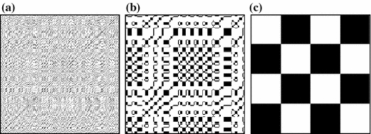
Sample OPRPs of different kinds of dynamical systems. (a) noise, (b) a chaotic system (the Lorenz attractor with ρ = 28, β = 8/3, σ = 10) and (c) a periodic signal (sine wave). The embedding parameters were m = 3, τ = 3 (a, c) and m = 3, τ = 15 (b)

The information contained in an RP can be quantified by measures of complexity based on the recurrence point density, diagonal and vertical structures in the RP (Marwan et al. 2007). The recurrence rate RR denotes the recurrence point density. Measures based on diagonal structures are the determinism DET (ratio of recurrence points forming diagonal structures to all recurrence points), the maximal length of diagonal structures L_max, their averaged length L and ENTR (the Shannon entropy of the frequency distribution of the length of the diagonal lines). Complexity measures based on vertical lines are the laminarity LAM (ratio of recurrence points forming vertical structures to all recurrence points), the maximal length of a vertical line V_max and its average TT, the so-called Trapping Time.

These measures can be computed from the whole RP or in moving windows (i.e. sub-RPs) moved along the main diagonal of the RP. The latter allows studying changes of these measures in time, which can reveal transitions in the system.

It has been shown that the RQA measures based on diagonal lines can detect transitions between chaos and order (Trulla et al. 1996), while measures based on vertical lines additionally indicate chaos-chaos transitions (Marwan et al. 2002).

Despite the valuable knowledge about dynamical systems the RQA can provide, the above introduced measures (among others) can also be used for purely diagnostical purposes. In the present article we will exploit this descriptive power of the method to discriminate different experimental conditions of a language processing experiment (cf. Table 1).

Table 1.

Sample sentences used in the experiment described

	Condition	Example
A	Control	Der Priester wurde gerufen.
		The priest was called.
B	Semantic mismatch	Der Priester wurde gepflanzt.
		The priest was planted.

Sentences like the one in B are known to elicit a negative going waveform in the EEG relative to a control sentence like A (Kutas and Hillyard 1980)

Order patterns recurrence plots

In Eq. (1) recurrence is defined by spatial closeness between points of phase space trajectories (or embedded time series u_i). Now we neglect the spatial distance in phase space and define a recurrence by using the local order structure of a trajectory. Given a one-dimensional time series, we start to compare d = 2 time instances and define the order patterns π as

2

with the scaling parameter τ. This parameter ensures that the points considered in forming the order pattern π do not show trivial dependencies. Next, for d = 3 there are six different order patterns in the triple (u_i, u_i+τ, u_{i+2 τ}) possible (Fig. 2). In general the d components in can form d! different patterns. Tied ranks (u_i =  u_i+τ) are assumed to be rare and we neglect them. From these order patterns we form a new symbolic time series π_i and define the order patterns recurrence plot (OPRP) as (Groth 2005)

3

Fig. 2.

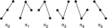
Order patterns for dimension d = 3 (tied ranks u_i =  u_i+τ are assumed to be rare)

Analogue to regular RPs from an OPRP the above introduced measures of complexity can be calculated and subjected to further statistical analysis. The main advantage of the symbolic representation is the well-expressed robustness against non-stationarity. The order patterns are invariant with respect to an arbitrary, increasing transformation of the amplitude. Furthermore a robust complexity measure based on this symbolic dynamics, the permutation entropy, was proposed (Bandt and Pompe 2002) and successfully applied to epileptic seizure detection (Cao et al. 2004).

To illustrate the invariance against such an arbitrary, increasing transformation of the amplitude we computed the RP and the OPRP for a timeseries with 150 time points derived from the logistics map (x_(n+1) = ax_n(1−x_n)). We varied the control parameter a in such a way that for the first and the last 50 time points the signal is periodic (a = 3.4), while the intermediate signal represents chaos (a = 3.89). In both the regular and the order patterns RP the transition from period to chaos can be observed clearly (Fig. 3a, b). In the next step added uniformly distributed noise (interval 0–0.4) to the signal and again computed the RP and the OPRP. While the OPRP (Fig. 3c) is virtually identical with the one observed before, the regular RP turns white (Fig. 3d) and does not detect the periodic behaviour nor the transition from period to chaos. Note that from the underlying signal we can hardly infer any information at all since the noise strongly distorts the signal. Secondly, the given signal is rather short (150 timepoints) which is problematic for other means of analysis.

Fig. 3.

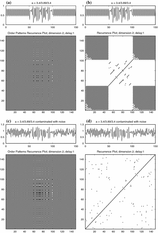
(OP)RPs for the logistics map with varying control parameters. Given an uncorrupted signal, regular and order patterns RPs detect the transition from periodic to chaotic behaviour. When the signal is contaminated with noise only the OPRP can still detect this transition. A regular RP does not detect any periodic behaviour in the signal

Materials and methods

The data used in this article has previously been examined and was kindly provided by Allefeld et al. (2005). The experimental setup was first introduced by Kutas and Hillyard (1980) and is known to elicit an N400, a negative going waveform in the EEG peaking at about 400 ms after presentation of the verb relative to the control condition. The N400 is generally associated with the process of semantic integration (Friederici 2002).

Subjects

Sixteen subjects (8 female) participated in a language processing study. All were right-handed, monolingual native speakers of German aged 20–27. To underline the capabilities of the method we focussed on one randomly selected subject. We opted for this procedure since the general assumption underlying ERP research is that the brains response to a given stimuli is observable in every (healthy) brain. Second, the present article is to be seen as a proof of concept, rather than an ERP study, which is why we consciously focussed on the methodological part our work. Nonetheless, we were able to verify the results illustrated here at other electrodes sites and with other subjects. A more detailed analysis will be presented in a forthcoming article.

Procedure

The stimulus material was presented in a word-by-word fashion on a 17” computer screen. The language material consisted of 52 pairs of sentences. From the correct German sentences (condition A) the semantically mismatching counterparts (condition B) were constructed by exchanging the terminal verb. The material used is illustrated in Table 1. Words were presented for 400 ms each with an interstimulus interval (ISI) of 100 ms. A probe word was presented 800 ms after the last item. Subjects had to indicate whether the probe word had occurred in the given form in the preceding sentence by pressing a button within 3.5 s. In this way it was ensured that subjects had perceived the sentence correctly. The probe words were either the verb or the noun of the preceding sentence or a semantically related alternative. The probe items were balanced for correctness and word category. After a pause of 1 s the next trial started. Subjects had to read a total of 104 sentences in each condition.

The EEG was recorded with a sampling rate of 250 Hz from 59 Ag/AgCl scalp electrodes (impedances ≤ 5 kΩ). The EOG (Electrooculogram) was monitored to scan for artifacts. If the subject had answered the probe question correctly, artifact-free epochs from −600 to 1,300 ms relative to the critical verb entered further analysis.

Data analysis

For the randomly chosen subject the EEG data of the whole experiment entered the RQA (≈100 measurements per condition). The OPRPs of the EEG measurements were computed and the RQA measures calculated (cf. above). Prior to this computation no data preprocessing took place, hence the data used is indeed raw EEG data. The time delay τ used for constructing the OPRPs was determined using the mutual information (Roulston 1999). We computed the mutual information of the original time series and its lagged counterpart. The lag at which the mutual information reaches its first local minimum is chosen as embedding delay. The number of considered time instances d was either 3 or 4. To gain a temporal resolution, we applied a moving window technique with window sizes w between 40 and 80 epochs. The stepsize s (the number of epochs by which the window is shifted along the OPRP’s main diagonal) was kept to one in order to achieve the finest grained temporal resolution possible.

Results

For a first impression of the methods’ capabilities we computed the RQA measures for every individual trial and visually inspected the temporal evolution of the RQA measures in condition A and B. For this preliminary analysis the RQA parameters were d = 3, τ = 3, w = 80, s = 1. In the semantic mismatch condition (B) numerous transitions in the critical time window of 300–500 ms post stimulus could be found for a variety of RQA measures (Fig. 4b, d, f), but we could hardly find such transitions in the control condition (Fig. 4a, c, e).

Fig. 4.

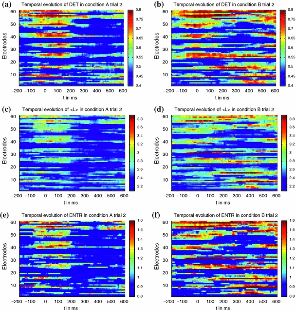
Temporal evolution of chosen RQA measures in condition A and B in a representative trial (trial 2) at all electrode sites. The electrode sites are given in Table 2 in the appendix. In condition B (Fig. 4(b, d, f)) numerous transitions between 300 and 500 ms are found while the control condition A lacks these (Fig.4(a, c, e))

Next, we estimated the 95% confidence interval (CI) of the control condition (99 measurements in total) to which we then compared single trials of the experimental condition B. We did this for the RQA measure RR and preprocessed EEG data. Preprocessing included rereferencing to the mean of the linked mastoids and baseline alignment (300 ms prestimulus). For the RQA measure the experimental condition B could easily be discriminated from the control condition in the relevant time window (Fig. 5). Note that the method is indeed only sensitive to the ERP effect. The measures do not significantly deviate from the control condition apart from the time window which is known to reflect the N400 component (300–500 ms). For the (preprocessed) EEG data it is virtually impossible to distinguish experimental condition (B) from the control condition (A).

Fig. 5.

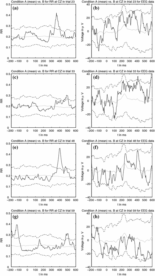
Comparison of single trials (black line) in experimental condition B versus the averaged control condition (grey line) for RR and preprocessed EEG data. The dashed line denotes the 95% CI of the control condition

Statistical analysis

The derived RQA measures were averaged over a small number of trials (10–30) and for every epoch within the relevant time window (−200 to 600 ms relative to the stimulus onset) a pair-wise test was performed.

Instead of the usually applied t-statistic comparison we ran a pairwise Monte-Carlo-Simulation (MCS) (Barnard 1963; Marriott 1979) of a permutation test (Good 2005) since the RQA measures do not necessarily conform to a Gaussian distribution and the requisite for applying a parametric statistic is not met, at least when using sample sizes of only 10–30. For every comparison we ran a total of 1,500 simulations. This is close to the suggested maximum of simulations (Good 2005) and ensures validity of the comparison.

The statistical comparison was performed for n = 30, n = 20 and n = 10 trials in each condition for the measures RR, DET, 〈L 〉, L_max, ENTR and TT. The N400 component can be identified easily by a significant deviation of the measures (Fig. 6). The most remarkable fact is, that even with as few as 10 trials we can detect and statistically prove the existence of the N400 in the data at hand.

Fig. 6.

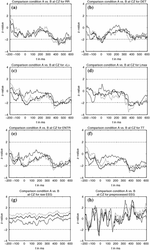
z-value as derived from an MCS of a permutation test for the comparison of condition A and B. The dashed line denotes statistical significance at P = 0.05. The number of trials that entered the analysis were n = 30 (grey line), n = 20 (thick black line) and n = 10 (thin black line)

It could be argued that these results can be achieved with EEG data. In order to have a frame of reference on how effective the traditional analysis is, we applied the exact same testing routine to the EEG data. We tested the preprocessed EEG data (Fig.6h) as well as raw EEG data (Fig. 6g). The raw EEG data could not serve to distinguish the experimental condition at all. With the preprocessed EEG data an overall tendency may be detected, yet the statistical comparison did not only detect the effects in the time window of the N400 but also showed various other significant deviations. Apparently the number of trials is not enough to effectively improve the SNR when using conventional analytical methods. Here the RQA measures are far more effective. In the present data this is most obvious with RR and TT. As the RQA measures were computed from the raw EEG data the direct comparison between Fig. 6a and g further stresses this point.

Note that when using the RQA we lose the notion of polarity and therefore can only use time to identify the effect of interest. This definitely is a drawback of the method since polarity is usually used in characterising ERP components. Therefore the RQA in its current version can only be used for experimental paradigms featuring ERP components that are clearly separated in time. Future versions of the RQA may overcome this problem.

On the other hand, though polarity is a key feature in defining ERP components, it is not necessarily possible to determine the actual polarity of a component. If the polarity of a component cannot be determined on theoretical grounds, grand averages are not able to either. In this case nonlinear methods, such as symbolic dynamics, can provide valuable additional information (beim Graben and Frisch 2004). The various RQA measures defined may possibly also provide such information.

Discussion

We presented an alternative version of RQA and successfully applied it to electrophysiological data recorded in a language processing experiment. The results show that the proposed method can enrich contemporary ERP research, since it poses virtually no restriction on the EEG data at hand and requires no data preprocessing. We were able to find well known correlates of language processing, the N400, in raw EEG data. Furthermore we did so with a number of measurements that is far smaller than the one needed for conventional analysis.

It could be argued that the dataset we investigated is too small, but we think our approach is justified because this article is to be seen as a proof of concept. While in this article we focussed on the methodological part of our research a forthcoming article will be directed at the knowledge about cognitive processes which can be obtained by applying the method proposed.

Further improvement of the method and a tailor-made version of resampling statistics may allow for a focus on the analysis of single trials. Though this is contrary to the widely held opinion that a rather large number of EEG measurements is required in ERP research, we could show that it is indeed possible to focus on a small number of trials.

Additionally, the introduced method may not only serve as a diagnostic tool. Theoretical works on RPs and RQA (see Marwan et al. 2007; and references therein) allow for interpreting the information obtained from (order patterns) RPs within the framework of system theory and system dynamics. As shown above (Fig. 6) the RQA measures in general detected the effect of interest. Yet a certain variation within the measures is visible. As different RQA measures are sensitive to different aspects of the underlying dynamical system, it should be possible to characterise different (language related) ERP components with respect to system dynamics. Further work is required here to shed more light on this aspect of language processing in special and human cognition in general.

Appendix

Electrode sites

Table 2.

Electrode sites used in the language processing experiment (cf. Fig. 4)

#	Electrode	#	Electrode	#	Electrode	#	Electrode	#	Electrode
1	A1	14	F3	27	FT8	40	CPZ	53	P10
2	A2	15	FZ	28	FT10	41	CP4	54	PO7
3	FPZ	16	F4	29	T7	42	CP6	55	PO3
4	FP1	17	F6	30	C5	43	TP8	56	POZ
5	FP2	18	F8	31	C3	44	TP10	57	PO4
6	AF7	19	F10	32	CZ	45	P9	58	PO8
7	AF3	20	FT9	33	C4	46	P7	59	O2
8	AFZ	21	FT7	34	C6	47	P5	60	O1
9	AF4	22	FC5	35	T8	48	P3	61	OZ
10	AF8	23	FC3	36	TP9	49	PZ
11	F9	24	FCZ	37	TP7	50	P4
12	F7	25	FC4	38	CP5	51	P6
13	F5	26	FC6	39	CP3	52	P8

The positions of the electrodes are in accordance with the international 10–20 system (Sharbrough et al. 1991)

References

- Allefeld C, Frisch S, Schlesewsky M (2005) Detection of early cognitive processing by event-related phase synchronization analysis. Neuroreport 16(1):13–16 [DOI] [PubMed]
- Allefeld C, Kurths J (2004) An approach to multivariate phase synchronization analysis and its application to event-related potentials. Int J Bifurcat Chaos 14(2):417–426 [DOI]
- Bandt C, Pompe B (2002) Permutation entropy—a complexity measure for time series. Phys Rev Lett 88:174102 [DOI] [PubMed]
- Barnard G (1963) Discussion of a paper by MS Bartlett. J R Stat Soc Ser B (Stat Methodol) 28:295
- beim Graben P, Frisch S (2004) Is it positive or negative? On determining ERP components. IEEE Trans Biomed Eng 51(8):1374–1382 [DOI] [PubMed]
- beim Graben P, Jurish B, Saddy JD, Frisch S (2004) Language processing by dynamical systems. Int J Bifurcat Chaos 14(2):599–622 [DOI]
- beim Graben P, Saddy JD, Schlesewsky M, Kurths J (2000) Symbolic dynamics of event-related brain potentials. Phys Rev E 62(4):5518–5541 [DOI] [PubMed]
- Cao Y, Tung W, Gao JB, Protopopescu VA, Hively LM (2004) Detecting dynamical changes in time series using the permutation entropy. Phys Rev E 70:046217 [DOI] [PubMed]
- Donchin E, Ritter W, McCallum C (1978) Cognitive psychophysiology: the endogenous components of the ERP. In: Callaway E, Tueting P, Koslow S (eds) Event-related potentials in man. Academic Press, New York, pp 349–441
- Eckmann JP, Kamphorst SO, Ruelle D (1987) Recurrence plots of dynamical systems. Europhys Lett 5:973–977 [DOI]
- Friederici AD (2002) Towards a neural basis of auditory sentence processing. Trends Cogn Sci 6(2):78–84 [DOI] [PubMed]
- Good P (2005) Permutation, parametric and bootstrap tests of hypotheses. Springer Series in Statistics, Springer Verlag
- Groth A (2005) Visualization of coupling in time series by order recurrence plots. Phys Rev E 72(4):046220 [DOI] [PubMed]
- Kandel E, Schwartz J, Jessel T (eds) (1995) Essentials of neural sciences and behavior. Appelton & Lange, East Norwalk, Conneticut
- Kennel MB, Brown R, Abarbanel H (1992) Determining embedding dimension for phase-space reconstruction using a geometrical construction. Phys Rev Lett A 45:3403–3411 [DOI] [PubMed]
- Kutas M, Hillyard S (1980) Reading senseless sentences: brain potentials reflect semantic incongruity. Science 207:203–204 [DOI] [PubMed]
- Kutas M, van Petten C (1994) Psycholinguistics electrified: event-related potential investigations. In: Gensbacher MA (eds) Handbook of psycholinguistics. Academic Press, San Diego, CA, pp 83–143
- Marriott F (1979) Barnard’s monte carlo tests: how many simulations. J R Stat Soc Ser C Appl Stat 28:75–77
- Marwan N, Meinke A (2004) Extended recurrence plot analysis and its application to ERP data. Int J Bifurcat Chaos 14(2):761–771 [DOI]
- Marwan N, Romano MC, Thiel M, Kurths J (2007) Recurrence plots for the analysis of complex systems. Phys Rep 438:237–329 [DOI]
- Marwan N, Wessel N, Meyerfeldt U, Schirdewan A, Kurths J (2002) Recurrence plot based measures of complexity and its application to heart rate variability data. Phys Rev E 66(2):026702 [DOI] [PubMed]
- Poincaré J (1890) Sur le probléme des trois corps et les équations de la dynamic. Acta Math 13:1–270
- Roulston MS (1999) Estimating the errors on measured entropy and mutual information. Physica D 125:285–294
- Sharbrough F, Chatrian G, Lesser R, Lüders H, Nuwer M, Picton T (1991) American electroencephalographic society guideline for standard electrode positions nomenclature. J Clin Neurophysiol 8:200–202 [PubMed]
- Takens F (1981) Detecting strange attractors in turbulence. Lecture notes in mathematics. Springer, Berlin, pp 366–387
- Trulla LL, Giuliani A, Zbilut JP, Webber Jr CL (1996) Recurrence quantification analysis of the logistic equation with transients. Phys Lett A 223(4):255–260 [DOI]