

Abstract
The objective was to determine whether discrepancies between husbands’ and wives’ past year heavy drinking predicted decreased marital satisfaction over time. Participants were recruited at the time they applied for their marriage licenses (N= 634). Couples completed questionnaires about their alcohol use and marital satisfaction at the time of marriage, and again at their first and second anniversaries. Generalized estimating equation models were used to evaluate the association between discrepancies in husbands’ and wives’ heavy drinking in the year prior to marriage and marital satisfaction at the first wedding anniversary and the association between discrepancies in heavy alcohol use in the first year of marriage and marital satisfaction at the second wedding anniversary. In these prospective time-lagged analyses, discrepancies in husbands’ and wives’ heavy drinking predicted decreased marital satisfaction over time while controlling for heavy drinking. Over time, these couples may be at greater risk for decreased marital functioning that may lead to relationship dissolution.
Keywords: marital satisfaction, discrepancies, alcohol use
Marital relationships are often comprised of individuals who share similar backgrounds, values, beliefs, and behaviors. Houts, Robins, and Huston (1996) examined similarity among newly married couples and found that individuals were more closely matched with respect to preferences for leisure activities and for division of household responsibilities than would be expected by chance. In a cross-national study of partner similarity, Price and Vandenberg (1980) found spousal similarity with respect to social variables such as food choices and leisure activities, but also with respect to personality related variables, such as trust, compulsiveness, and social conformity. Spousal similarity has also been demonstrated with respect to psychological disorders, including affective disorder (Galbaud du Fort, Bland, Newman, & Boothroyd, 1998) and antisocial personality (Krueger, Moffitt, Caspi, Bleske, & Silva, 1998).
Although it is not entirely clear whether this similarity is a result of an assortative mating process, a socialization or causation process, or some combination of both, compatibility theories argue that spouses who are quite dissimilar are at risk for marital problems (Kurdek, 1991). This conceptual approach suggests that “….large differences between partners on individual-difference variables … are risk factors for relationship instability” (pages 222-223, Kurdek, 1993). In fact, there is considerable evidence that does suggest that this similarity is associated with marital satisfaction. For example, couples who held similar views as to who should do certain household tasks reported less conflict and less negativity (Houts et al., 1996). In another study of marital relationships, Weisfeld and colleagues (1992) found that couples who were more similar across a variety of domains (e.g., level of education, health, attractiveness) reported significantly higher levels of marital satisfaction. Similarly, stable marriages are often characterized by partner similarity. For example, Levine and Hennessy (1990) found that couples in stable marriages were more likely to report similarity on a variety of personality traits (degree of conservatism, suspiciousness, and concreteness of thinking), compared to those in unstable marriages (marriages that ultimately ended in separation). Concordance for some psychiatric disorders has also been shown to be related to higher marital satisfaction. In a study examining marital quality and anxiety, couples concordant for phobias reported better marital quality compared to couples with only a phobic husband (McLeod, 1994).
Although most of the research focused on similarity and marital satisfaction has been cross-sectional, there is one study that found longitudinal support for this association. Kurdek (1993) followed couples from their first year through their fifth year of marriage. Couples in stable marriages (i.e., those that did not dissolve by the fifth anniversary) were compared to couples who separated or divorced on a variety of variables including personality, beliefs about relationships, marital satisfaction, and motives for being married. Spouses from marriages that dissolved by the end of the study had larger differences on conscientiousness, dysfunctional beliefs about the marriage, the value of the attachment, and motives for being married, compared to stable marriages.
Recent research has extended the examination of spouse similarity to the domain of substance use. As was the case for a variety of traits and behaviors, similarities in substance use have also been noted among married couples. Yamaguchi and Kandel (1993) examined drug use in 545 pairs of couples and found significant concordance for drug use. In another longitudinal study of substance use over the transition to marriage, a high concordance of marijuana use was found among couples from the year before marriage to the couple’s second anniversary (Leonard & Homish, 2005). This similarity also holds true for use of tobacco and alcohol (Homish & Leonard, 2005; Sutton, 1993). For instance, Sutton (1993) found significant correlations in tobacco use among engaged couples, newlyweds, and couples married over five years. Leonard and colleagues (Leonard & Das Eiden, 1999; Leonard & Mudar, 2003) considered spousal similarity for alcohol use in married couples and found significant correlations for average daily volume of alcohol, frequency of heavy drinking, and frequency of intoxication among couples in the year prior to marriage and the year after marriage. Others have also found concordance for alcohol use among married couples (e.g., McLeod, 1993; Windle, 1997).
In accord with compatibility theory, similarity of substance use between husbands and wives may be associated with better overall marital functioning compared to couples whose substance use is dissimilar. Roberts and Leonard (1998) considered the relation between types of “drinking partnerships” and marital functioning. Drinking partnerships were defined as the similarity, or lack thereof, of drinking patterns between husbands and wives. Couples with discordant drinking patterns reported poorer marital functioning. Mudar, Leonard, and Soltysinski (2001) assessed marital functioning in a community sample of newlyweds to examine whether the configuration of partners’ drinking patterns was related to marital functioning. The drinking patterns consisted of four groups, one concordant for use, one concordant for nonuse, and the two discordant groups (husband only use, wife only use). Additionally, a variety of levels of consumption were also considered (any alcohol use, regular drinking, heavier drinking, and frequent intoxication). For heavier drinking and frequent intoxication, there were no significant differences in marital quality between the two concordant groups (neither engage in behavior vs. both do) and no differences between the two discordant groups (husband only vs. wife only). However, discordant couples had significantly lower marital quality compared to couples where neither partner used alcohol at these levels and compared to couples where both partners consumed at these levels. The latter finding suggests that the mutual patterning of drinking (i.e., concordance of drinking behaviors vs. discordant drinking behaviors) is a key element involved in the relation between alcohol consumption and marital functioning, and may be more important that the level of drinking by either partner. Similarly, Leadley, Clark, & Caetano (2000) used data from the Ninth National Alcohol Survey and found that discrepant alcohol use was related to relationship distress and incidence of violence. However, both of these studies relied on cross-sectional analyses, and did not examine longitudinal effects.
The goal of this longitudinal study was to extend our previous, cross-sectional work (Mudar et al., 2001) that found that discrepant alcohol use in newlyweds was associated with lower levels of marital satisfaction. In particular, we focused on discrepancies in the frequency of heavy alcohol consumption because our previous findings suggested that discrepancies with respect to regular, nonheavy consumption were not associated with marital satisfaction cross-sectionally (Mudar et al., 2001). We hypothesized that the discrepancy between husbands and wives would be related to decreased marital satisfaction for both husbands and wives over the first two years of marriage, and that this effect would be independent of heavy drinking for the husband or wife.
Methods
Participants
Participants for this report were involved in a longitudinal study of marriage and alcohol involvement. All participants were at least 18 years old, spoke English, and were literate. Couples were ineligible for the study if they had been previously married. These analyses are based on 634 couples. At the initial assessment, the average age of the men [mean (SD)] was 28.7 (6.3) years and the average of the women was 26.8 (5.8) years. The majority of the men and women in the sample were European American (husbands: 59%; wives: 62%). About one-third of the sample was African American (husbands: 33%; wives: 31%). The sample also included small percentages (less than 5%) of Hispanic, Asian, and Native American participants. A large proportion of husbands and wives had at least some college education (husbands: 64%; wives: 69%) and most were employed at least part-time (husbands: 89%; wives 75%). Consistent with other recent studies of newly married couples (e.g., Chadiha, Veroff, & Leber, 1998; Crohan & Veroff, 1989; Orbuch & Veroff, 2002; Tallman, Burke, & Gecas, 1998), many of the couples were parents at the time of marriage (38% of the husbands and 43% of the wives) and were living together prior to marriage (70%). The Institutional Review Board of the State University of New York at Buffalo approved the research protocol.
Procedures
After applying for a marriage license, couples were recruited for a 5-10 minute paid ($10) interview. The interview covered demographic factors (e.g. race, education, age), family and relationship factors (e.g. number of children, length of engagement), and substance use questions (e.g. tobacco use, average alcohol consumption, times intoxicated in the past year). This interview took place at the city hall in an area away from other individuals. Recruitment occurred over a 3 year period from 1996-1999. For interested individuals who did not have time to complete this interview, a telephone interview was conducted later that day or the next day (N = 62). Less than 8% of individuals approached declined to participate. We interviewed 970 eligible couples (Figure 1).
Figure 1.
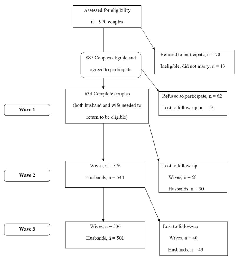
Participation Rates
Complete details of the recruitment process can be found elsewhere (Leonard & Mudar, 2000; Leonard & Mudar, 2003), but briefly, couples who agreed to participate were given identical questionnaires to complete at home and asked to return in separate postage paid envelopes (Wave 1 Assessment). Participants were asked not to discuss their responses with their partners. Each spouse received $40 for their participation. Only 7% of eligible couples refused to participate. Those who agreed to participate, compared to those who did not, were more likely to have lower incomes (p < .01) and the women were more likely to have children (p < .01). No other differences were identified. Of the 887 eligible couples who agreed to participate (13 of the original 900 did not marry), data were collected from both spouses for 634 couples (71.4%). The 634 couples are the basis for this report. Couples who returned the questionnaires were more likely to be living together compared to couples who did not return the questionnaires (70% vs. 62%; p < .05) and more likely to be European American (p < .05). No other sociodemographic differences existed between the couples who responded compared to those who did not. Average past year alcohol consumption did not differ between couples that returned the questionnaires and those who did not. Husbands in non-respondent couples consumed 6 or more drinks (p < .05) or were intoxicated in the past year (p < .05) more often than husbands who completed the questionnaire; however, these differences were small. These items were measured on a 9-point scale (0, not in the past year, to 8, everyday in the past year). The mean difference between respondent husbands and non-respondent husbands on the frequency of drinking 6 or more drinks on an occasion was 0.29 (effect size = 0.17), with non-respondents drinking 6 or more drinks on an occasion slightly more often. Similarly, the difference for frequency of intoxication was 0.24 (effect size = 0.16), with non-responders reporting a greater frequency of drinking to intoxication.
At the couples’ first and second anniversaries (Waves 2 and 3), they were mailed questionnaires similar to those they received at the first assessments. As with the first assessment, they were asked to complete the forms and return them in the postage paid envelopes. Each spouse received $40 for their participation at each wave. Wives who did not participate in the second and third assessments were slightly younger (p < .05) and somewhat less educated than other wives (p <.05). Husbands who did not participate were less likely to be European American compared to the other husbands (p < .05). Wave 1 marital satisfaction for both husbands and wives did not differ for those who were lost to follow-up compared to those who completed the questionnaires.
Measures
Heavy Drinking Discrepancy
Frequency of intoxication was assessed on a 9-point scale that ranged from “didn’t get drunk last year” (coded 0) to “everyday” (coded 8). The frequency of drinking 6 or more drinks on an occasion was also assessed using the same 9-point scale.1 In preliminary analyses, we found these two variables to be correlated (average correlation for husbands: .75, p < .001; average correlation for wives: .69, p < .001); however, answers for frequency of intoxication and frequency of drinking 6 or more drinks were identical for less than 50% of husband and wives. Approximately 23% of husbands drank 6 or more drinks more often than they were intoxicated and 13% reported frequency of intoxication more often than they reported drinking 6 or more drinks. Among wives, 12% of wives drank 6 or more drinks more often than they reported frequency of intoxication and 21% reported a greater frequency of intoxication compared to how often they drank 6 or more drinks. In a repeated measures ANOVA, the interaction between member (husband-wife) and item (intoxication vs. 6 plus) was significant indicating gender difference in the way they answered the two items. The interaction suggested that men more frequently reported drinking 6 or more drinks on an occasion and wives more frequency reported drinking to intoxication. Because of this difference, we defined heavy drinking as the maximum of these two responses.
To test the reliability of our single item measures of frequency of intoxication and frequency of drinking 6 or more drinks, correlations were examined between Wave 1 responses to these items and participants’ responses to these items at the screening interview at city hall. These two assessments differed in type (interview versus questionnaire), context (city hall vs. at home), and time (approximately 1-2 months between city hall interview and receipt of questionnaires). Nonetheless, among husbands, frequency of 6 or more drinks reported at the screening was significantly correlated with their response to this item at Wave 1 (r= .57, p <.01) as well as the correlation for frequency of intoxication (r = .68, p <.01). The comparable correlations for the wives were .65 (p < .01) and .44 (p < .01). Additionally, we examined the correlations between participants’ response to these items on the questionnaire and their partners’ report of their behavior. For both the frequency of intoxication and the frequency of drinking 6 or more drinks, participants report was significantly correlated with their partners’ reporting of their behavior (correlations range from .51 to .65 and all were significant at p < .01).
For each wave, the discrepancies between husbands’ and wives’ reports of their heavy were calculated by subtracting wives’ responses from their husbands’ responses. The drinking discrepancy variable was modeled in the regression models in two ways, as a time-varying linear predictor and as a time-varying quadratic predictor. The linear variable allowed for the examination of whether husbands were heavier drinkers than wives and whether this was related to marital satisfaction. The quadratic predictor captured discrepancies between partners regardless of who drank more.2
Relationship Quality
At each assessment, marital quality was assessed with the Marital Adjustment Test (MAT, Locke & Wallace, 1959). The MAT consists of 15 total items. One item measures overall degree of happiness (7 response choices from very happy to perfectly happy). Eight other items ask participants to rate how often they agree with their partner on a variety of topics (e.g., family finances, ways of dealing with in-laws, matters of recreation, etc.). These items are scored on a 6-point scale rated from always agree to always disagree. An additional 6 questions asks participants to report on other aspects of the relationship. These questions each have a varying number of possible responses from 2 to 4 possible outcomes (e.g., do you confide in your mate, 3 response choices; ever wish you didn’t get married, 4 response choices). This instrument measures overall relationship quality. Higher scores indicated greater relationship quality (range: 2-158). The MAT had a high reliability across all waves of the study (range of coefficient alpha’s across the three waves for the men: .81-.88; among women, the range of coefficient alpha’s: .80-.91). A score of less than or equal to 100 is usually considered to reflect clinically significant marital distress.
Demographic Factors
At the initial in-person interview, each spouse reported their age, race/ethnicity, income, highest level of education obtained, employment status, number of children they had prior to the current marriage, and the number of months cohabitating.
Analysis
Descriptive statistics were used to cross-sectionally characterize husbands’ and wives’ marital satisfaction, frequency of heavy drinking, and the discrepancy between husbands’ heavy drinking and wives’ heavy drinking. Paired t-tests compared husbands and wives on these variables at each time point. Spearman correlations were used to assess the relation between heavy drinking, discrepancy of heavy drinking, and marital satisfaction at each wave. To examine the association between the discrepancy in heavy drinking between wives and husbands at one time point and marital satisfaction at subsequent assessments, we used Generalized Estimating Equations (GEE) (Zeger & Liang, 1986; Zeger, Liang, & Albert, 1988). GEE models are used to analyze data from longitudinal designs with discrete or continuous outcomes (Zeger et al., 1988). Because longitudinal datasets contain repeated observations of the same participants over time, the data is often correlated, thus requiring more specialized analytic tools. GEE models can be used to assess the longitudinal relationship between several time-varying and time-invariant predictors and the outcome variable (Twisk, 2004). In addition to appropriately handling correlated data structures, GEE models are also useful for dealing with cases with missing observations. For many other analysis (e.g., repeated measures ANOVA’s), participants who do not provide data for each assessment are considered missing; however; GEE modeling allows participants with only information from one assessment to be included in the analyses (Twisk, 2004). The nature of the missing data, however, should be missing at random. In the current work, Wave 1 marital satisfaction for both husbands and wives did not differ for those who were lost to follow-up compared to those who completed the questionnaires.
For the current report, two GEE models were analyzed. The first model focused on husbands’ marital satisfaction and the second model focused on wives’ marital satisfaction. The models were analyzed with Stata (Version 8, StataCorp, 2003b). The drinking discrepancy was modeled as a time varying predictor and the outcome variable, marital satisfaction, was estimated as a continuous variable. Because the outcome variable is a continuous, normally distributed variable, the GEE models were estimated with a Gaussian Family and Identity Link. An autoregressive correlation structure with a lag of 1 was specified along with robust standard errors. The robust standard errors are used so that if the nature of the correlation structure is not correctly specified, the standard errors will still be valid (StataCorp, 2003a). A lagged design was used so that Wave 1 alcohol discrepancy can be used to predict Wave 2 marital satisfaction and Wave 2 alcohol discrepancy can be use to predict Wave 3 marital satisfaction. Prior wave heavy drinking was entered as a time varying covariate. Baseline (Wave 1) sociodemographic variables were entered as time-invariant covariates.
Results
At the first assessment, wives’ average score on the Marital Adjustment Test was 120.5 (SD= 20.1) and husbands’ average score was 117.9 (SD= 20.8). The scores are similar to other samples of first-time married newlyweds’ marital satisfaction scores (e.g., Carrere, Buehlman, Gottman, Coan, & Ruckstuhl, 2000). The difference between husbands and wives’ marital satisfaction at Wave 1 was statistically significant; however, at Waves 2 and 3, there were no significant differences between husbands’ and wives’ marital satisfaction (Table 1). Husbands’ and wives’ marital satisfaction significantly decreased at each wave (for husbands, the difference between Waves 1 and 2 was significant at p < .001, for Waves 2 and 3, p < .05; for wives, each difference was significant at p < .001). At each wave, husbands reported significantly higher levels of heavy drinking (both frequency of intoxication and frequency of drinking 6 or more drinks on an occasion). When considering the discrepancy between husbands’ and wives’ heavy drinking (defined as the maximum of the frequency of intoxication and frequency of drinking 6 or more drinks on an occasion), the greatest discrepancy occurred at Wave 2 (mean [SD], 1.13 [1.43]), followed by Wave 3 (1.07 [1.41]), and Wave 1 (1.10 [1.44]). The differences in discrepancies over time were not statistically significant.
Table 1.
Descriptive Statistics
| Husband Variables | Wife Variables | |||||
|---|---|---|---|---|---|---|
| Wave 1 | Wave 2 | Wave 3 | Wave 1 | Wave 2 | Wave 3 | |
| Marital Satisfaction (mean, st. dev) | 117.9** (20.8) | 108.6 (28.2) | 105.8 (30.2) | 120.5 (20.1) | 109.1 (29.5) | 105.1 (33.4) |
| Frequency of Intoxication (mean, st. dev) | 2.2*** (1.4) | 2.1*** (1.4) | 2.0*** (1.2) | 1.8 (1.0) | 1.7 (1.0) | 1.6 (1.0) |
| Frequency of 6 or more drinks (mean, st. dev) | 2.4*** (1.7) | 2.3*** (1.7) | 2.2*** (1.6) | 1.7 (1.2) | 1.6 (1.2) | 1.5 (1.2) |
| Frequency of Heavy Drinking (%) | ||||||
| Weekly or more | 15.0% | 13.0% | 11.4% | 5.4% | 4.5% | 4.6% |
| 1+ times per month | 19.7% | 20.2% | 18.9% | 11.7% | 8.9% | 7.4% |
| 1+ times per year | 35.0% | 33.0% | 35.1% | 41.6% | 37.6% | 36.6% |
| None in the past year | 30.3% | 33.8% | 34.6% | 41.3% | 49.0% | 51.4% |
p < .001;
p < .01, testing differences between husband and wife scores at each Wave
Notes: Marital Satisfaction was assessed with Marital Adjustment Scale (range 2-158). Higher scores indicate greater marital satisfaction. Frequency of intoxication and frequency of 6 or more drinks were assessed on a 9-point scale (0-8) with higher scores indicating greater frequency. Heavy Drinking was defined as the maximum of frequency of intoxication and frequency of drinking 6 or more drinks.
To examine the cross-sectional association between heavy drinking and marital satisfaction, a series of Spearman correlations were examined. At each wave, husbands’ heavy drinking was negatively correlated with husbands’ marital satisfaction (Table 2). Husbands’ heavy drinking was also significantly negatively correlated with wives’ marital satisfaction at all waves. Wives’ heavy drinking was significantly negatively correlated with marital satisfaction among wives at all waves. Wives’ heavy drinking was significantly negatively correlated with husbands’ marital satisfaction, but only at Wave 3. The second set of correlations assessed the relation between level of discrepancy between husbands’ and wives’ heavy drinking and marital satisfaction. The discrepancy was considered as both a linear variable and a quadratic variable. A stronger relation was found between the quadratic discrepancy term and both husbands’ and wives’ marital satisfaction at all waves compared to the linear discrepancy term (Table 2). The final set of correlations examined the relation between the drinking discrepancy variables and marital satisfaction while controlling for heavy drinking. These partial correlations were very similar to the simple correlations in Table 2 and are not presented here.
Table 2.
Cross-sectional Spearman Correlations between Heavy Drinking, Discrepancy and Marital Satisfaction
| Husbands’ Marital Satisfaction | Wives’ Marital Satisfaction | |||||
|---|---|---|---|---|---|---|
| Wave 1 | Wave 2 | Wave 3 | Wave 1 | Wave 2 | Wave 3 | |
| Husband Heavy Drinking | -.06* | -.13** | -.16** | -.06 | -.10* | -.11* |
| Wife Heavy Drinking | -.04 | -.02 | -.13** | -.08 | -.09* | -.15** |
| Drinking Discrepancy (linear) | -.06 | -.13** | -.06 | -.01 | -.06 | .01 |
| Drinking Discrepancy (quadratic) | -.09* | -.19** | -.17** | -.10* | -.17** | -.16** |
p < .01;
p < .05;
Heavy drinking = maximum of Frequency of Intoxication and Frequency of drinking 6 or more drinks on an occasion; Discrepancy = the discrepancy between husbands’ and wives’ frequency of heavy drinking
The longitudinal association of discrepancies between husbands’ and wives’ heavy drinking and marital association were examined with two sets of Generalized Estimating Equation Models. The dependent variable for the first model was husbands’ marital satisfaction and wives’ marital satisfaction was the outcome for the second model. The discrepancy between husbands’ and wives’ frequency of heavy drinking was modeled in two ways, as a linear term and as a quadratic term. These terms were modeled as time-varying predictors and the prior wave discrepancy was used to predict changes in marital satisfaction. Both the linear and quadratic terms were entered simultaneously in the models. In all models, baseline demographic and background variables (age, income, education, race, months living together prior to marriage and whether or not the participant had a child prior to this marriage) and heavy drinking (maximum of the frequency of intoxication and the frequency of drinking 6 or more drinks on an occasion) were entered as covariates.3 Prior wave heavy drinking was modeled as a time-varying covariate.
Husbands’ marital satisfaction was the outcome variable in the first GEE model. Husbands’ prior wave frequency of heavy drinking was not associated with husbands’ marital satisfaction at subsequent waves (β = -0.82, 95% confidence interval [CI]: -2.21, 0.82, NS, Table 3). Baseline (Wave 1) income was significantly associated with husbands’ marital satisfaction (β = 1.65, 95% CI: 0.46, 2.84, p < .01). None of the other background or demographic variables was significantly associated with husbands’ marital satisfaction. After controlling for husbands’ heavy drinking and husbands’ background and demographic factors, the discrepancy between husbands’ and wives’ heavy drinking in the previous wave was not longitudinally predictive of husbands’ marital satisfaction when the drinking discrepancy was modeled as a linear predictor (β = 0.42, 95% CI: -.70, 1.54, NS). However, when the discrepancies were modeled as a quadratic term, a greater discrepancy between husbands’ and wives’ frequency of heavy drinking was longitudinally predictive of decreased levels of marital satisfaction (β = -0.49, 95% CI: -0.72, -0.25, p < .001, Figure 2).
Table 3.
Longitudinal Association between Discrepancies and Husbands’ Marital Satisfaction
| Predictor | Regression Coefficient | Robust Standard Error | 95% Confidence Interval | |
|---|---|---|---|---|
| Husband Heavy Drinking | -.82 | .71 | -2.21 | .57 |
| Husband Income | 1.65** | .61 | .46 | 2.84 |
| Husband Age | .09 | .17 | -.24 | .42 |
| Husband a Parent Prior to this Marriage | -.26 | 2.11 | -4.39 | 3.89 |
| Husband Education | 1.23 | 1.94 | -2.57 | 5.05 |
| Husband Race/Ethnicity | 2.03 | 2.00 | -1.88 | 5.95 |
| Months Living Together Prior to this Marriage | .03 | .03 | -.03 | .09 |
| Linear Drinking Discrepancy | .42 | .57 | -.70 | 1.54 |
| Quadratic Drinking Discrepancy | -.49*** | .12 | -.72 | -.25 |
p < .01;
p < .001
Figure 2.

Husband and Wife Marital Satisfaction and Alcohol Discrepancies
Footnote: The curves represent the fitted values with the 95% confidence interval from each model. Positive alcohol discrepancies indicate greater levels of husband drinking compared to wife drinking, while negative discrepancies indicate greater levels of wife drinking compared to husband drinking.
In the second model focused on wives’ marital satisfaction, more frequent heavy drinking among wives was associated, at a trend level, with decreased wives’ marital satisfaction at subsequent waves (β = -1.62, 95% CI:-3.36, 0.11, p < .07, Table 4). Baseline (Wave 1) income was positively related to wives’ marital satisfaction (β = 2.75, 95% CI: 1.39-4.11, p < .001). None of the wives’ other background or demographic variables was associated with wives’ marital satisfaction. In this model, a similar pattern was observed with regard to the discrepancy between husbands’ and wives’ heavy drinking as found in the husband model. That is, prior wave discrepancies in alcohol use were not longitudinally predictive of wives’ marital satisfaction when they were modeled as a linear term (β = 0.16, 95% CI: -1.20, 1.52, NS); however, prior wave quadratic drinking discrepancy was longitudinally predictive of wives’ marital satisfaction, with greater discrepancies between husbands’ and wives’ frequency of heavy drinking related to lower marital satisfaction among wives at subsequent waves (β = -0.46, 95 % CI: -0.77, -0.14, p < .01, Figure 2).4
Table 4.
Longitudinal Association between Discrepancies and Wives’ Marital Satisfaction
| Predictor | Regression Coefficient | Robust Standard Error | 95% Confidence Interval | |
|---|---|---|---|---|
| Wife Heavy Drinking | -1.62ˆ | .89 | -3.36 | .11 |
| Wife Income | 2.75*** | .69 | 1.39 | 4.11 |
| Wife Age | .23 | .18 | -.11 | .58 |
| Wife a Parent Prior to this Marriage | 2.52 | 2.25 | -1.87 | 6.93 |
| Wife Education | 2.44 | 2.02 | -1.87 | 6.76 |
| Wife Race/Ethnicity | .93 | 2.17 | -3.33 | 5.19 |
| Months Living Together Prior to this Marriage | .01 | .03 | -.06 | .07 |
| Linear Drinking Discrepancy | .16 | .69 | -1.20 | 1.52 |
| Quadratic Drinking Discrepancy | -.46** | .16 | -.77 | -.14 |
p < .07;
p < .05,
p < .01;
p < .001
Discussion
Previous cross-sectional work has shown that couples who reported a discrepant pattern of alcohol use at the time of marriage had lower levels of marital satisfaction compared to couples who reported that both partners used, or that neither partner used (Mudar et al., 2001). This was true for heavier drinking, frequency of intoxication, and for drug use. The current report provides longitudinal support that discrepant patterns of alcohol use are predictive of poorer marital satisfaction. This significant association between discrepant drinking and decreased marital satisfaction was observed for both men’s and women’s satisfaction. It is also important to recognize that this effect was independent of frequent heavy drinking by the participant, which was statistically controlled in the analyses. Moreover, in previous analyses of this dataset, Kearns-Bodkin and Leonard (2005) examined the longitudinal relationship between partner drinking and marital satisfaction with a latent growth modeling approach. While there was evidence that changes in partner drinking and changes in marital satisfaction were correlated, there was no evidence that partner drinking predicted subsequent changes in marital satisfaction for either husbands or wives. Overall, these results suggest that within a general population sample, discrepant drinking patterns between the partners, rather than simply heavy drinking by one partner, are most strongly and longitudinally associated with marital satisfaction.
There are several possible reasons for the effects that we found in the current report. Discrepancies between husbands’ and wives’ heavy drinking may suggest dissimilarity in the couples in other respects, which in turn, could be the reason for the association between discrepant drinking and decreased marital satisfaction. It is important to note, however, that discrepancies were related to marital satisfaction when modeled as a quadratic factor. Thus, regardless of who was the heavier drinker, it was the differences between husband and wife heavy drinking that was related to marital satisfaction. If the linear term had been significant (which it was not in the current report), this would have indicated that the relation between drinking discrepancy and marital satisfaction was dependent on who (husband vs. wife) was the heavier drinker. Compatibility theories suggest that couples who are more similar are more likely to have more satisfying marriages (Levinger & Rands, 1985). Weisfeld and colleagues (1992) assessed marital satisfaction and similarities across a wide range of characteristics and found support for the hypothesis that more similar couples would have greater marital satisfaction. Therefore, the discrepancies in heavy drinking between husbands and wives may be indicative of dissimilar values or attitudes, or different expectations concerning appropriate behavior in marriage.
Another possible explanation of the association between alcohol discrepancies and marital functioning may that discrepancies in drinking behavior may be indicative of decreased marital interaction. For example, Fals-Stewart and colleagues (1999) suggested that for “…some dual drug-abusing couples, drug use becomes positively associated with relationship satisfaction, perhaps because substance use becomes an important shared recreational activity” (page 21). Therefore, couples with dissimilar patterns of substance use may be less likely to spend time together, and, this decreased social interaction may lead to poorer marital functioning. Research on marital satisfaction and leisure activities suggests that couples who are involved in activities apart from their spouses are more likely to report lower levels of marital satisfaction (e.g., Holman & Jacquart, 1988).
Although the mechanism responsible for the association between alcohol discrepancy and marital satisfaction is not clear, this work is consistent with previous work that has found alcohol discrepancies to be related to aversive marital behaviors. Quigley and Leonard (2000) examined the relation between husbands’ and wives’ patterns of alcohol consumption and marital aggression over the early marital years. The highest level of husband to wife aggression was found in discordant couples (husband heavy drinker, wife not). Further, husband’s drinking was only predictive of aggression in the next two years when wife’s drinking was also considered. Others have also found that discordant substance use, not substance use per se, was associated with relationship difficulties. For example, Leadley, Clark, and Caetano (2000) found that couples whose alcohol use was discrepant were more likely to have serious relationships difficulties such as alcohol-related arguments and violence.
There are several clinical implications of the findings reported here. First, as individuals develop and experience various events, one individual may change his or her drinking behavior, and a couple may shift from a congruent heavy drinking partnership to a discrepant pattern. The results of this study suggest that such transitional points in drinking may serve as important transitional points for marital functioning, and could provide targeted developmental periods for interventions. For example, the recognition of pregnancy and the birth of a child often lead to reductions in drinking. A couple in which the wife reduced her drinking at this point, but the husband did not could be at an increased risk for decrements in marital satisfaction that go beyond the decrement commonly observed in couples after the birth of a child. Second, the results highlight a potential clinical dilemma in the context of heavy drinking couples in which one partner is involved in alcohol treatment. The current study raises the possibility that successful treatment of one member of a congruent heavy drinking couple may exacerbate marital problems. Given the proven value of behavioral couples therapy for alcohol problems (O=Farrell & Fals-Stewart, 2003), these results provide a further rationale for involving both members of a congruent heavy drinking couple in interventions.
Several limitations need to be considered when evaluating this report. Although we found that the discrepancy between husband’s and wife’s heavy drinking was predictive of decreased marital satisfaction, there are many other factors that may have been involved in the declines in marital satisfaction that we observed. For example, depression (Fincham, Beach, Harold, & Osborne, 1997), the birth of a first child (Hackel & Ruble, 1992), the number of children (Twenge, Campbell, & Foster, 2003), and expectations about marriage (McNulty & Karney, 2004) are just a few factors that have been found to be associated with changes in marital satisfaction. The sample for the current report was comprised of newly married couples involved in their first marriages. Therefore, our findings may not be generalizable to couples who have been married for a longer duration or to couples involved in second marriages. Although our retention rates over time were good, the number of complete eligible couples who returned the time 1 questionnaire was lower than was anticipated; however, differences between the responders and non-responders were quite minimal.
Despite these limitations, we found a significant association between discrepancies in husbands’ and wives’ heavy drinking and later marital satisfaction. The use of a large, longitudinal cohort of newly married couples allowed us to extend previous cross-sectional work that found the discordant patterns of alcohol use were related to lower levels of marital satisfaction. Future work will need to consider if this trend continues in later years of marriage and identify consequences that may result. For example, it may lead to violence in the relationships and/or marital dissolution. Further, it will be important to identify other factors that are involved in the relation between alcohol use patterns between husbands’ and wives’ and overall marital functioning of the couple.
Acknowledgments
The research for this manuscript was supported by grant R37-AA09922 from the National Institute on Alcohol Abuse and Alcoholism.
Footnotes
The first assessments of this study occurred before it became common for “binge drinking” to be operationally defined as 5 drinks for men on an occasion and 4 drinks for women on an occasion. Although we have added these questions to later waves of the study, the first three assessments that are reported here asked men and women to report the frequency of drinking 6 or more drinks on an occasion.
One could assess discrepancy on the basis of the absolute value of the difference between husband and wife drinking. However, an association between the absolute value of the difference and marital satisfaction could occur if the association only occurred among husbands who drank more than wives, or alternatively, among wives who drank more than husbands. We chose to include both the linear and quadratic terms of the actual discrepancy to assess and control for these possibilities.
We did not include partner drinking as a covariate because discrepant drinking was a linear combination of one’s own and partner’s drinking.
Several additional analyses were conducted to ensure that the observed effects were not artifacts. First, we conducted similar analyses with absolute values of the discrepancy, rather than a quadratic term, and found the same results. To make sure that the results could not be attributed to non discrepant couples who never drank to excess, we omitted such couples from the analyses, and the quadratic effect remained significant, and became numerically larger.
Publisher's Disclaimer: The following manuscript is the final accepted manuscript. It has not been subjected to the final copyediting, fact-checking, and proofreading required for formal publication. It is not the definitive, publisher-authenticated version. The American Psychological Association and its Council of Editors disclaim any responsibility or liabilities for errors or omissions of this manuscript version, any version derived from this manuscript by NIH, or other third parties. The published version is available at http://www.apa.org/journals/ccp/
Contributor Information
Gregory G. Homish, Research Institute on Addictions, University at Buffalo, The State University of New York, 1021 Main Street, Buffalo, NY 14203-1016, Phone 716-887-3306, Fax 716-887-2510, Email: ghomish@ria.buffalo.edu
Kenneth E. Leonard, Research Institute on Addictions, University at Buffalo, The State University of New York And Department of Psychiatry, School of Medicine, University at Buffalo, The State University of New York, 1021 Main Street, Buffalo, NY 14203-1016
References
- Carrere S, Buehlman KT, Gottman JM, Coan JA, Ruckstuhl L. Predicting marital stability and divorce in newlywed couples. Journal of Family Psychology. 2000;14(1):42–58. doi: 10.1037//0893-3200.14.1.42. [DOI] [PubMed] [Google Scholar]
- Chadiha LA, Veroff J, Leber D. Newlywed’s narrative themes: Meaning in the first year of marriage for African American and White couples. Journal of Comparative Family Studies. 1998;29(1):115–130. [Google Scholar]
- Crohan SE, Veroff J. Dimensions of marital well-being among white and black newlyweds. Journal of Marriage & the Family. 1989;51(2):373–383. [Google Scholar]
- Deal JE, Wampler KS, Halverson CF., Jr The importance of similarity in the marital relationship. Fam Process. 1992;31(4):369–382. doi: 10.1111/j.1545-5300.1992.00369.x. [DOI] [PubMed] [Google Scholar]
- Fals-Stewart W, Birchler GR, O’Farrell TJ. Drug-abusing patients and their intimate partners: Dyadic adjustment, relationship stability, and substance use. Journal of Abnormal Psychology February. 1999;108(1):11–23. doi: 10.1037//0021-843x.108.1.11. [DOI] [PubMed] [Google Scholar]
- Fincham FD, Beach SR, Harold GT, Osborne LN. Marital satisfaction and depression: Different causal relationships for men and women? Psychological Science. 1997;8(5):351–357. [Google Scholar]
- Galbaud du Fort G, Bland RC, Newman SC, Boothroyd LJ. Spouse similarity for lifetime psychiatric history in the general population. Psychol Med. 1998;28(4):789–802. doi: 10.1017/s0033291798006795. [DOI] [PubMed] [Google Scholar]
- Hackel LS, Ruble DN. Changes in the marital relationship after the first baby is born: Predicting the impact of expectancy disconfirmation. J Pers Soc Psychol. 1992;62(6):944–957. doi: 10.1037//0022-3514.62.6.944. [DOI] [PubMed] [Google Scholar]
- Holman TB, Jacquart M. Leisure-activity patterns and marital satisfaction: A further test. Journal of Marriage and the Family. 1988;50(1):69–77. [Google Scholar]
- Homish GG, Leonard KE. Spousal influence on smoking behaviors in a US community sample of newly married couples. Social Science & Medicine. 2005;61(12):2557–67. doi: 10.1016/j.socscimed.2005.05.005. [DOI] [PMC free article] [PubMed] [Google Scholar]
- Houts RM, Robins E, Huston TL. Compatibility and the development of premarital relationships. Journal of Marriage & the Family. 1996;58(1):7–20. [Google Scholar]
- Johnson PL, O’Leary KD. Behavioral components of marital satisfaction: An individualized assessment approach. Journal of Consulting & Clinical Psychology. 1996;64(2):417–423. doi: 10.1037//0022-006x.64.2.417. [DOI] [PubMed] [Google Scholar]
- Karney BR, Story LB, Bradbury TN. Marriages in context: Interactions between chronic and acute stress among newlyweds. In: Revenson TA, Kayser K, Bodenmann G, editors. Emerging perspectives on couples’ coping with stress. Washington, DC: American Psychological Association; in press. [Google Scholar]
- Kearns-Bodkin JN, Leonard KE. Alcohol involvement and marital quality in the early years of marriage: A longitudinal growth curve analysis. Alcoholism, Clinical and Experimental Research. 2005;29(12):2123–2134. doi: 10.1097/01.alc.0000191751.62025.77. [DOI] [PubMed] [Google Scholar]
- Krueger RF, Moffitt TE, Caspi A, Bleske A, Silva PA. Assortative mating for antisocial behavior: Developmental and methodological implications. Behav Genet. 1998;28(3):173–186. doi: 10.1023/a:1021419013124. [DOI] [PubMed] [Google Scholar]
- Kurdek LA. Marital stability and changes in marital quality in newly wed couples - a test of the contextual model. J Soc Pers Relat. 1991;8(1):27–48. [Google Scholar]
- Kurdek LA. Predicting marital dissolution - a 5-year prospective longitudinal-study of newlywed couples. J Pers Soc Psychol. 1993;64(2):221–242. [Google Scholar]
- Leadley K, Clark CL, Caetano R. Couples’ drinking patterns, intimate partner violence, and alcohol-related partnership problems. J Subst Abuse. 2000;11(3):253–263. doi: 10.1016/s0899-3289(00)00025-0. [DOI] [PubMed] [Google Scholar]
- Leonard KE, Das Eiden R. Husband’s and wife’s drinking: Unilateral or bilateral influences among newlyweds in a general population sample. J Stud Alcohol Suppl. 1999;13:130–138. doi: 10.15288/jsas.1999.s13.130. [DOI] [PubMed] [Google Scholar]
- Leonard KE, Homish GG. Changes in marijuana use over the transition into marriage. J Drug Issues. 2005;35(2):409–430. doi: 10.1177/002204260503500209. [DOI] [PMC free article] [PubMed] [Google Scholar]
- Leonard KE, Mudar P. Alcohol use in the year before marriage: Alcohol expectancies and peer drinking as proximal influences on husband and wife alcohol involvement. Alcohol Clin Exp Res. 2000;24(11):1666–1679. [PubMed] [Google Scholar]
- Leonard KE, Mudar P. Peer and partner drinking and the transition to marriage: A longitudinal examination of selection and influence processes. Psychol Addict Behav. 2003;17(2):115–125. doi: 10.1037/0893-164x.17.2.115. [DOI] [PubMed] [Google Scholar]
- Levine KS, Hennessy JJ. Personality influences in the stability of early (teen-age) marriage in the united states. Current Psychological Research & Reviews. 1990;9(3):296–303. [Google Scholar]
- Levinger G, Rands M. Compatibility in marriage and other close relationships. In: Ickes WJ, editor. Compatible and incompatible relationships. New York: Springer-Verlag; 1985. pp. 309–331. [Google Scholar]
- Locke HJ, Wallace KM. Short marital-adjustment prediction tests: Their reliability and validity. Marriage and Family Living. 1959;21:251–255. [Google Scholar]
- McLeod JD. Spouse concordance for alcohol dependence and heavy drinking: Evidence from a community sample. Alcohol Clin Exp Res. 1993;17(6):1146–1155. doi: 10.1111/j.1530-0277.1993.tb05220.x. [DOI] [PubMed] [Google Scholar]
- McLeod JD. Anxiety disorders and marital quality. Journal of Abnormal Psychology November. 1994;103(4):767–776. doi: 10.1037//0021-843x.103.4.767. [DOI] [PubMed] [Google Scholar]
- McNulty JK, Karney BR. Positive expectations in the early years of marriage: Should couples expect the best or brace for the worst? J Pers Soc Psychol. 2004;86(5):729–743. doi: 10.1037/0022-3514.86.5.729. [DOI] [PubMed] [Google Scholar]
- Mudar PJ, Leonard KE, Soltysinski K. Discrepant substance use and marital functioning in newlywed couples. J Consult Clin Psychol. 2001;69(1):130–134. doi: 10.1037//0022-006x.69.1.130. [DOI] [PubMed] [Google Scholar]
- Newcomb MD. Drug use and intimate relationships among women and men: Separating specific from general effects in prospective data using structural equation models. J Consult Clin Psychol. 1994;62(3):463–476. doi: 10.1037//0022-006x.62.3.463. [DOI] [PubMed] [Google Scholar]
- O=Farrell TJ, Fals-Stewart W. Marital and family therapy. In: Hester RK, Miller WR, editors. Handbook of alcoholism treatment approaches: Effective alternatives. 3. Boston, MA: Allyn and Bacon; 2003. pp. 188–212. [Google Scholar]
- Orbuch TL, Veroff J. A programmatic review: Building a two-way bridge between social psychology and the study of the early years of marriage. J Soc Pers Relat. 2002;19(4):549–568. [Google Scholar]
- Price RA, Vandenberg SG. Spouse similarity in American and swedish couples. Behav Genet. 1980;10(1):59–71. doi: 10.1007/BF01067319. [DOI] [PubMed] [Google Scholar]
- Quigley BM, Leonard KE. Alcohol and the continuation of early marital aggression. Alcohol Clin Exp Res. 2000;24(7):1003–1010. [PubMed] [Google Scholar]
- Roberts LJ, Leonard KE. An empirical typology of drinking partnerships and their relationship to marital functioning and drinking consequences. Journal of Marriage & the Family. 1998;60(2):515–526. [Google Scholar]
- Ruvolo AP, Veroff J. For better or for worse: Real-ideal discrepancies and the marital well-being of newlyweds. J Soc Pers Relat. 1997;14(2):223–242. [Google Scholar]
- StataCorp. Stata cross-sectional time-series reference manual: Release 8. College Station, Tex: Stata Corp; 2003a. [Google Scholar]
- StataCorp. Stata statistical software (Version 8) College Station: Stata Corp; 2003b. [Google Scholar]
- Sutton GC. Do men grow to resemble their wives, or vice versa? Journal of Biosocial Science. 1993;25(1):25–29. doi: 10.1017/s0021932000020253. [DOI] [PubMed] [Google Scholar]
- Tallman I, Burke PJ, Gecas V. Socialization into marital roles: Testing a contextual, developmental model of marital functioning. In: Bradbury TN, editor. The developmental course of marital dysfunction. 1998. pp. 312–342. [Google Scholar]
- Twenge JM, Campbell W, Foster CA. Parenthood and marital satisfaction: A meta-analytic review. Journal of Marriage & the Family. 2003;65(3):574–583. [Google Scholar]
- Twisk JW. Longitudinal data analysis. A comparison between generalized estimating equations and random coefficient analysis. Eur J Epidemiol. 2004;19(8):769–776. doi: 10.1023/b:ejep.0000036572.00663.f2. [DOI] [PubMed] [Google Scholar]
- Weisfeld G, Russell R, Weisfeld C, Wells PA. Correlates of satisfaction in British marriages. Ethology & Sociobiology. 1992;13(2):125–145. [Google Scholar]
- Windle M. Mate similarity, heavy substance use and family history of problem drinking among young adult women. J Stud Alcohol. 1997;58(6):573–580. doi: 10.15288/jsa.1997.58.573. [DOI] [PubMed] [Google Scholar]
- Yamaguchi K, Kandel DB. Marital homophily on illicit drug use among young adults: Assortative mating or marital influence? Soc Forces. 1993;72:505–528. [Google Scholar]
- Zeger SL, Liang KY. Longitudinal data analysis for discrete and continuous outcomes. Biometrics. 1986;42(1):121–130. [PubMed] [Google Scholar]
- Zeger SL, Liang KY, Albert PS. Models for longitudinal data: A generalized estimating equation approach. Biometrics. 1988;44(4):1049–1060. [PubMed] [Google Scholar]