Detailed passive cable models of layer 2/3 pyramidal cells in rat visual cortex at different temperatures

Abstract

We present detailed passive cable models of layer 2/3 pyramidal cells based on somatic voltage transients in response to brief current pulses at physiological and room temperatures and demonstrate how cooling alters the shape of postsynaptic responses. Whole cell recordings were made from cells in visual cortical slices from 20- to 22-day-old rats. The cells were filled with biocytin and morphologies were reconstructed from three cells which were representative of the full range of physiological responses. These formed the basis for electrotonic models with four electrical variables, namely membrane capacitance (C_m), membrane resistivity (R_m), cytoplasmic resistivity (R_i) and a somatic shunt conductance (G_sh). Simpler models, with a single value for R_m and no G_sh, did not fit the data adequately. Optimal parameter values were derived by simulating the responses to somatic current pulses, varying the parameters to give the best match to the experimental recordings. G_sh and R_m were badly constrained. In contrast, the total membrane conductance (G_tot) was well constrained, and its reciprocal correlated closely with the slowest membrane time constant (τ₀). The models showed close agreement for C_m and R_i (ranges at 36 °C: 0.78–0.94 μF cm⁻² and 140–170 Ωcm), but a larger range for G_tot (7.2–18.4 nS). Cooling produced consistent effects in all three model cells; C_m remained constant (Q₁₀ = 0.96), R_i increased (Q₁₀ = 0.80), whilst G_tot dropped (Q₁₀ = 1.98). In terms of whole cell physiology, the predominant effect of cooling is to dramatically lengthen the decay of transient voltage shifts. Simulations suggest that this markedly increases the temporal summation of postsynaptic potentials and we demonstrate this effect in the responses of layer 2/3 cells to tetanic extracellular stimulation in layer 4.

One of the goals of neuroscience is to relate cellular events with systems physiology, perhaps best exemplified by the drive to describe memory in terms of changes in synaptic efficacy. Cellular mechanisms tend to be studied in in vitro preparations, frequently at room temperature. However, in order to relate these to in vivo phenomena, it is important to understand the effects of cooling. A growing awareness of this issue lies behind two recent studies of rat visual cortex. Hardingham & Larkman (1998) showed that synaptic connections were substantially more reliable and less variable at 36 °C than at room temperature, and Volgushev et al. (2000) demonstrated the temperature dependence of the pyramidal cells' membrane potential (E_m) and input resistance (R_N). There are also many invertebrate studies showing the temperature sensitivity of various aspects of action potential shape (Hodgkin & Katz, 1965), latency of transmitter release (Katz & Miledi, 1965), frequency of spontaneous transmitter release and quantal content (Barrett et al. 1978). Here, we demonstrate that passive electrotonic cable properties of pyramidal cells are affected by cooling, and show how this changes the shape of synaptic potentials and their temporal summation.

The cable properties of dendrites serve to shape and filter postsynaptic potentials (Rall, 1957, 1967; Rinzel & Rall, 1974; Jack et al. 1975). Although recent interest in dendritic properties has focused on their active conductances, these can only be understood in relation to the underlying passive properties. Active conductances can be easily incorporated into passive models as the data becomes available and, in any case, the passive properties are likely to predominate in certain situations, such as for small, transient deviations around resting E_m when cells still behave in a largely passive manner (Ulrich & Stricker, 2000). Passive models are also important for gaining insights into the behaviour of network models, which are frequently based on single compartment units summating at a point. Central to models of primary visual cortex are layer 2/3 pyramidal cells, the main excitatory cells of the supragranular layers. Furthermore, new approaches, dissecting the visual pathways using cooling probes to deactivate parts of the network (e.g. Ferster et al. 1996), have provided additional justification for studying temperature effects.

We have derived the basic electrical parameters of layer 2/3 pyramidal cells by recording responses to brief somatic injections of charge and simulating these using accurate anatomical models of the cells (Barrett & Crill, 1974; Clements & Redman, 1989; Stratford et al. 1989; Major et al. 1994). Modelling studies are notoriously fickle in the absolute values derived for the various parameters (Shelton, 1985; Stratford et al. 1989; Cauller & Connors, 1992; Fromherz & Muller, 1994; Major et al. 1994; Rapp et al. 1994; Thurbon et al. 1994, 1998; Bekkers & Stevens, 1996; Stuart & Spruston, 1998) and are often further compromised by non-unique solutions (Stratford et al. 1989; Holmes & Rall, 1992; Major et al. 1994). The variability may reflect the biology (species, age of animal, cell type, etc.), sampling issues (modelling is labour intensive, so samples tend to be small), as well as many potential modelling and experimental pitfalls (discussed at length in various papers, e.g. Major et al. 1994; Major, 2001; Roth & Häusser, 2001). The issue of non-uniqueness is helped by cooling, since this reduces the total input conductance (G_N), and it is this that ultimately constrains the models. We addressed this further using a novel approach, based on assessing variance of the data from the models, to set limits for individual parameters.

METHODS

Electrophysiology

Sprague-Dawley rats (20–22 days old) were killed by cervical dislocation in accordance with UK guidelines and visual cortical slices (400 μm) were prepared using a vibrating microtome. These were stored at room temperature submerged in artificial cerebrospinal fluid (ACSF; mm: NaCl, 124; NaHCO₃, 26; KCl, 2.3; KH₂PO₄, 1.26; MgSO₄, 1; CaCl₂, 2.5 and glucose, 10) and oxygenated by bubbling through 95 % O₂ and 5 % CO₂. Individual slices were transferred to a small holding chamber and viewed using an upright microscope (Zeiss, Germany) equipped with near-infrared differential interference contrast optics and an infrared-sensitive camera. Pipettes were pulled from borosilicate glass and filled with (mm): potassium gluconate, 120; KCl, 10; EGTA (ethyleneglycol-bis(β-aminoethylether)N,N,N′,N′-tetraacetic acid), 10; Hepes (N-(2-hydroxyethyl)piperazine-N′-2-ethanesulphonic acid), 10; MgCl₂, 2; CaCl₂, 2; Na₂ATP, 2; biocytin, 0.5 % (w/v), adjusted to 280 mosmol kg⁻¹ and to pH 7.3 using KOH. The temperature of the bath was controlled by heating or cooling the incoming ACSF using a water jacket around the inlet tube, and monitored by a small thermistor probe placed as close as possible to the slice within the recording chamber. Somatic patches were made onto layer 2/3 pyramidal cells (seal resistance 1–10 GΩ) and the patches broken through with suction to achieve whole cell voltage recordings (bridge balance mode - series resistance typically 10–20 MΩ; Axoprobe 1A amplifier, Axon Instruments). Although we did not test explicitly whether the seal resistance remained in the gigaohm range by pulling outside out patches at the end, we assumed this was the case because the membrane potentials were stable, and the cell fills consistently clean. The initial range of membrane potentials, at room temperature, was −68.2 ± 4.4 mV (mean ± s.d.) and threshold for action potentials 20–30 mV above this. No correction was made for presumptive liquid junction potentials. When recording responses to transient current pulses, the following channel blockers were added to the ACSF: 1 μm TTX (tetrodotoxin) to block voltage gated sodium channels, and the main synaptic currents were blocked with 50 μm APV (d-2-amino-5-phosphonopentanoic acid), 10 μm CNQX (6-cyano-7-nitroquinoxaline-2,3-dione), and 100 μm PTX (picrotoxin) (all supplied by Tocris, UK). At each temperature tested, 40 traces were recorded of responses to each of ±0.5 and ±1.0 nA, 0.5 ms pulses. The traces were filtered at 5 kHz, digitized at 10 kHz (1401 digitizer, Cambridge Electronic Design, UK), and recorded on disk for analysis off-line. The contribution of any residual uncompensated pipette capacitance was examined explicitly by recording the transient to a pulse injection through an optimally compensated pipette alone (not attached to a cell) when at an equivalent depth in the recording bath. The transient was complete well before 2 ms and so we felt secure that the cell responses beyond 2 ms were unlikely to be seriously affected by any pipette artefacts. This conclusion was strongly supported by the fact that the optimal C_m was consistent for three different fitting intervals (2–80, 2–15 and 15–80 ms; less than 4 % change in any of the three cells).

The effect on temporal summation was demonstrated with whole cell recordings of layer 2/3 pyramidal cells, using an extracellular stimulator positioned in layer 4 with the intensity adjusted to elicit multiquantal AMPA (α-amino-3-hydroxy-5-methyl-4-isoxazolepropionic acid) receptor-mediated events of around 2–4 mV (recorded at the soma). Other synaptic currents were blocked with PTX and APV as before. The peak amplitudes were derived from averages of 20 consecutive traces.

Histology

For the transient response experiments, the slices were subsequently fixed overnight in 4 % paraformaldehyde, resectioned at 100 μm, reacted to visualise the biocytin, dehydrated, and mounted in epoxy resin as described in Major et al. (1994). The staining confirmed that all cells were layer 2/3 pyramidal neurones and the dendritic and axonal trees of three were reconstructed to derive detailed morphological models by visualising the sections under oil immersion (Nikon, Japan) and drawing and measuring the X-Y length of dendritic segments using a computerised drawing board (Calcomp, UK) viewed through a camera lucida. The ‘3-D length’ was derived from the Z-axis (plane of focus of microscope) using Pythagoras' theorem, and this length was then multiplied by a ‘wiggle factor’ (Major et al. 1994). This wiggle factor is included to compensate for shrinkage of the tissue during processing which results in tortuosities that are apparent and easily measured in the X-Y plane but not in the Z plane. The degree of wiggle is measured from the excess X-Y length relative to a straight line and for the three cells reconstructed, ranged from 1.15 to 1.22. Sampling of spine density was made only from dendritic lengths that coursed over 50 μm within a single plane of focus. Concerns about spines obscured by the dendritic trunk were ignored since previous work had concluded that this is only relevant for dendritic trunks over 1 μm in diameter (Larkman, 1991c) - in layer 2/3 pyramidal cells this applies to proximal parts of the apical trunk and basal dendrite stem segments (largely spineless) but not to the terminal branches where the overwhelming majority of spines are found. The samples were put in four groups (proximal and distal apical trunk branches, and proximal and distal basal tree branches), and the average spine densities from each group were used in the morphological model for those branches that could not be sampled. Spines were assumed to have a mean surface area of 1.7 μm² (Peters & Kaiserman-Abramof, 1970; Larkman et al. 1992) and were collapsed into their parent segments (Stratford et al. 1989; Larkman et al. 1992) by multiplying each length of segment by F^2/3 and its diameter by F^1/3 where F is the ratio of the surface area with spines to the surface area of the shaft alone. These anatomical measures were converted to morphological models compatible with the modelling programs using a program written by Clements (Clements & Redman, 1989).

Analysis

For all cells in the short pulse series, at each temperature, the responses from the four different current pulses (±0.5 and ±1.0 nA) were normalised to +1 nA and overlaid to check that they scaled linearly. Using the averaged response, the data were plotted out on semilog plots (i.e. logarithmic voltage and linear time scale) and the underlying exponential components were ‘peeled off’ (Rall, 1969, 1977). This was done by fitting linear regressions to the straight, late parts of the decays to give the time constant, τ₀, of the slowest component (1/gradient of regression) and its amplitude a₀ (intersect on the ordinate). This regression was then subtracted from the data and the process repeated for the residual data points to derive the parameters for the next exponential, τ₁ and a₁, and so on. The input resistance was derived as follows:

(1)

(Durand et al. 1983), where I is the current, τ_n and a_n are the nth time constant and amplitude respectively, and ω is the stimulus duration. As the earliest components of the cells response are inextricably tied in with those of the electrode, the R_N is estimated from the sum of just a₀ and a₁. This will result in a small under-estimation, but is unlikely to distort significantly the temperature effect.

Temperature comparisons between cells were made using the temperature coefficient, Q₁₀, the ratio of two measures taken at temperatures 10 °C apart. It is defined as follows:

(2)

where R₁ and R₂ are the measures taken at temperatures T₁ and T₂.

Modelling

Using the detailed morphological models for the three reconstructed cells, we simulated somatic voltage recording subsequent to a 0.5 ms duration, 1 nA current pulse at the soma. This was done using a branching cable analytical solution (Major et al. 1993a) as a subroutine of a simplex optimisation algorithm (Nelder & Mead, 1965; Press et al. 1988, pp. 305–309; Major et al. 1994), minimising the weighted root mean squared deviation between the model and the averaged data by varying the parameters C_m, R_m, R_i and G_sh and thus yielding their optimal values. Having derived these optima, we explored the parameter space further, initially by fixing C_m at a range of values and allowing the other parameters to optimise, and then examining ranges for the other parameters with C_m fixed at its optimum. The initial fits were performed from 2–80 ms after the start of the current pulse for the room temperature data and from 2–60 ms for the body temperature fits for cells 1 and 3 and 2–80 ms for cell 2. The 2 ms starting point was chosen as the earliest we could confidently exclude pipette capacitance artefacts, whilst the fit end was chosen to give the longest fit for which the transient was still distinct from the baseline noise. We also performed fits over 2–15 and 15–80 ms because models are constrained in very different ways over these two periods. The early fits cover the period of charge redistribution and are constrained primarily by C_m and R_i, whilst the late fits are constrained by C_m, G_sh and R_m, since this is the period of discharge through the membrane.

The various models were then tested to see if they deviated significantly more from the data than noise does from its baseline, in essence examining the distribution of variances. Figure 1 illustrates this process. The rationale was that if the model is a good enough description of the behaviour of the cell, then the only thing causing the data to differ from the model is the noise in the system. The output of this was a set of 80 variances from the noise residual, one from every trace from ±1 nA, and an equivalent set from the transient residuals. A Kolmogorov-Smirnov test was used to examine whether the transient distribution differed significantly (P < 0.05) from the noise distribution. Pearson's correlation coefficients were tested against the null hypothesis (no correlation) using a t test with n-2 degrees of freedom.

Figure 1. Statistical test of models.

The essence of the test we used was to see if the decay phase of the experimental transient deviates from the model more than noise deviates about the baseline. A, a single 200 ms trace from a 1 nA pulse into cell 1 at 26 °C. The baseline for the transient response was taken as the average membrane potential for the 20 ms period immediately prior to the current pulse (trace overlying the second of the two horizontal bars: 80–100 ms). In order to compare like with like, the noise residual was derived from the 80 ms after the period averaged for its baseline (trace overlying the first bar). The first 2 ms after the onset of the pulse was ignored because of potential contamination from unquantifiable pipette artefacts (Major et al. 1994), and an equivalent period was ignored in the noise trace. B, the model, shown in red, was then subtracted from the transient to give a transient residual. This is shown in red in C, overlaid for ease of comparison on the noise residual (exactly the same trace as 20–100 ms in B). The variance (Σx²/(n-1); n = 780, i.e. 78 ms of data digitized at 10 kHz) was calculated for each trace to give 80 samples of noise variance and 80 of transient residual variance for that particular model (40 traces of +1 nA and 40 of −1 nA; the 0.5 nA data were excluded because scaling up these traces would have given a bimodal distribution of noise variance). D, the test for cell 3 showing the distribution of variances for the optimal fit and for the best fit using just three parameters (C_m, R_m and R_i - that is to say, the excess somatic shunt is zero). The inset shows the cumulative frequency plots of these distributions together with that for the noise, which is very similar to that for the optimal fit. The marked shift to the right for the zero shunt model constitutes a highly significant difference from the optimal fit (d_max = 0.65; P << 0.001) and is rejected as a possible model using the Kolmogorov- Smirnov test.

The synaptic simulations used the same branching cable analytical solution (Major et al. 1993a) with the synaptic current being simulated, at both temperatures, by a local charge injection of 0.1 pC (Q) over a time course described by the sum of two exponentials (Major et al. 1993a):

(3)

with time constants τ_rise of 0.2 ms and τ_decay of 2.5 ms.

RESULTS

The modelling in this paper was based on detailed anatomical reconstructions of three cells (shown in Fig. 6). Twenty-three other cells were filled but not reconstructed, and all had essentially the same morphological characteristics. They had a single, large apical dendrite with terminal branches extending up to the pial surface and several oblique branches, originating low down on the apical trunk and terminating below layer 1. They also had between four and six basal dendrites extending approximately the same distance from the soma as the apical oblique branches. The dendrites were densely, but fairly evenly, coated in spines, with the exception of the stems of each dendrite which were devoid of spines. Thus the basal and oblique branches appear to provide uniform coverage of a sphere centred at the soma of about 200 μm radius, lying within layers 2–4, whilst the apical tuft samples from layer 1 (Larkman, 1991a). The gross morphology and also more detailed measures (Table 1) match up well with previous studies (Larkman & Mason, 1990; Larkman 1991a-c).

Figure 6. Camera lucida drawings of the reconstructed cells showing the iso-efficacy lines at body temperature (Stratford et al. 1989).

We simulated somatic recordings of identical synaptic inputs throughout the dendritic trees, and the voltage integral was plotted as a percentage of that for a somatic input. The plots are notable for demonstrating both the range of voltage transfer efficacies (these cells are fairly representative of the full range of layer 2/3 pyramids judging by the values for R_N and τ₀), and for showing how, with a high R_m there is a minimal drop off in signal throughout the basal and oblique dendritic tree. The synaptic simulations in Figs 4 and 5 were performed on cell 1, with the apical trunk simulation in Fig. 5 being roughly at the 90 % efficacy point. (Scale bar 100 μm.)

Table 1.

Morphological models

	Cell 1	Cell 2	Cell 3
Soma depth below pia (μm)	315	297	288
Soma dimensions
Height (μm)	18.5	13.2	17.3
Width (μm)	12.4	11.3	11.0
Surface area (μm2)	721	469	598
No. basal dendrites	5	4	5
No. dendritic segments
Basal	75	73	56
Apical	31	34	33
Total	106	107	89
No. axonal segments	121	91	88
Total spine count	5850	5530	6650
Total dendritic surface area (μm2)	22150	17530	20400
Total spines/total dendritic length (μm−1)	1.04	1.14	1.17
Total spines/total dendritic area (μm−2)	0.48	0.59	0.73
Total axonal surface area (μm2)	2170	1260	1600

Listed are some direct anatomical measures of the three reconstructed cells, and other estimates of cell parameters that were derived by extrapolation from measures of dendritic length and diameter and sampling of spine counts.

The axon exits from the base of the soma, and heads directly towards the white matter with some collateral branches coursing back to innervate the area of layer 2/3 that is sampled by the basal and oblique dendrites. The important feature of the axonal anatomy with respect to the modelling is that it has an extremely narrow diameter (< 0.5 μm for the most part), resulting in a high axial resistance relative to the dendritic branches, and also relatively small membrane area. Neither do the axons have spines, which serve to increase the dendritic surface area so much. This explains why including the axonal tree makes little difference to the modelling process (see below).

The effect of changing temperature on the response to brief injections of charge into the soma was measured in 26 layer 2/3 pyramidal cells. Consistent with previous studies, we noted a progressive depolarisation as the preparation was cooled (Table 2). There were also very characteristic changes in the voltage transients. Figure 2A and B shows averaged traces from one of the cells modelled. Following a brief injection of charge into the soma, there was an almost instantaneous change in somatic membrane potential (E_m) peaking at the end of the 0.5 ms pulse. The transient then decayed back to resting E_m over the next 30–100 ms. When the averaged +0.5 and −1.0 nA responses for the three modelled cells were normalised (i.e. by multiplying the 0.5 nA response by −2), the two superimposed almost perfectly (they could not be distinguished at the scale used in Fig. 2). Subtracting one from the other showed that the maximum divergence was about 4 % of the value at 2 ms for cell 2 at body temperature and around 2 % for the other traces. The linear behaviour for transient pulses contrasts with the long pulse responses (data not shown) which were influenced strongly by the inward rectifier current, but much less so by I_h, an important current in layer 5 pyramidal cells (Magee, 1998; Stuart & Spruston, 1998; Williams & Stuart, 2000; Berger et al. 2001).

Table 2.

Basic electrophysiological measures

	Cooled	n	Room	n	Body	n	Q10	n
Em (mV)	−56.9 ± 6.2 ***	18	−68.2 ± 4.4	25	−69.6 ± 5.5	19	—
τ0 (ms)	58.3 ± 20.1 ***	19	32.5 ± 9.3 ***	26	18.1 ± 4.9	20	0.56 ± 0.11	26
Q/a0(pC/mV)	0.198 ± 0.039	19	0.209 ± 0.043	26	0.251 ± 0.085	20	1.14 ± 0.22	26
RN (MΩ)	337.1 ± 149.9 ***	19	180.6 ± 69.7 ***	26	99.0 ± 44.8	20	0.55 ± 0.14	26

The data presented are averages ± standard deviation (n, sample number) with a single value for Q₁₀ derived for a given cell for each parameter (except E_m which does not show a consistent trend across the whole temperature range). Highly significant differences from body temperature were found for those measures marked with asterisks. Other comparisons were not significant.

^***P < 0.001.

Figure 2. Transient voltage deviations following brief somatic current pulses (0.5 ms, +1 nA).

A and B, the change induced by cooling from body to room temperature. The same averaged, normalised traces from cell 1 were drawn in normal (A) and semilog (B) plots. The main effect is that cooling slows down the decay of the transient response back to baseline. On the semilog plot, the decay tends towards a straight line of gradient -τ₀⁻¹, where τ₀ is the final time constant. The deviation from this single exponential at early times represents the time during which charge is equilibrating throughout the cell. C, the transient responses at room temperature for the three cells modelled, drawn on semilog plots.

When the transient response was plotted on a semilog scale, it was apparent that the early decay, for the first 20 ms or so, was quite rapid but thereafter the decay had a single time constant (i.e. it was linear on a semilog plot), and could thus be described by a single exponential. Rall, inter alia (e.g. Rall, 1967; Jack et al. 1975; Major et al. 1994) demonstrated that the early decay can be fitted with exponentials, so the total transient can be viewed as the sum of a series of exponentials with the final time constant, τ₀, being equivalent to the membrane time constant, τ_m (equal to the C_mR_m product) in a cell with uniform C_m and R_m and zero somatic shunt (G_sh).

With regard to the temperature changes, the striking finding was that going from body to room temperature dramatically slows the decay phase and this was supported by measures derived from these graphs (Table 2). On cooling, the input resistance, R_N and the final membrane time constant, τ₀, both increased markedly (Table 2). Predictably, these two measures correlate strongly, both within temperature groups and across the whole data set (r = 0.950; n = 65; P < 0.001). However, their individual relationships with E_m are much weaker. There are significant correlations across all the data points at all temperatures (R_Nvs. E_m, r = 0.437; τ₀vs. E_m, r = 0.464; for both P < 0.001), which was to be expected given the reasonable sample size (n = 65) and with all three measures showing consistent trends with temperature. However, at any given temperature, there appeared to be no correlation at all.

In contrast to R_N and τ₀, indirect measures of membrane capacitance derived from ratios of the charge injected to the amplitudes of the two slowest exponentials (Q/a₀ and Q/a₀ + a₁), remained constant on cooling (Q₁₀s of 1.14 ± 0.22 and 0.98 ± 0.20, respectively).

Although the nature of the changes with temperature was the same for all cells, there was considerable cell-to-cell variation at any given temperature. The three cells used in the modelling studies demonstrate this clearly (Table 3 and Fig. 2C) and are representative of almost the complete range seen.

Table 3.

Basic electrophysiological measures for the three modelled cells together with the optimal parameter values and ranges

	Cell 1		Cell 2		Cell 3
Temperature (°C)	26	36	25	37	26	35
Basic measures
Em (mV)	−65	−65	−64	−68	−69	−71
τ0 (ms)	28.2	13.0	43.1	25.3	32.9	16.4
Q/a0 (pC/mV)	0.25	0.29	0.20	0.24	0.24	0.26
RN (MΩ)	125.8	55.2	240.8	128.5	156.5	79.3
Derived models
Cm (μF cm−2)	0.94	0.94	0.79	0.78	0.96	0.85
	(0.77−1.12)	(0.73–1.31)	(0.77–1.01)	(0.74–0.99)	(0.85–1.26)	(0.68–1.22)
Ri (Ω cm)
Long fits	155	140	265	160	200	170
	(73−305)	(29–375)	(180–325)	(66–265)	(155–245)	(61–240)
Short fits	110	110	250	40	200	170
	(94–230)	(38–310)	(190–285)	(18–215)	(180–225)	(140–210)
Gtot(nS)	8.3	18.4	3.8	7.2	6.0	11.2
	(7.8–9.4)	(17.7–24.1)	(3.8–4.7)	(7.0–9.2)	(5.5–7.9)	(10.1–15.8)
Gsh (nS)	1.8	7.3	3.8	7.0	3.5	7.7
	(0–4.7)	(0–11.3)	(3.4–4.0)	(6.0–7.8)	(2.7–4.2)	(6.9–9.0)
Rm (kΩ cm2)	37.4	21.9	14 200	998	90.2	61.9
	(27–94)	(11–42)	(330–450 000)	(150–400 000)	(59–150)	(40–105)
Average dendritic electrotonic length (length constants, γ)
Apical	0.76	0.95	0.061	0.18	0.83	0.93
Basal	0.29	0.36	0.023	0.068	0.26	0.29

The optimal values are shown with the range of acceptable values in parentheses underneath. For R_i, a second range of parameters is given for fits done over 2–15 ms.

Simulated transients in model cells

More detailed explorations of the electrical properties of three cells were done by ascribing likely starting parameters for C_m, R_m, R_i and G_sh to the detailed morphological models, simulating a somatic injection of charge and using a simplex algorithm to match the outputs of the models to the experimental transients. This reiteratively changed the basic electrical parameters until the model came to approximate best the experimental data.

The first point to make, illustrated in Fig. 3, is that reducing the temperature helped constrain the models. The range of acceptable values for C_m, the best constrained of the parameters, was almost halved for cell 1. At the same time, the optimum and the symmetry were both maintained at the lower temperature, strongly suggesting that the C_m changes only minimally, if at all. In contrast, R_i and G_tot are both changed by temperature, the latter dramatically so, but, like C_m, they too showed a restricted acceptable range at the lower temperature.

Figure 3. Constraining non-uniqueness.

These plots show how the range of models of cell 1 is constrained either by lowering the temperature (A, B and C) or by altering the fit interval (D). We use the sum squared error (s.s.e.) of the deviation of the averaged responses from the optimal models with various fixed parameter values to give a graphical illustration of the parameter space. The s.s.e. measure, of course, was not used to test the models, but the acceptable models as assessed by the statistical test are marked as • whilst the rejected models are ○. A, at 26 °C, the best models quickly start to deviate from the data away from the optimal membrane capacitance. At 36 °C though, a broad range of membrane capacitances give adequate fits. B, the same plot for the total membrane conductance, G_tot (=G_sh+ (dendritic area)/R_m). The range is again reduced at the lower temperature but, in contrast to that for C_m, does not overlap at all. The range for R_i can be constrained either by reducing temperature (C) or by using a more appropriate fit interval (D).

Table 3 catalogues the optimal electrical parameters for the cells. The main findings are as follows. (1) The temperature trends were consistent for all three cells. (2) There was virtually no change in C_m with temperature (average Q₁₀ = 0.96). (3) The change in R_i (average Q₁₀ = 0.80) was exactly as predicted from the Q₁₀ for simple electrolyte solutions (for concentrations between 0.05 and 1 m, KCl resistivity Q₁₀ = 0.83; potassium acetate Q₁₀ = 0.84; Lobo, 1989). This suggests that, over this range of temperatures, there was no change in cell volume. (4) G_tot at both temperatures was tightly constrained in spite of the two constituent components, R_m and G_sh trading off against each other (see below). Thus R_m could be changed over quite broad ranges (especially in cell 2) and balanced by equivalent changes in G_sh, and, so long as G_tot remained within a tight range, the models still passed the test. (5) The increase in G_tot (average Q₁₀ = 1.97) was consistent with the drops in τ₀ and R_N. Indeed the reciprocal of G_tot (R_tot) correlates extremely well with τ₀ for the six models (three cells at two temperatures, n = 6: r = 0.97; P < 0.01), whilst the C_mR_tot product correlates even better (r = 0.99; P < 0.001).

Our early modelling of these cells did not include the axons and yielded optimal parameters only marginally different from those presented, suggesting that omitting the axons did not compromise the modelling process unduly. Without axons, optimal C_m was 2.7 % larger, R_i 9.6 % larger and G_tot 4.6 % smaller (at room temperature the changes were +2.6, +10.5 and −4.4 %, respectively; all changes comparable to those noted previously for CA3 cells, Major et al. 1994).

Whilst the trade off between R_m and G_sh does limit the strength of the models, we can still draw two extremely useful conclusions. Firstly, for two cells (2 and 3) the data could not be fitted using a model with uniform R_m (i.e. zero G_sh), the Kolmogorov-Smirnov test for cell 3 is illustrated in Fig. 1. The model for the other cell was also markedly improved, albeit not significantly so, by including G_sh. It is noteworthy that the optimal G_sh is greater than the input conductance of any individual dendritic stem. When the models were constrained with a uniform R_m, the best models had τ₀s much larger than those of the experimental data. In short, they decayed back to baseline unacceptably slowly. Secondly the principal determinant of the altered electrical behaviour with temperature is clearly the change in the membrane conductances.

We have attempted to put these optimal values in perspective by setting statistical limits to the range of parameters using the test outlined earlier. As already mentioned, the smallest range is for C_m, reflecting the fact that it affects all parts of the time course of the transients and so is constrained throughout the trace. However, the important term is the R_iC_m product, which is the prime determinant of the amplitude and rise time of synaptic events. We were more concerned then about the seemingly large range of values for R_i. It became apparent, though, that at least part of the problem was that we were fitting over too long a time course to constrain R_i adequately. R_i primarily affects the early time course during the period of charge redistribution, so when using a very long fit interval (e.g. 2–80 ms) one dilutes out any significant deviations over the relevant early time period (e.g. 2–15 ms) with a better fit over the late period. When we tested models derived over 2–15 ms, optimal values for all parameters were very similar to those for the longer fits (most within 5 %) whilst the acceptable range for R_i was greatly reduced. The only slight anomaly was for cell 2 at body temperature, when the range merely shifted, but even in this case it seems appropriate to consider the range as limited to between 66 and 215 Ωcm. This exercise also serves to illustrate the importance of choosing correctly not just the start but also the end of the fit interval for testing the models.

Temperature effects on postsynaptic potential and current recordings

Obviously, a central issue is whether the observed changes have any relevance, and the simple answer is that undoubtedly they do. Using electrotonic models derived from the optimal electrical parameters and the morphological models, we simulated synaptic inputs at various sites on the dendritic tree. These were modelled as a double exponential curve (τ_rise = 0.2 ms; τ_decay = 2.5 ms) producing a total injection of 0.1 pC per event. Although these parameters are also likely to change with temperature, the net effect on total charge entry was not obvious (the likely increase in conductance offset by a shortening of the event) and probably not great, so we used the same synaptic parameters for both temperatures. Traces are shown for single events (Fig. 4A) occurring in the apical tuft and the basal tree (events in the apical oblique branches look extremely similar), and for a short 33 Hz train of apical tuft excitatory postsynaptic potentials (EPSPs; Fig. 4C). There were small increases in the time to peak and the peak amplitude on moving from body to room temperature, but again the dominant effect is a dramatic slowing of the decay phase. This has a dual effect on temporal summation (simulations in Fig. 4C and experimental recordings in Fig. 4D); firstly, increasing the time period over which summation can occur and, secondly, increasing the steady-state peak amplitude during a train of EPSPs (in the simulations, a 72 % increase over a single EPSP amplitude at 26 °C compared with a 21 % increase at 36 °C). The same effect is clearly seen in the averaged responses to short trains of extracellular stimulation (Fig. 4D). Although, it is complicated by other issues, such as differences in facilitation and depression, the dominant influence is the rate of decay of individual events. Normalising subsequent peaks to the first in a train, the amplitude for the fourth peak at 26 °C was 63 % larger than that at 36 °C (n = 3).

Figure 4. The effect of temperature on EPSP and EPSC shape: model simulations (A-C) and experimental observations (D).

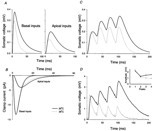
A, the change in somatic membrane potential at the two temperatures subsequent to transient charge injections (total charge 0.1 pC; τ_rise = 0.2 ms; τ_decay = 2.5 ms) at points A and B in cell 1 shown in Fig. 6 (apical tuft and basal dendrite, respectively). There are small reductions in the time to peak and the amplitude but the dominant effect is to extend the whole time course of the potential change. This dramatically affects temporal summation (C), simulated here as the summed response to a short 33 Hz train of synaptic charge injections at point A (to emphasise the effect on summation, a 50 % larger synaptic event was used for the higher temperature to give an equivalent size first response). D, recordings from a layer 2/3 pyramidal cell in response to extracellular stimulation of layer 4. The traces are averages from 20 consecutive trials, again with a larger stimulation at the higher temperature to produce approximately the same size first response. The dominant effect is through the reduction in τ₀: 13.0 ms at 36 °C compared to 40.1 ms at 26 °C. The inset, plotting the amplitude of each successive peak as measured from trough to peak, shows only a minimal temperature difference relative to the overall effect at the fourth peak. B, simulated voltage clamp recordings of synaptic inputs from the same sites as in A. There is only a small change with temperature, reflecting the fact that these clamp currents, like the rise times for EPSPs, are set by C_m and R_i, and are relatively independent of R_m. Of the three cells, this one shows the smallest change in R_iC_m; the change is more obvious in models of the two other cells.

In contrast, cooling only slightly altered the simulated voltage clamp recordings (Fig. 4B). The time to peak is slowed and the peak current reduced, but since the time course is slowed throughout, the integral (i.e. total charge) is barely changed (see below). The effects are more apparent with models of the other two cells. This result highlights the principal determinants of the somatically recorded excitatory postsynaptic current (EPSC) shape, namely the time taken for charge to equilibrate throughout the cell, which is set primarily by C_m and R_i.

DISCUSSION

The findings of most general interest are the estimates of basic electrical parameters for the dendritic trees of layer 2/3 pyramidal cells at physiological temperatures: C_m = 0.78–0.96 μF cm⁻²; R_i = 140–170 Ωcm; G_tot = 7.2- 18.4 nS. This study is the first detailed presentation of experimentally derived, passive cable models for these cells, although a previous study (Larkman et al. 1992) explored the presumptive electrical geometry based on cell morphologies.

We also demonstrate that these measures are temperature dependent. Whilst the capacitance is affected little by cooling to room temperature, the predominant change is an increase in resistivities (membrane and axial) causing the electrotonic structure to become markedly more compact, and the decay of transient responses back to baseline E_m more protracted. The limits for two parameters (R_m and G_sh) are quite broad, but others are tight (C_m, R_i and G_tot) and the temperature effects are likely to be genuine since they are apparent from simple physiological measures (R_N, τ₀ and Q/a₀), which show consistent changes on cooling even though there is considerable variation between cells at any one temperature.

Membrane capacitance and axial resistivity

Our estimate of C_m lies close to the generally accepted value of 1 μF cm⁻², similar to estimates for hippocampal CA3 pyramidal cells (∼0.75 μF cm⁻²; Major et al. 1994), CA3 interneurones (Chitwood et al. 1999) and cerebellar Purkinje cells (Roth & Häusser, 2001), but less than for layer 5 pyramidal cells (∼1.5 μF cm⁻²; Stuart & Spruston, 1998) and motoneurones (∼2.4 μF cm⁻²; Thurbon et al. 1998). It is also exactly as found using nucleated patches, for which the cell membrane area is easily measured (Gentet et al. 2000).

In contrast, our estimate for R_i was higher than for layer 5 pyramidal cells, Purkinje cells and motoneurones, all of which are close to the resistivity of Ringer solution (∼70 Ωcm), but lower than that reported by Major et al. (1994) in CA3 pyramidal cells (170–340 Ω cm at ∼22 °C), although most of this latter discrepancy could be accounted for by the temperature difference. The presence of intracellular organelles might be relevant here. Mitochondria, endoplasmic reticulum and microtubules, amongst others, will serve to reduce the effective conducting medium, and so increase the apparent resistivity. If there is a limit to how small these organelles can be, this effect would be greater for cells with generally thinner dendrites (for instance layer 2/3 and CA3 pyramidal cells and interneurones).

Membrane conductance

The problem of non-unique solutions comes to the fore when considering R_m and G_sh, and consequently limit what we can usefully conclude. However, it seems clear that the change in cell physiology with temperature is predominantly due to changes in membrane conductance.

The results also indicate that the membrane conductance is unevenly distributed in line with several recent studies showing changes in various conductances with distance from the soma in other cell types (Hoffman et al. 1997; Magee, 1998; Johnston et al. 2000; Bekkers, 2001; Korngreen & Sakmann, 2001). Thus, zero shunt models (i.e. uniform R_m) gave extremely bad fits for two cells, and an acceptable one for the third (cell 1), although this was still worse than the optimal fit. A concern previously, when these studies were done using sharp electrodes, was that the requirement for a shunt conductance was due to electrode damage of the somatic membrane. However, for reasons already listed in Methods, and from the fact that two recent studies of other neurone classes have yielded single R_m models from data acquired using patch clamp (Thurbon et al. 1998; Roth & Häusser, 2001), we feel that our findings reflect pyramidal cell biology rather than an artefact of the recording. Of course other distributions of conductances are possible, but at present we can say no more than that the simplest distribution, with uniform R_m, is unlikely in these cells, in contrast to spinal motoneurones and cerebellar Purkinje cells.

The precise distribution of membrane conductances affects the steady-state transfer function of the relevant dendrite (London et al. 1999), dependent as it is on the relationship between R_i and R_m, but this would only be apparent when using two spaced electrodes (e.g. Stuart & Spruston, 1998). It is important to note, though, that for rapid transients, the transfer function is set mainly by C_m and R_i, and so concerns about the wide range of R_m and whether or not it varies are only relevant to synaptic potential decays. Even so, it is clear that dual recordings would improve the modelling and could constrain the models in other ways. Major (Major et al. 1993b; Major, 2001) noted that reciprocity of transfer function at the two recording sites (i.e. the transfer function is identical when recorded in either direction) is a good test for linear behaviour, and Roth & Häusser (2001) demonstrated this in Purkinje cells having first blocked I_h. A second recording site could also further constrain C_m as demonstrated in Fig. 5. Thus, models that are indistinguishable when considering discharge from a somatic injection of charge become increasingly distinct when the injection site is at more distant locations on the dendritic tree. However, whilst suggesting that dual recordings are desirable, there are practical limitations. The behaviour of the models only becomes dramatically different when dealing with inputs into the smallest, high impedance, dendritic branches. Effectively, this would mean recording from dendrites with diameters of less than 0.5 μm, well beyond current technology. Transfer functions could be examined by recording from the apical trunk, but this has only been achieved in much larger cell types (layer 5 pyramids, Stuart & Spruston, 1998; Purkinje cells, Roth & Häusser, 2001), and would still leave uncertainty concerning the basal dendrites. Another possible approach, using voltage-sensitive dyes to examine the spread of depolarisation (Meyer et al. 1997; Antic et al. 1999), would also need to be improved by an order of magnitude to be truly applicable.

Figure 5. Different models can be distinguished by recording from more than one place on the dendritic tree.

The top graph shows the somatic recording of a response to a 1 nA, 0.5 ms somatic current pulse (from cell 1, 26 °C), and two different models at the limits of the acceptable range of values for C_m. The middle graph shows the somatic response to a simulated synaptic input on the apical trunk whilst the bottom graph shows the same for an apical tuft synaptic input (point A in Fig. 6). Thus, if one could determine precisely the nature of the charge injection distally, one could easily distinguish between models that are imperceptibly different in their responses to a somatic charge injection.

In spite of the non-unique solutions for R_m and G_sh, G_tot is remarkably well constrained. The optimal values and acceptable ranges for G_tot are likely to be robust despite being derived from relatively simple models, because the decay after about 15 ms is straightforward, being described well by a single exponential. As such, there is unlikely to be much late redistribution of charge (necessary for very uneven membrane conductances), and with R_i and C_m both being well constrained, we can be reasonably confident in G_tot. Thus, there is probably a limit to how extreme the distribution of conductances can be, and so any other, more complicated distributions of membrane conductances are unlikely to change G_tot appreciably. This also allows us to be confident about the nature of the temperature effect described, since the range of acceptable values for G_tot are completely separate at body and room temperature.

Electrotonic structure of layer 2/3 pyramidal cells

Previous studies have made a distinction between the core electrotonic structure and the raw electrical parameters (Major et al. 1994; Roth & Häusser, 2001). The core structure is the branching pattern of cylinders, each with a unique capacitance, axial resistance and leak conductance. This could be affected if there were problems with the electrophysiological recordings (e.g. inadequate pipette capacitance compensation) or if the reconstructed anatomy did not accurately reflect the true anatomy (e.g. amputation of major dendritic branches, although even this could be minimal as evidenced from the difference between models with and without axons). In practice though, technical problems arise from microscopy limitations (Roth & Häusser, 2001), the most important of which are in accurately measuring the diameter of small dendrites and the contribution of dendritic spines (sampling spine densities, spine areas, collapsing spines onto the dendritic trunk). For instance, the average spine area we used here was derived from a study in adult rats (Peters & Kaiserman-Abramof, 1970). It is known that, although the structure of individual classes appears relatively constant, the proportions of different spine classes do change during development, and so, by using figures derived from adults we may have wrongly estimated the contribution of spines to the total membrane area in our P21 animals. These ‘microscopic’ issues can markedly affect the raw electrical parameters (Major et al. 1994; Major, 2001; Roth & Häusser, 2001). We limit ourselves to two examples here. Increasing the diameters of all dendritic segments by 20 % enlarges the total surface area by just under 12 %, and the net effect of this is to reduce the optimal C_m by 9.5 %, increase the R_i by 45 %, but, because changes in R_m are balanced by those in G_sh, G_tot remains the same. Increasing the average surface area of dendritic spines by 20 %, reduces the capacitance by 7.2 %, whilst R_i and G_tot both remain unchanged. In contrast, the core electrotonic model, which is central to conclusions such as the requirement for uneven distribution of membrane conductances, the nature of the temperature changes, and the filtering effect on inputs at particular synaptic locations, is relatively immune to these modelling problems (Roth & Häusser, 2001).

Our statistical testing of models, whilst ostensibly setting parameter limits, is in fact more relevant to the core model. The test looks at the outputs of models and assesses how far they can differ from the experimental recording. Thus, if it is the case that the membrane area has been wrongly estimated, leading to different values for the individual parameters, all the models will be affected similarly. The cut off point, though, for what is, or is not, an acceptable model, remains unchanged. Consequently, the ranges for individual parameters would be shifted in parallel with the optima but would not be extended (analogous to changing the mean but keeping the same standard deviation).

We also wanted to check whether the models were freely interchangeable. Given that the only ostensible difference between the models was in the membrane conductances; the values for C_m and R_i were very consistent between cells, and previous studies of pyramidal cell morphology failed to distinguish different classes (Larkman, 1991a–c; Larkman et al. 1992), although a progressive increase in cell size with depth below the pia was noted - we wondered whether we could cross fit our reconstructed models with the electrophysiological recordings from other cells. Using cell 1 reconstruction, we derived optimal fits against the responses at room temperature for all the other cells. Of these, only three gave fits that were as good as the cell 1′s own response, and in many cells the fitting program clearly struggled to find the optimum fit. Interestingly though, the optimal values for C_m fell into a relatively narrow range (0.51–1.26) with a unimodal distribution (mean = 0.77; s.d. = 0.18), and correlated well with the distance of the soma from the pia (r = 0.67; n = 22; P < 0.001). The clear implication is that when the electrophysiological data derives from a cell of a different size, the optimal C_m is changed accordingly; the larger the cell providing the physiology, the larger the optimal C_m required to fit the model to the physiology. Put another way, there is a clue to the size of the cell from its physiological response.

The overall electrotonic structure is surprisingly compact. Even the most distal inputs are within a single space constant of the soma, and the great majority of synapses, lying on the basal and apical oblique dendrites, are much closer still. This is made explicit in the iso-efficacy plots in Fig. 6, which show the voltage integral relative to that for an identical somatic input for the three modelled cells which represent the full range of values of input resistance for all 26 cells.

Assessing the models

In recognising the problem of non-uniqueness, one needs to address the issue of how to assess the various models. This, though, is rarely done. Here, we have set limits on the values for the various parameters using the baseline noise to set how much the models can deviate from the data transients. As such, the basic premises are the same as in Major et al.1994; also Thurbon et al. 1998, but we feel that this new approach is an improvement for several reasons: (1) it is intuitively simple and far easier to carry out, (2) it does not necessitate data selection, filtering or averaging, as each raw data trace is compared with the model, (3) the test is sensitive to, but not dominated by, brief ‘escapes’ from the model. Instead, it reflects the performance of the model as a whole - the deviations are mainly low frequency, explaining why the distribution of variances resembles a χ² distribution with a small number of degrees of freedom and (4) the test lends itself to other modelling uses. Indeed, with careful consideration of fitting intervals, it should be possible to combine different experimental tests of a model, such as transfer responses between two electrodes with dissipation of charge injected from a single electrode.

The need for alternative tests of the models is apparent from the range of parameter values (Table 3), particularly R_m and R_i. Merely recording more traces would have helped, and common sense argues against the lower estimates of R_i since they are well below the resistivity of Ringer solution (resistivities at 35 °C; 150 mmNaCl, 54.1 Ωcm; 140 mm KCl, 48.0 Ωcm; 140 mm potassium gluconate ∼65 Ωcm (estimated from potassium acetate conductivity); all values derived from Tables of Conductivity in Lobo, 1989). The real issue, though, is that when modelling current pulses whilst incorporating a shunt conductance, the resistivities are badly constrained. However, as Fig. 5 shows, information about transfer functions (e.g. Stuart & Spruston, 1998; Ulrich & Stricker, 2000) constrains the models considerably.

Effect of cooling

Two previous studies have looked at the effect of cooling using slices from rat visual cortex concluding that synaptic transmission was both less reliable and more variable (Hardingham & Larkman, 1998), that the cells were depolarised, had a higher R_N, but since the threshold for action potentials remained constant, they were more excitable (Volgushev et al. 2000). Here we confirmed the effect on E_m and R_N (see also Thompson et al. 1985), showed that the decay of voltage transients back to baseline E_m is significantly delayed, and through modelling demonstrated that this is primarily due to an increase in membrane conductance. The net effect on synaptic integration is unclear. On the one hand, temporal summation and excitability are greater, but there is a reduction in synaptic reliability - defined here as the probability of transmitter release to a presynaptic action potential. These are clearly issues for the study of synaptic facilitation, potentiation and depression. They will also affect the dynamics of the whole network by subtle effects on the input-output function of individual neurones. At physiological temperatures, a classical view is that the output of a given neurone derives from summation of many synaptic inputs, which individually are fairly reliable. Thus, how predictably a given presynaptic element drives a postsynaptic element depends on the activity in the rest of the network. In contrast, when cooled, a given cell will be more depolarised, and have a higher input resistance. Consequently, individual synaptic inputs will be larger and more likely to elicit an action potential, but this is offset by a reduction in synaptic reliability. Hence, presynaptic activity will still result in postsynaptic firing only some of the time, but this will now be a function more of the unpredictable synaptic contact rather than the network activity. As such, the whole network might behave very differently, with transfer of information more stochastic and less influenced by other network activity, and possibly even changing the receptive field properties of individual cells (cf. Ferster et al. 1996).

REFERENCES

- Antic S, Major G, Zecevic D. Fast optical recordings of membrane potential changes from dendrites of pyramidal neurons. Journal of Neurophysiology. 1999;82:1615–1621. doi: 10.1152/jn.1999.82.3.1615. [DOI] [PubMed] [Google Scholar]
- Barrett EF, Barrett JN, Botz D, Chang DB, Mahaffey D. Temperature-sensitive aspects of evoked and spontaneous transmitter release at the frog neuromuscular junction. Journal of Physiology. 1978;279:253–273. doi: 10.1113/jphysiol.1978.sp012343. [DOI] [PMC free article] [PubMed] [Google Scholar]
- Barrett JN, Crill WE. Specific membrane properties of cat motoneurones. Journal of Physiology. 1974;239:301–324. doi: 10.1113/jphysiol.1974.sp010570. [DOI] [PMC free article] [PubMed] [Google Scholar]
- Bekkers JM. Distribution and activation of voltage-gated potassium channels in cell-attached and outside-out patches from large layer 5 cortical pyramidal neurons of the rat. Journal of Physiology. 2001;525:611–620. doi: 10.1111/j.1469-7793.2000.t01-2-00611.x. [DOI] [PMC free article] [PubMed] [Google Scholar]
- Bekkers JM, Stevens CF. Cable properties of cultured hippocampal neurons determined from sucrose-evoked miniature EPSCs. Journal of Neurophysiology. 1996;75:1250–1255. doi: 10.1152/jn.1996.75.3.1250. [DOI] [PubMed] [Google Scholar]
- Berger T, Larkum ME, Lüscher HR. High Ih channel density in the distal apical dendrite of layer V pyramidal cells increases bidirectional attenuation of EPSPs. Journal of Neurophysiology. 2001;85:855–868. doi: 10.1152/jn.2001.85.2.855. [DOI] [PubMed] [Google Scholar]
- Cauller LJ, Connors BW. Functions of very distal dendrites: experimental and computational studies of layer 1 synapses on neocortical pyramidal cells. In: McKenna T, Davis J, Zornetzer SF, editors. Single Neuron Computation. San Diego: Academic Press; 1992. pp. 199–230. [Google Scholar]
- Chitwood RA, Hubbard A, Jaffe DB. Passive electrotonic properties of rat hippocampal CA3 interneurones. Journal of Physiology. 1999;515:743–756. doi: 10.1111/j.1469-7793.1999.743ab.x. [DOI] [PMC free article] [PubMed] [Google Scholar]
- Clements JD, Redman SJ. Cable properties of cat spinal motoneurons measured by combining voltage clamp, current clamp and intracellular staining. Journal of Physiology. 1989;409:63–87. doi: 10.1113/jphysiol.1989.sp017485. [DOI] [PMC free article] [PubMed] [Google Scholar]
- Durand D, Carlen PL, Gurevich N, Ho A, Kunov H. Electrotonic parameters of rat dentate granule cells measured using short current pulses and HRP staining. Journal of Neurophysiology. 1983;50:1080–1097. doi: 10.1152/jn.1983.50.5.1080. [DOI] [PubMed] [Google Scholar]
- Ferster D, Chung S, Wheat H. Orientation selectivity of thalamic input to simple cells of cat visual cortex. Nature. 1996;380:569–572. doi: 10.1038/380249a0. [DOI] [PubMed] [Google Scholar]
- Fromherz P, Muller CO. Cable properties of a straight neurite of a leech neuron probed by a voltage-sensitive dye. Proceedings of the National Academy of Sciences of the USA. 1994;91:4604–4608. doi: 10.1073/pnas.91.10.4604. [DOI] [PMC free article] [PubMed] [Google Scholar]
- Gentet LJ, Stuart GJ, Clements JD. Direct measurement of specific membrane capacitance in neurons. Biophysical Journal. 2000;79:314–320. doi: 10.1016/S0006-3495(00)76293-X. [DOI] [PMC free article] [PubMed] [Google Scholar]
- Hardingham NR, Larkman AU. Rapid report: the reliability of excitatory synaptic transmission in slices of rat visual cortex in vitro is temperature dependent. Journal of Physiology. 1998;507:249–256. doi: 10.1111/j.1469-7793.1998.249bu.x. [DOI] [PMC free article] [PubMed] [Google Scholar]
- Hodgkin AL, Katz B. The effect of temperature on the electrical activity of the giant axon of the squid. Journal of Physiology. 1965;109:240–249. doi: 10.1113/jphysiol.1949.sp004388. [DOI] [PMC free article] [PubMed] [Google Scholar]
- Hoffman DA, Magee JC, Colbert CM, Johnston D. K+ channel regulation of signal propagation in dendrites of hippocampal pyramidal neurons. Nature. 1997;387:869–875. doi: 10.1038/43119. [DOI] [PubMed] [Google Scholar]
- Holmes WR, Rall W. Extimating the electrotonic structure of neurons with compartmental models. Journal of Neurophysiology. 1992;68:1438–1452. doi: 10.1152/jn.1992.68.4.1438. [DOI] [PubMed] [Google Scholar]
- Jack JJB, Noble D, Tsien RW. Electric Current Flow in Excitable Cells. Oxford: Clarendon Press; 1975. [Google Scholar]
- Johnston D, Hoffman DA, Magee JC, Poolos NP, Watanabe S, Colbert CM, Migliore M. Dendritic potassium channels in hippocampal pyramidal neurons. Journal of Physiology. 2000;525:75–81. doi: 10.1111/j.1469-7793.2000.00075.x. [DOI] [PMC free article] [PubMed] [Google Scholar]
- Katz B, Miledi R. The effect of temperature on synaptic delay at the neuromuscular junction. Journal of Physiology. 1965;181:656–670. doi: 10.1113/jphysiol.1965.sp007790. [DOI] [PMC free article] [PubMed] [Google Scholar]
- Korngreen A, Sakmann B. Voltage-gated K+ channels in layer 5 neocortical pyramidal neurones from young rats: subtypes and gradients. Journal of Physiology. 2001;525:611–620. doi: 10.1111/j.1469-7793.2000.00621.x. [DOI] [PMC free article] [PubMed] [Google Scholar]
- Larkman AU. Dendritic morphology of pyramidal neurones of the visual cortex of the rat: III. Spine distributions. Journal of Comparative Neurology. 1991a;306:332–343. doi: 10.1002/cne.903060209. [DOI] [PubMed] [Google Scholar]
- Larkman AU. Dendritic morphology of pyramidal neurones of the visual cortex of the rat: II. Parameter correlations. Journal of Comparative Neurology. 1991b;306:320–331. doi: 10.1002/cne.903060208. [DOI] [PubMed] [Google Scholar]
- Larkman AU. Dendritic morphology of pyramidal neurones of the visual cortex of the rat: I. Branching patterns. Journal of Comparative Neurology. 1991c;306:307–319. doi: 10.1002/cne.903060207. [DOI] [PubMed] [Google Scholar]
- Larkman AU, Major G, Stratford KJ, Jack JJB. Dendritic morphology of pyramidal neurones of the visual cortex of the rat. IV: Electrical geometry. Journal of Comparative Neurology. 1992;306:137–152. doi: 10.1002/cne.903230202. [DOI] [PubMed] [Google Scholar]
- Larkman AU, Mason A. Correlations between morphology and electrophysiology of pyramidal neurons in slices of rat visual cortex. 1. Establishment of cell classes. Journal of Neuroscience. 1990;10:1407–1414. doi: 10.1523/JNEUROSCI.10-05-01407.1990. [DOI] [PMC free article] [PubMed] [Google Scholar]
- Lobo VMM. Handbook of Electrolye Solutions (Parts A & B) Amsterdam, Oxford, New York, Tokyo: Elsevier Press; 1989. [Google Scholar]
- London M, Meunier C, Segev I. Signal transfer in passive dendrites with nonuniform membrane conductances. Journal of Neuroscience. 1999;19:8219–8233. doi: 10.1523/JNEUROSCI.19-19-08219.1999. [DOI] [PMC free article] [PubMed] [Google Scholar]
- Magee JC. Dendritic hyperpolarization-activated currents modify the integrative properties of hippocampal CA1 pyramidal neurons. Journal of Neuroscience. 1998;18:7613–7624. doi: 10.1523/JNEUROSCI.18-19-07613.1998. [DOI] [PMC free article] [PubMed] [Google Scholar]
- Major G. Passive cable modelling - a practical introduction. In: De Schutter E, editor. Computational Neuroscience: Realistic Modelling for Experimentalists. Washington: CRC Press LLC; 2001. pp. 209–232. [Google Scholar]
- Major G, Evans JD, Jack JJB. Solutions for transients in arbitrarily branching cables: I. Voltage recording with a somatic shunt. Biophysical Journal. 1993a;65:423–449. doi: 10.1016/S0006-3495(93)81037-3. [DOI] [PMC free article] [PubMed] [Google Scholar]
- Major G, Evans JD, Jack JJB. Solutions for transients in arbitrarily branching cables: II. Voltage clamp theory. Biophysical Journal. 1993b;65:450–468. doi: 10.1016/S0006-3495(93)81038-5. [DOI] [PMC free article] [PubMed] [Google Scholar]
- Major G, Larkman AU, Jonas P, Sakmann B, Jack JJB. Detailed passive cable models of whole-cell recorded CA3 pyramidal neurons in rat hippocampal slices. Journal of Neuroscience. 1994;14:4613–4638. doi: 10.1523/JNEUROSCI.14-08-04613.1994. [DOI] [PMC free article] [PubMed] [Google Scholar]
- Meyer E, Muller CO, Fromherz P. Cable properties of dendrites in hippocampal neurons of the rat mapped by a voltage-sensitive dye. European Journal of Neuroscience. 1997;9:778–785. doi: 10.1111/j.1460-9568.1997.tb01426.x. [DOI] [PubMed] [Google Scholar]
- Nelder JA, Mead R. A geometric technique for optimisation. Computer Journal. 1965;7:208–327. [Google Scholar]
- Peters A, Kaiserman-Abramof IR. The small pyramidal neuron of the rat cerebral cortex. The perikaryon, dendrites and spines. American Journal of Anatomy. 1970;127:321–356. doi: 10.1002/aja.1001270402. [DOI] [PubMed] [Google Scholar]
- Press WH, Flannery BP, Teukolshy SA, Betterling WT. Numerical Recipes in C: The Art of Scientific Computing. Cambridge: Cambridge University Press; 1988. [Google Scholar]
- Rall W. Membrane time constant of motoneurons. Science. 1957;126:454. doi: 10.1126/science.126.3271.454. [DOI] [PubMed] [Google Scholar]
- Rall W. Distinguishing theoretical synaptic potentials computed for different soma-dendritic distributions of synaptic input. Journal of Neurophysiology. 1967;30:1138–1168. doi: 10.1152/jn.1967.30.5.1138. [DOI] [PubMed] [Google Scholar]
- Rall W. Time constants and electrotonic length of membrane cylinders and neurons. Biophysical Journal. 1969;9:1483–1508. doi: 10.1016/S0006-3495(69)86467-2. [DOI] [PMC free article] [PubMed] [Google Scholar]
- Rall W. Core conductor theory and cable properties of neurons. In: Kandel ER, editor. Handbook of Physiology, section 1, The Nervous System, Cellular Biology of Neurons. I. Bethesda, MD, USA: American Physiological Society; 1977. pp. 39–98. part 1. [Google Scholar]
- Rapp M, Segev I, Yarom Y. Physiology, morphology and detailed passive models of guinea-pig cerebellar Purkinje cells. Journal of Physiology. 1994;474:101–118. doi: 10.1113/jphysiol.1994.sp020006. [DOI] [PMC free article] [PubMed] [Google Scholar]
- Rinzel J, Rall W. Transient response in a dendritic neuron model for current injected at one branch. Biophysical Journal. 1974;14:759–790. doi: 10.1016/S0006-3495(74)85948-5. [DOI] [PMC free article] [PubMed] [Google Scholar]
- Roth A, Häusser M. Compartmental models of rat cerebellar Purkinje cells based on simultaneous somatic and dendritic patch-clamp recordings. Journal of Physiology. 2001;535:445–472. doi: 10.1111/j.1469-7793.2001.00445.x. [DOI] [PMC free article] [PubMed] [Google Scholar]
- Shelton DP. Membrane resistivity estimated for the Purkinje neuron by means of a passive computer model. Neuroscience. 1985;14:111–131. doi: 10.1016/0306-4522(85)90168-x. [DOI] [PubMed] [Google Scholar]
- Stratford K, Mason A, Larkman AU, Major G, Jack JJB. The modelling of pyramidal neurones in the visual cortex. In: Durbin R, Miall C, Mitchison G, editors. The Computing Neuron. Wokingham: Addison-Wesley; 1989. pp. 296–321. [Google Scholar]
- Stuart G, Spruston N. Determinants of voltage attenuation in neocortical pyramidal neuron dendrites. Journal of Neuroscience. 1998;18:3501–3510. doi: 10.1523/JNEUROSCI.18-10-03501.1998. [DOI] [PMC free article] [PubMed] [Google Scholar]
- Thompson SM, Masukawa LM, Prince DA. Temperature dependence of intrinsic membrane properties and synaptic potentials in hippocampal CA1 neurons in vitro. Journal of Neuroscience. 1985;5:817–824. doi: 10.1523/JNEUROSCI.05-03-00817.1985. [DOI] [PMC free article] [PubMed] [Google Scholar]
- Thurbon D, Field A, Redman SJ. Electrotonic profiles of interneurons in stratum pyramidale of the CA1 region of rat hippocampus. Journal of Neurophysiology. 1994;71:1948–1958. doi: 10.1152/jn.1994.71.5.1948. [DOI] [PubMed] [Google Scholar]
- Thurbon D, Lüscher HR, Hofstetter T, Redman SJ. Passive electrical properties of ventral horn neurons in rat spinal cord slices. Journal of Neurophysiology. 1998;79:2485–2502. doi: 10.1152/jn.1998.79.5.2485. [DOI] [PubMed] [Google Scholar]
- Ulrich D, Stricker C. Dendrosomatic voltage and charge transfer in rat neocortical pyramidal cells in vitro. Journal of Neurophysiology. 2000;84:1445–1452. doi: 10.1152/jn.2000.84.3.1445. [DOI] [PubMed] [Google Scholar]
- Volgushev M, Vidyasagar TR, Chistiakova M, Yousef T, Eysel UT. Membrane properties and spike generation in rat visual cortical cells during reversible cooling. Journal of Physiology. 2000;522:59–76. doi: 10.1111/j.1469-7793.2000.0059m.x. [DOI] [PMC free article] [PubMed] [Google Scholar]
- Williams SR, Stuart GJ. Site independence of EPSP time course is mediated by dendritic I(h) in neocortical pyramidal neurons. Journal of Neurophysiology. 2000;83:3177–3182. doi: 10.1152/jn.2000.83.5.3177. [DOI] [PubMed] [Google Scholar]