Physiological basis of fractal complexity properties of heart rate variability in man

Abstract

The diagnostic and prognostic power of the fractal complexity measure ‘α’ of detrended fluctuation analysis (DFA) has remained mysterious because there has been no explanation of its meaning, particularly in relation to spectral analysis. First, we present a mathematical analysis of the meaning of α, in weighted power-spectral terms. Second, we test this hypothesis and observe correlations between DFA-based and weighted spectral methods of 0.97 (P < 0.0001) for α₁ and 0.98 (P < 0.0001) for α₂. Third, we predict mathematically that even in conventional (unweighted) spectral analysis there should be approximate counterparts to DFA, namely that α₁ and α₂ behave broadly in proportion to the conventional (unweighted) ratios LF/(HF + LF) and VLF/(LF + VLF), respectively, where HF is high frequency, LF is low frequency and VLF is very low frequency. Fourth, we test this hypothesis by physiologically manipulating spectral ratios in healthy volunteers in two ways. The effect of 0.1 Hz controlled breathing on LF/(HF + LF) correlates markedly with the effect on α₁ (r = 0.73, P = 0.01); the effect on VLF/(LF + VLF) correlates markedly with that on α₂ (r = 0.76, P < 0.01). Likewise, with voluntary periodic breathing the reduction in α₂ correlates strongly with that in VLF/(LF + VLF) (r = 0.88, P < 0.001); effects on α₁ and LF/(HF + LF) again clearly correlate (r = 0.73, P = 0.01). Finally, we examine published literature to identify previously undiscussed evidence of the relationship between α₁ and LF/(HF + LF). We conclude that the α₁ and α₂ indices are simply frequency-weighted versions of the spectral ratios LF/(HF + LF) and VLF/(LF + VLF), respectively, multiplied by two (giving a range of 0-2). We can now understand fractal manifestations of physiological abnormalities: depressed baroreflex sensitivity → low LF/HF → low LF/(HF + LF) → low α₁, while periodic breathing → high VLF/LF → high VLF/(LF + VLF) → high α₂. Prognostic associations of α are no longer mysterious.

In patients with cardiovascular disease, inexpensive non-invasive risk stratification remains a holy grail. The complicated pattern of RR interval dynamics has been explored for information for decades (Pagani et al. 1986; Malliani et al. 1991; La Rovere et al. 1998, 2001). Analysis of conventional frequency-domain properties — spectral power in respiratory (‘high frequency’, HF), blood-pressure-mediated (‘low frequency’, LF) and periodic-breathing (‘very low frequency’, VLF) bands — has been fruitful. Moreover, prognostic associations in spectral analysis can be interpreted in the context of physiological processes in each frequency region.

Detrended fluctuation analysis

In the search for improved methods for decoding hidden prognostic messages, parameters arising from non-linear and chaos theory have been identified, with apparent increased diagnostic and prognostic value, especially α₁ and α₂ from detrended fluctuation analysis (DFA; Ho et al. 1997). DFA of heart rate variability was initially presented as a specialised time-domain technique, in which the series of RR intervals undergoes cumulative summing and then segmentation into short segments. Within each segment, the degree of dispersion of the cumulated time series away from its linear trend is measured (as the sum of squares of residuals after subtracting the linear regression line). The total of the squared residuals for the individual segments is calculated for the overall data set. The entire process is then repeated with a different segment length.

Naturally, as the segments become longer, the degree of dispersion away from the linear regression lines within the segments tends to increase, as can be seen in Fig. 1C and D. The rate at which this total dispersion increases as the segments become longer is measured as a slope (α) on a log-log plot (Fig. 1E) over particular regions of segment length, e.g. 4–16 beats or 16–64 beats. Steeper slopes are said to show higher complexity.

Figure 1.

Comparison of calculation of α by DFA and frequency-weighted spectral analysis

In DFA (left panels) the raw data (A) is integrated and detrended (B) and then repeatedly approximated by piecewise linear regression with straight segments of length n heartbeats. For each n, F is defined as the root-mean-square of the residuals (hatched). Examples are given for n = 166 (C) and n = 60 (D). α is the slope of the log-log plot (E) of F against n. The right panels show calculation of α by frequency-weighted power-spectral analysis. The power spectrum (G) is multiplied by the weighting (H), which favours the frequency of interest and decreases proportionally to frequency-squared in both directions. The product (I) is F², from which α is calculated (J) via a plot of log F against log n.

However, in the absence of a conventional physiological interpretation of the α values, it is difficult to understand their observed relationship to pathology and mortality. The extensive body of knowledge of mechanisms of power-spectral heart rate variability is not illuminating because α is assumed to differ fundamentally from spectral analysis (Ho et al. 1997).

In this manuscript we first present a new interpretation of fractal α, which is expressed in terms of the power spectrum, whose relationship to physiological processes is better understood, and validate this empirically. Second, we argue mathematically that α₁ is intimately related to a frequency-weighted LF/(HF + LF) ratio and α₂ to a frequency-weighted VLF/(LF + VLF) ratio. Third, we develop and test the hypothesis that α values are loosely related to conventional (unweighted) spectral ratios. Fourth, we test the hypothesis that physiological manoeuvres, designed to manipulate these LF/(HF + LF) or VLF/(LF + VLF) ratios, predictably affect the α₁ or α₂ fractal correlation measures. Fifth, we review the difference between conventional spectral analysis and the frequency-weighted spectral analysis that is the basis for fractal α. Finally, we examine the published literature for the expected relationship between fractal α and spectral analysis.

METHODS

Approaches to fractal α

To gain an interpretation of α in terms of the power spectrum, we reviewed the standard DFA method of calculating the fractal α value, and have analytically developed new methods: first, a method using the same basic conceptual steps but substituting a novel ‘frequency-weighted’ spectral analysis instead of DFA; second, a method using fewer steps which allows α to be appreciated directly from the ‘frequency-weighted’ power spectrum; and third, a rule-of-thumb approximation using conventional (non-frequency-weighted) power-spectral ratios.

Method 1: by standard DFA.

Figure 1 (left panel) shows the standard calculation(Ho et al. 1997) of fractal scaling exponents α_{1, DFA} and α_2,DFA by DFA. Briefly, the time-series RR interval seqence is divided into equal, non-overlapping segments of length n. In each segment, the data are first integrated, then detrended by subtraction of the least-squares regression line. The root-mean-square residual value over the whole dataset (F_DFA) is then calculated. This operation is performed for divisions of the data into segment lengths (n) of between 4 and 400 data points and the root-mean-square residual F_DFA recorded for each n. Then α is calculated as the regression slope of the log-log plot of F_DFA against n. We have used the ranges of the original clinical paper in this subject (Ho et al. 1997), i.e. α_1,DFA is calculated over the range n = 4 to n = 16 and α_2,DFA between n = 16 and n = 64 (Peng et al. 1995). Other ranges have also been used in the literature, for example n = 4 to n = 11 and n = 12 to n = 400. Ultimately any range can be used; the selection of the boundaries affects the frequency ranges which contribute to the value of α.

Method 2: by frequency-weighted spectral analysis (by steps mathematically equivalent to DFA).

We have derived the previously unsuspected mathematical relationship between DFA and conventional spectral analysis (Appendix 1 and Fig. 1, right panel). For a data segment whose power spectrum is P(F), F²_DFA is effectively equivalent to the expression in eqn (A1). This allows determination of α (which we denote α_1,spectral and α_2,spectral) as the regression slope of log₁₀F²_spectral(n) against log₁₀n, using the power spectrum without the need for DFA.

Method 3: directly from the frequency-weighted power spectrum.

For reasons explained in Appendix 2, an indicative value for α can be obtained directly from the frequency-weighted power spectrum (Fig. 2), namely α₁ ≈ 2(LF_w/[HF_w + LF_w]) and α₂ ≈ 2(VLF_w/[LF_w + VLF_w]). Thus α can be seen to vary from 0 to 2, and approximates to twice the normalised spectral ratio (weighted towards a central frequency of 1/n). For example, α₁, which is centred logarithmically on n = 8, represents approximately twice the ratio of power in oscillations with cycle length just above eight beats divided by the spectral power in the region of the wavelength of eight beats.

Figure 2.

Finding α directly from a frequency-weighted power spectrum

Left panels show method 3. From raw data (A), the power spectrum (B) is calculated, and multiplied by a ‘frequency-weighting’ function (C) to yield LF_w and HF_w components (D). α can be estimated as the average value of LF_w /(HF_w + LF_w) while the weighting function's centre frequency is moved through the range of 1/4 to 1/16 (for α₁) or 1/16 to 1/64 (for α₂). Right panels show method 4, namely that the ‘ordinary’ power spectral ratio LF/(HF + LF) will behave similarly to α₁, but differs in several details (see Discussion).

Method 4: physiological interpretation of α via conventional spectral ratios.

Most conventional literature and current physiological understanding is couched in terms of HF, LF and VLF bands and their ratios. The frequency-weighted spectral ratios which correspond to α differ in several ways (described in the Discussion). Nevertheless, there are some similarities. To calculate α₁ the boundary frequency separating LF_w from HF_w ranges from 1/16 (≈ 0.06) and 1/4 (= 0.25) cycles per beat. The conventional spectral ratio LF/(HF +LF) has its boundary at 0.15 cycles s⁻¹. Likewise α₂ has its boundary between 1/64 (≈ 0.02) and 1/16 (≈ 0.06) cycles per beat, while conventional VLF/ (LF + VLF) has its at 0.04 cycles s⁻¹. Thus, very roughly, in unweighted spectral terms:

Physiological intervention study

Study population.

To compare the different approaches to assessing α, we recruited twelve healthy volunteers with no significant medical history, no medication and no abnormal findings on clinical examination. All subjects gave informed consent and the study was approved by the local Ethical Committee and performed in accordance with the Declaration of Helsinki. The subjects were studied in standardised conditions, in a quiet room at a comfortable temperature, with no smoking, alcohol or caffeine for the previous 12 h. Each subject had three 10 min recordings of heart rate in a random order while seated: (1) normal resting state; (2) voluntarily breathing at 0.1 Hz (using a computerised metronome; Davies et al. 1999) to enhance LF oscillations with respect to HF; and (3) voluntary periodic breathing, to enhance VLF oscillations. Subjects were guided to breathe at a constant respiratory rate with an oscillatory tidal volume of period 1 min. This guidance was provided by visual feedback from a second computer system monitoring ventilation with a pneumotachograph (Francis et al. 1999).

Heart-rate measurement.

The ECG, acquired from a limb lead with a clear R wave, was sampled at 1000 Hz using an analogue-to-digital converter (National Instruments, Austin, TX, USA) and data acquisition software (Labview, National Instruments). RR intervals were subsequently determined automatically by custom software and artefacts due to ectopy corrected by interpolation.

Spectral analysis of power.

For conventional spectral analysis, standard autoregressive spectral methods (Davies et al. 1999) were used. VLF spectral power was determined in the range 0.003- 0.040 Hz, LF in the range 0.040-0.150 Hz and HF in the range 0.150- 0.400 Hz.

For the frequency-weighted spectral analysis to calculate α, RR intervals were retained at one sample per beat in accordance with standard practice for DFA, and therefore in those power spectra, the unit of frequency is cycles per beat rather than cycles s⁻¹ (Hz).

Validation with 24 h recordings

To establish whether the relationship between DFA-based and weighted-spectral-based methods of calculating α persists over recordings of 24 h rather than being limited to short periods of time, Holter data were analysed. Holter recordings, previously obtained for other purposes, from five subjects without heart disease and ten patients with chronic heart failure, were analysed on a standard 24 h ECG analyser (Del-Mar Avionics, Irvine, CA, USA) to obtain the RR interval series. From these data, α₁ and α₂ were calculated by both the DFA method and the weighted spectral method, and the results from the two methods compared.

Statistical analysis

Numerical data of groups are summarised by the mean ± s.e.m. Correlations were calculated by the Pearson product-moment method and differences between measures were assessed by the Bland-Altman standard deviation of differences (s.d.d.). Differences between group means were assessed using Student's t test. A P value of < 0.05 was predefined as significant.

RESULTS

Subjects and recordings

The subjects were all able to perform controlled breathing at 0.1 Hz and all but one were able to perform the voluntary periodic breathing protocol. Mean age was 34 years (s.d. 9 years) and eight were males. Mean height was 172 cm (s.d. 8 cm) and weight 77 kg (s.d. 9 kg).

Comparison of fractal α scaling exponent calculated by DFA and by frequency-weighted spectral analysis

Fractal α₁ and α₂ can be measured by either DFA or frequency-weighted spectral analysis. We performed both analysis methods in all three data sequences from all twelve subjects, yielding 35 measurements by each method for α₁ (Fig. 3A) and 35 for α₂ (Fig. 3B). The correlation between the DFA and frequency-weighted spectral methods of measuring α₁ was 0.97 (P < 0.0001), with s.d.d. 0.07. For α₂, the correlation between methods was 0.98 (P < 0.0001), with s.d.d. 0.08.

Figure 3.

Correlation between methods 1 (DFA) and 2 (frequency-weighted spectral analysis), for α₁(A) and α₂(B).

Comparison of fractal α with conventional spectral ratios

We examined the rules of thumb proposed in method 4, relating α to simple spectral ratios (eqn (1)). The results (Fig. 4) are correlations of 0.86, 0.93, 0.93 and 0.94 (P < 0.0001 for each); s.d.d. values are not calculated as these unweighted spectral ratios are not, mathematically, measures of α.

Figure 4.

Correlation between fractal α and spectral ratios

Upper panels show correlation between spectral ratio 2(LF/[HF + LF]) and fractal α₁ calculated by DFA (A) or by frequency-weighted spectral analysis (B). Lower panels show correlation between spectral ratio 2(VLF/[LF + VLF]) and fractal α₂ calculated by DFA (C) or by frequency-weighted spectral analysis (D).

Effect on fractal measures of intervention designed to enhance spectral LF power relative to HF

The effect of controlled respiration was to increase 2(LF/[HF + LF]) and α₁, as shown in Fig. 5 and Table 1. Importantly, the effect on α₁ closely corresponded to the effect on 2(LF/[HF + LF]), with r = 0.73 (P = 0.01, Fig. 6A). Simultaneously, 2(VLF/[LF + VLF]) and α₂ were reduced. Again, there was a strong correlation between the effects on 2(VLF/[LF + VLF]) and α₂ (r = 0.88, P < 0.001, Fig. 6B).

Figure 5.

Effect on α values of manoeuvres that change spectral ratios

Left panels show the concordant effect of controlled breathing at 0.1 Hz and voluntary periodic breathing on α₁ values (A and B) and on 2(LF/[HF + LF]) (C). Right panels show similar concordant effect on α₂ (D and E) and 2(VLF/[LF + VLF]) (F). Bars indicate standard errors.

Table 1.

Effect of interventions on conventional spectral powers

	HF power(ms2)	LF power(ms2)	VLF power(ms2)
Normal state	365 ± 87	877 ± 195	758 ± 172
Breathing at 0.1 Hz	402 ± 175	3372 ± 642	591 ± 155
Voluntary periodic breathing	320 ± 56	565 ± 148	848 ± 128

Figure 6.

Effect of controlled breathing to attempt to enhance LF relative to HF

A shows that this increases 2(LF/[HF + LF]) in the majority of subjects, and that fractal α₁ is affected in the same direction; the sizes of the two effects are clearly correlated. B shows that both 2(VLF/[LF + VLF]) and fractal α₂ become reduced in all subjects: again the sizes of the changes are strongly correlated.

Effect on fractal measures of intervention designed to enhance spectral VLF power relative to LF

The effect of voluntary periodic breathing was to increase 2(VLF/[LF + VLF]) and α₂, as shown in Fig. 5 and Table 1. Again, the effect on α₂ closely corresponded to the effect on 2(VLF/[LF + VLF]), with r = 0.73 (P = 0.01, Fig. 7B). Simultaneously 2(LF/[HF + LF]) and α₁ were reduced in most subjects. Yet again, there was a strong correlation between the effects on 2(LF/[HF + LF]) and α₁ (r = 0.76, P < 0.01, Fig. 7A).

Figure 7.

Effect of voluntary periodic breathing to attempt to enhance VLF relative to LF

A shows that this increases 2(LF/[HF + LF]) in the majority of subjects, and that fractal α₁ is affected in the same direction; the sizes of the two effects are clearly correlated. B shows that both 2(VLF/[LF + VLF]) and fractal α₂ become reduced in all subjects; again the sizes of the changes are strongly correlated.

Comparison of α calculated by DFA and by frequency-weighted spectral analysis: validation with 24 h ECG recordings

Twenty-four hour Holter ECG recordings, which had been obtained for clinical purposes, were examined in ten patients with chronic heart failure aged 65 years (s.d. 10 years). We also examined 24 h recordings from five subjects without cardiovascular disease, aged 45 years (s.d. 13 years). The correlation between the DFA and frequency-weighted spectral methods of measuring α₁ was 0.99 (P < 0.0001). For α₂, the correlation between methods was also 0.99 (P < 0.0001). The scatterplots are shown in Fig. 8.

Figure 8.

Agreement between DFA and spectral methods of calculating α

Correlation between methods 1 (DFA) and 2 (frequency-weighted spectral analysis), for α₁ (A) and α₂ (B) using data from 24 h ECG recordings in 10 patients with chronic heart failure (○) and 5 subjects without cardiovascular disease (•).

DISCUSSION

We have provided a framework for understanding the physiological basis of fractal complexity in heart rate variability. First, we showed how the α measure of fractal complexity can be re-expressed mathematically in terms of conventional power-spectral analysis in a manner to allow the physiological meaning to be widely appreciated. Second, we demonstrated the strong agreement between fractal complexity as measured by DFA and by frequency-weighted power-spectral approach. Third, we related the fractal complexity measures indirectly to very simple conventional power-spectral ratios, such as the LF/ (HF + LF) ratio. Fourth, we showed how, with this physiological understanding of fractal complexity measures, interventions can be designed which affect the fractal complexity measures in predictable ways. This allows a rational mechanism for the prognostic capacity of measurements of fractal complexity to be proposed.

Physiological origin of apparent fractal complexity (α)

Understanding α in power-spectral terms.

Our mathematical analysis, outlined in Appendix 2, reveals that the fractal scaling property α, whose calculation has previously been possible only by DFA, can in fact be obtained via conventional Fourier analysis (eqn (A4)). Although this equation may appear complicated, it contains two terms which between them address the total weighted spectral power of the data. The segment length (n) is used to divide this total power into the two parts, using the frequency 1/n as the cutoff. A simplified interpretation using unweighted spectral powers can be derived, namely α₁ ≈ 2(LF/[HF + LF]) and α₂ ≈ 2(LF/[HF + LF]). Figure 3 demonstrates the strength of the equivalence between α and even this very simplified interpretation.

Differences between fractal α and conventional power-spectral ratios.

The α measure of fractal complexity closely resembles conventional power-spectral ratios, but this analysis identifies the differences between them.

The most obvious difference is that α standardises oscillation periods in heartbeats rather than in seconds as in conventional spectral analysis. For example, α₁, in all patients, refers to the ratio of powers of oscillations whose periods are longer or shorter than approximately eight heartbeats (regardless of heart rate in beats per minute). In contrast, conventional LF/(HF + LF) addresses the ratio of powers of oscillations with periods 6–20 and 2.5-6 s; if the heart rate is ≈60 beats min⁻¹, this means periods of 6–20 and 2.5-6 heartbeats, respectively, whereas if the heart rate is ≈120 beats min⁻¹, this means periods of 3–10 and 1.25-3 heartbeats, respectively. A priori, it is not obvious which approach is better. The time-based approach has become conventional in spectral analysis for historical reasons. Any worker accustomed to thinking about time in seconds (i.e. frequency in hertz) might argue that in tachycardia, α is addressing a higher-frequency region of the power spectrum, and that therefore differences in heart rate between subjects may be enough to generate differences in measured α even if there is no alteration in the actual modulation of heart rate. One counterargument might be that, since it is respiration that drives the HF oscillation, and tachypnoea can occur alongside tachycardia, comparisons between patients should be made at fixed numbers of heartbeats.

The second difference is in the range of frequencies considered and their weighting. Conventional power-spectral ratios assess power in fixed (in Hertz) frequency ranges and give equal weighting to all frequencies within these ranges. In contrast, α addresses, in principle, all frequencies simultaneously, but strongly favours frequencies close to the centre of the range of interest, with frequencies on the outskirts (in either direction) de-emphasised. For example, α₁ can be conceptualised as the average of the ratio of the shaded areas in Fig. 2D as the cutoff is moved from 4 to 16. Viewed even more simply, by taking the logarithmic midpoint of this range, α is approximately equal to the ratio of the shaded areas when the cutoff is at 8 heartbeats per cycle. Note that the entire power spectrum of the data is involved, but that frequencies far from the 4–16 range are markedly de-emphasised. Thus, even if the heart rate is 72 beats min⁻¹, so that 1/8 beats equals 0.150 Hz, calculation of α₁ will never precisely coincide with the ratio 2(LF/[HF + LF]).

Experimental verification of physiological interpretation of α

First, despite the differences discussed above, our data show considerable correlation between α (calculated by either DFA or by the frequency-weighted power-spectral approach) and the conventional power-spectral ratios in our observational study (Fig. 4).

Second, our experiments show that when we intervene to manipulate the LF/(HF + LF) or VLF/(LF + VLF) ratios, α₁ and α₂ are found to change in the way expected from our mathematical analysis (Figs 5, 6 and 7). We argue, therefore, that α should not be considered to be a unique cardiovascular indicator in a separate ‘fractal’ class from conventional power-spectral analysis, because it has a clear and comprehensible grounding in spectral analysis and behaves in the predicted manner in response to simple intervention.

The third source of verification is examination of previously published data from other groups.

Examining previously published fractal α data.

First, fractal α has been examined in 114 healthy subjects (Pikkujamsa et al. 1999) across a wide age range (1-82 years). The authors concluded that fractal α is not markedly dependent on age, and therefore must be fundamentally different from spectral heart rate variability, since (for example) HF and LF powers increase from childhood to the age of approximately 20 years and then decline. The realisation from our present work, however, is that α₁ is closely related to 2(LF/[HF + LF]) and α₂ to 2(VLF/[LF + VLF]). Although averaged values of LF/(HF + LF) were not reported, there is a table of mean values of HF, LF and VLF which can be used to calculate estimates. Since there are four age groups and two times of day, eight points are available for correlation. Remarkably, the correlation between fractal α₁ and 2(LF/[HF + LF]) is 0.96 (P < 0.05). Furthermore the correlation between fractal α₂ and 2(VLF/[LF + VLF]) is also 0.96 (P < 0.05).

Second, after the DIAMOND trial of dofetilide in myocardial infarction, a substudy (Huikuri et al. 2000) presented mean values of LF/HF ratio of edited α₁ in four non-overlapping groups of patients (dofetilide versus placebo, survivors versus non-survivors). From the presented data, the correlation between α₁ and 2(LF/[HF + LF]) was 0.95 (P < 0.05).

Third, a study of patients after myocardial infarction and healthy controls (Perkiomaki et al. 2001) which reported data for three time periods (providing 6 measurements) reveals a correlation between α₁ and 2(LF/[HF + LF]) of 0.92 (P < 0.01).

Fourth, the early workers on fractal α in chronic heart failure and healthy controls (Ho et al. 1997) displayed on a two-dimensional grid the probability of diagnosis of heart failure given any combination of α₁ and α₂. They observed normal subjects clustered at the higher part of the α₁ range and at the lower part of the α₂ range. The other three quadrants (lower α₁ or higher α₂ or both) were dominated by patients with chronic heart failure. At that time, no explanation was available for this. We can now offer an explanation in spectral terms. Heart failure is characterised by a decrease in the 2(LF/[HF + LF]) ratio, so that α₁ is lower. Heart failure is also frequently associated with periodic breathing, which can generate corresponding VLF rhythms in heart rate (Mortara et al. 1997). This, alone or in association with the reduced LF, may increase the 2(VLF/[LF + VLF]) ratio and α₂.

Conclusions

The α variable calculated by DFA of heart rate, recently identified to have diagnostic and prognostic value in cardiovascular disease, is considered by previous workers to be a fractal measure, by implication different in nature from conventional spectral analyses.

We have shown, by a novel analysis of the mathematics underlying DFA, that α is fundamentally related to a weighted form of spectral analysis. Clinical data confirm this relationship between α and both weighted and conventional spectral ratios such as LF/(HF + LF). This relationship is seen not only among different subjects but also within one subject when interventions are performed to displace spectral ratios away from the individual subjects’ resting values.

Thus, α cannot any longer be considered to be in a different class of measurements from spectral analysis.

Armed with this information, it becomes clear why, in chronic heart failure, α₁ is low (namely its relationship to LF/(HF + LF)) and α₂ sometimes high (namely its relationship to VLF/(LF + VLF)). It can therefore be speculated that the known adverse prognostic significance of low LF and of periodic breathing (which can generate VLF) might explain the prognostic associations of α. Why α has appeared in the hands of some workers to be more predictive than conventional spectral analysis is not yet clear, but the first step in elucidating this is to state clearly the specific differences between the two types of measure, namely: (i) the frequency ranges are different and, moreover, for DFA fixed in cycles per beat whereas for conventional spectral analysis they are fixed in cycles s⁻¹ (Hz) and the relationship between these depends on heart rate; and (ii) α frequency weights power spectra, favouring the centre frequency, de-emphasising others in proportion to frequency-squared in both directions, while conventional spectral analysis gives equal weight to all frequencies within its band of interest.

GLOSSARY

F

root-mean-square of residuals after integration and detrending

N

length of data set (samples)

P(f)

power spectrum

f

frequency of signal component (cycles per sample)

k₁ and k₂

constants

n

length of regression segment (samples)

α

slope of log₁₀(F) on log₁₀(n)

LF_w

frequency-weighted power within lower frequency region of the spectrum

HF_w

frequency-weighted power within higher frequency region of the spectrum

APPENDIX 1

Calculating fractal α directly from the power spectrum

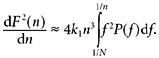
If the RR interval signal of length N samples is expressed as a power series (Zwillinger, 1996), the effect of integration and detrending (Weisstein, 1999) on each term can be determined analytically. For signals of wavelength longer than n, the dominant term is proportional to n⁴ and f². For shorter-wavelength signals, it is proportional to 1/f². At any n, F² of DFA can then be expressed directly from total power ∫¹_1/NP(f) df by appropriate frequency-weighting (Willson et al. 2002).

(A1)

where k₁ ≈ (2π)⁴/1440 and k₂ ≈ 1/2.

α, the slope of log₁₀(F²) against log₁₀(n), can thus be calculated as easily via this route (α_spectral) as via DFA (α_DFA).

APPENDIX 2

Identifying the equivalences between fractal α and LF/(LF + HF) and VLF/(VLF + LF)

Since α is effectively d log₁₀(F)/d log₁₀(n), the chain rule reveals that:

(A2)

To find α we need dF²/dn, which we can obtain from eqn (A1)(Willson et al. 2002) after eliminating the discontinuity artefact:

(A3)

Inserting eqns (A1) and (A3) into eqn (A2), we obtain after several steps: _1/n

(A4)

Although eqn (A4) may appear complicated, it contains two terms which between them address the total spectral power of the data. The segment length (n) is used to divide this total power into the two parts, using the frequency 1/n as the cutoff.

The first term refers to frequencies below 1/n, but weighted in proportion to the square of the frequency and scaled to give a weighting of 1 at the frequency 1/n itself, thus ∫¹_1/Nf²n²P(f)df. The second term refers to frequencies at or above 1/n, weighted in proportion to 1/f², and again scaled to give a weighting of 1 at the frequency of 1/n, yielding the term ∫¹_1/nP(f)/(f²n²)df.

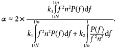
The meaning is that fractal α can be conceptualised as a ratio between two weighted components of the total power spectrum of the data, as illustrated in Fig. 2. We can derive a very simple expression for the ‘fractal correlation coefficient’, α, based on frequency-weighted higher-frequency power HF_w= k₂ ∫¹_1/nP(f)/(f²n²) and frequency-weighted lower-frequency power LF_w = k₁ ∫^1/n_1/NP(f)df:

Strictly, HF_w and LF_w are best obtained from the power spectrum by frequency weighting, as we have done to form α_1,spectral and α_2,spectral (see Fig. 2). However, simple rule-of-thumb estimates can be obtained from unweighted power-spectral ratios:

Alternative, and mathematically identical, expressions are:

REFERENCES

- Davies LC, Francis DP, Jurak P, Kara T, Piepoli M, Coats AJ. Reproducibility of methods for assessing baroreflex sensitivity in normal controls and in patients with chronic heart failure. Clinical Science. 1999;97:515–522. [PubMed] [Google Scholar]
- Francis DP, Davies LC, Piepoli M, Rauchhaus M, Ponikowski P, Coats AJ. Origin of oscillatory kinetics of respiratory gas exchange in chronic heart failure. Circulation. 1999;100:1065–1070. doi: 10.1161/01.cir.100.10.1065. [DOI] [PubMed] [Google Scholar]
- Ho KK, Moody GB, Peng CK, Mietus JE, Larson MG, Levy D, Goldberger AL. Predicting survival in heart failure case and control subjects by use of fully automated methods. Circulation. 1997;96:842–848. doi: 10.1161/01.cir.96.3.842. [DOI] [PubMed] [Google Scholar]
- Huikuri HV, Makikallio TH, Peng CK, Goldberger AL, Hintze U, Moller M. Fractal correlation properties of R-R interval dynamics and mortality in patients with depressed left ventricular function after acute myocardial infarction. Circulation. 2000;101:47–53. doi: 10.1161/01.cir.101.1.47. [DOI] [PubMed] [Google Scholar]
- La Rovere MT, Bigger JT, Jr, Marcus FI, Mortara A, Schwartz PJ. Baroreflex sensitivity and heart-rate variability in prediction of total cardiac mortality after myocardial infarction. Lancet. 1998;351:478–484. doi: 10.1016/s0140-6736(97)11144-8. [DOI] [PubMed] [Google Scholar]
- La Rovere MT, Pinna GD, Hohnloser SH, Marcus FI, Mortara A, Nohara R, Bigger JT, Jr, Camm AJ, Schwartz PJ. Baroreflex sensitivity and heart rate variability in the identification of patients at risk for life-threatening arrhythmias. Circulation. 2001;103:2072–2077. doi: 10.1161/01.cir.103.16.2072. [DOI] [PubMed] [Google Scholar]
- Malliani A, Pagani M, Lombardi F, Cerutti C. Cardiovascular neural regulation explored in the frequency domain. Circulation. 1991;84:484–492. doi: 10.1161/01.cir.84.2.482. [DOI] [PubMed] [Google Scholar]
- Mortara A, Sleight P, Pinna GD. Abnormal awake respiratory patterns are common in chronic heart failure. Circulation. 1997;96:246–252. doi: 10.1161/01.cir.96.1.246. [DOI] [PubMed] [Google Scholar]
- Pagani M, Lombardi F, GuETTIZZ S. Power spectral analysis of heart rate and arterial pressure variabilities. Circulation Research. 1986;59:178–193. doi: 10.1161/01.res.59.2.178. [DOI] [PubMed] [Google Scholar]
- Peng CK, Havlin S, Stanley HE, Goldberger AL. Quantification of scaling exponents and crossover phenomena in nonstationary heartbeat time series. Chaos. 1995;5:82–87. doi: 10.1063/1.166141. [DOI] [PubMed] [Google Scholar]
- Perkiomaki JS, Zareba W, Kalaria VG, Couderc J, Huikuri HV, Moss AJ. Comparability of nonlinear measures of HRV between long- and short-term electrocardiographic recordings. American Journal of Cardiology. 2001;87:905–908. doi: 10.1016/s0002-9149(00)01537-x. [DOI] [PubMed] [Google Scholar]
- Pikkujamsa SM, Makikallio TH, Sourander LB, Raiha IJ, Puukka P, Skytta J, Peng CK, Goldberger AL, Huikuri HV. Cardiac interbeat interval dynamics from childhood to senescence. Circulation. 1999;100:393–399. doi: 10.1161/01.cir.100.4.393. [DOI] [PubMed] [Google Scholar]
- Weisstein EW. Concise Encyclopedia of Mathematics. Boca Raton, FL, USA: CRC Press; 1999. [Google Scholar]
- Willson K, Francis DP, Wensel R, Coats AJS, Parker K. Relationship between detrended fluctuation analysis and spectral analysis of heart rate variability. Physiological Measurement. 2002;23:385–401. doi: 10.1088/0967-3334/23/2/314. [DOI] [PubMed] [Google Scholar]
- Zwillinger D. Standard Mathematical Tables and Formulae. Boca Raton, FL, USA: CRC Press; 1996. [Google Scholar]