Independence of extracellular tortuosity and volume fraction during osmotic challenge in rat neocortex

Abstract

The structural properties of brain extracellular space (ECS) are summarised by the tortuosity (λ) and the volume fraction (α). To determine if these two parameters were independent, we varied the size of the ECS by changing the NaCl content to alter osmolality of bathing media for rat cortical slices. Values of λ and α were extracted from diffusion measurements using the real-time ionophoretic method with tetramethylammonium (TMA⁺). In normal medium (305 mosmol kg⁻¹), the average value of λ was 1.69 and of α was 0.24. Reducing osmolality to 150 mosmol kg⁻¹, increased λ to 1.86 and decreased α to 0.12. Increasing osmolality to 350 mosmol kg⁻¹, reduced λ to about 1.67 where it remained unchanged even when osmolality increased further to 500 mosmol kg⁻¹. In contrast, α increased steadily to 0.42 as osmolality increased. Comparison with previously published experiments employing 3000 M_r dextran to measure λ, showed the same behaviour as for TMA⁺, including the same constant λ in hypertonic media but with a steeper slope in the hypotonic solutions. These data show that λ and α behave differently as the ECS geometry varies. When α decreases, λ increases but when α increases, λ rapidly attains a constant value. A previous model allowing cellular shape to alter during osmotic challenge can account qualitatively for the plateau behaviour of λ.

The structure of the extracellular space (ECS) of the brain can be approximated by two parameters, the volume fraction (α) and the tortuosity (λ) (Nicholson & Phillips, 1981). Volume fraction is the ratio of the volume of ECS to total tissue volume in a representative elementary volume of brain tissue. Tortuosity is defined as λ = √(D/D*) where D (cm² s⁻¹) is the free (aqueous) diffusion coefficient of the molecule and D* (cm² s⁻¹) is the effective (apparent) diffusion coefficient in brain tissue. Tortuosity is related to the hindrance imposed on a diffusing particle by the cellular elements, and possibly the extracellular matrix (Nicholson & Syková, 1998; Nicholson, 2001). A quantitative understanding of the structure of the ECS is important for many issues, including volume transmission (Fuxe & Agnati, 1991; Agnati et al. 2000), the interpretation of diffusion-weighted magnetic resonance imaging (MRI) (Nicolay et al. 2001; Norris, 2001), the treatment of brain ischaemia and other traumas (Syková, 1997) and the delivery of drugs and therapeutic agents (Saltzman, 2001). Here we used osmotic stress to study the relationship between volume fraction and tortuosity.

Both α and λ can be measured by analysing the diffusion of molecules that remain predominantly in the ECS after release from a point source (Nicholson & Phillips, 1981; Nicholson & Syková, 1998; Nicholson, 2001). For a specific brain structure, in the sense that the geometry is preserved, one would anticipate an inverse relationship between α and λ, because a reduction in the volume of the ECS might be expected to increase hindrance to diffusion. This study used osmotic stress, induced by varying the NaCl content of the artificial cerebrospinal fluid (ACSF) to change the size of the ECS. It is known (Križaj et al. 1996), and further confirmed in the present study, that such manipulation causes water to relocate between the ECS and the intracellular compartments of brain tissue.

Tortuosity and volume fraction were measured with the real-time ionophoretic (RTI) method using tetramethylammonium (TMA⁺, 74 M_r), the small extracellular cationic probe (Nicholson & Phillips, 1981; Nicholson, 1993). Measurements of extracellular field potentials and water content provided supporting data. Rat neocortical slices were used because they provided a homogenous, isotropic tissue and good control of the extracellular ionic environment. We emphasise that our goal was not to study the effect of osmotic stress on tissue but to use the challenge to explore a fundamental question about the relationship between structural parameters of brain tissue.

Over the range of osmolalities employed, we found that there was no simple relationship between α and λ. Tao (1999) measured λ under similar osmotic challenge but using 3000 M_r dextran and the integrative optical imaging (IOI) method. Comparing the results from that paper with the data reported here leads to new insights into the structural constraints imposed by the ECS and has led to a novel theoretical model (Chen & Nicholson, 2000). Some results have been published in abstract form (Nicholson et al. 1998).

The study by Križaj et al. (1996) used the whole turtle cerebellum whereas the present study employs slices of a mammalian neocortex and therefore is more relevant to other studies of slice physiology. The turtle study also did not explore hypotonic challenges extensively. The paper by Tao (1999) looked at a similar range of osmotic stresses in the same slice preparation as used here but used a significantly larger molecule and IOI, a technique that permits measurement of the effective diffusion coefficient, and hence tortuosity, but not volume fraction. The present study has used the RTI method with TMA⁺, as frequently used in other studies; importantly, this enables both tortuosity and volume fraction to be measured simultaneously. The theoretical paper by Chen & Nicholson (2000) is based on the data reported in the present paper and therefore complements this study. Because the theory is quite complex and likely to be applicable widely, it was published separately.

METHODS

Rat neocortical slices

All experiments were carried out at NYU School of Medicine in accordance with NIH guidelines and local Institutional Animal Care and Use Committee (IACUC) regulations. Brain slices were obtained from young adult female Sprague-Dawley rats (140-160 g). The animals were anaesthetised with sodium pentobarbital (65 mg kg⁻¹) administered in the intraperitoneal cavity, decapitated and the cerebral cortex removed into chilled ACSF (defined below). Coronal slices were cut at a thickness of 400 μm using a Vibroslice (Camden Instruments, Camden, UK). After incubation in normal ACSF at room temperature for an hour or more, a slice was transferred to a custom-built submersion chamber where the slice was maintained at 34 ± 1 °C under ACSF that flowed at about 1 ml min⁻¹. Diffusion measurements were made in cortical layers III-VI, but no differences were noted in different layers.

Osmotic challenges

The normal isotonic ACSF had the following composition (mm): NaCl 115, KCl 5, NaHCO₃ 35, NaH₂PO₄ 1.25, MgCl₂ 1.3, CaCl₂ 1.5, d-glucose 10 and TMA⁺ chloride 0.5. The TMA⁺ was added to provide a baseline and control value for the diffusion measurements. This formulation resulted in an osmolality of about 305 mosmol kg⁻¹ as determined with a freezing point-depression osmometer (Osmette, Precision Systems, MA, USA) and the errors in the osmolalities were within ± 3 mosmol kg⁻¹. The ACSF solutions were gassed continuously with 95 % O₂-5 % CO₂ to maintain a pH of 7.5.

Three hypotonic ACSF solutions were used with osmolalities of approximately 250, 200, and 150 mosmol kg⁻¹, prepared by reducing the NaCl content of the isotonic solution. Four hypertonic solutions were made by adding NaCl to ACSF to increase the osmolalities to approximately 350, 400, 450 and 500 mosmol kg⁻¹.

After a brain slice had been transferred into the recording chamber and allowed to equilibrate with the warm flowing ACSF, several measurements were made in isotonic ACSF to obtain the control diffusion parameters. Then the isotonic ACSF was quickly replaced (within 1 min) with either a hypo- or hypertonic ACSF, the slice allowed to re-equilibrate for 15 min and a sequence of diffusion measurements made. Finally, the flowing solution was switched back to isotonic ACSF and, after a further interval of 15 min, another sequence of measurements was made to record the recovery behaviour. We found that 15 min was an adequate period to reach a steady state for diffusion measurements, despite the fact that diffusion processes are too slow to allow the changed NaCl concentration to become uniform throughout the slice in such a short period of time (Nicholson & Hounsgaard, 1983). It appears, therefore, that the osmotically driven water movements are more rapid than the diffusion-driven movement of solute.

Field potentials

Field potentials were recorded in eight experiments to monitor synaptic transmission in the neocortex under normal conditions, and during osmotic challenge and recovery. The recordings were made in an interface chamber (Medical Systems model BSC-BU with Hass top, now distributed by Harvard Apparatus Inc., Holliston, MA, USA) perfused with ACSF at 1.7 ml min⁻¹ and maintained at 34 °C with identical composition to that used in the diffusion measurements. Stimuli (duration 20–30 μs) were delivered every 15 s through a bipolar twisted wire electrode placed at the border of white matter and layer VI. Field potentials were recorded in cortical layer III using glass micropipettes filled with 2 m NaCl (resistance 10–20 MΩ). The responses were digitised and stored on a PC. An average of four consecutive responses was used for illustration.

Following the equilibration of the slice in the recording chamber in isotonic ACSF, the field potentials were recorded for at least 15 min to ensure the stability of the response. Isotonic ACSF was exchanged for either hypotonic or hypertonic ACSF and the slices were allowed to equilibrate for 15 min. Field potentials were recorded under the new solution for 15 min then the slices were perfused again with isotonic ACSF and the responses recorded during recovery. In some experiments, the slices were successively perfused with ACSF solutions of increasing hypotonicity or hypertonicity followed by a single recovery period in isotonic ACSF.

Water content

Water content of brain slices was measured using the wet-weight/dry-weight method, after incubation in isotonic ACSF and during osmotic challenge (Križaj et al. 1996). To quantify water content, each slice was removed from the incubation chamber on a plastic spatula and excess ACSF carefully removed. The wetweight of the slice was determined on a pre-weighed piece of aluminium foil. Then the slice and foil were baked in a precision oven at 85°C overnight and next day the dry-weight was measured. The water content of the slice was determined as a difference between wet-weight and dry-weight and expressed as a percentage of wet-weight.

The experimental sequence was as follows. One hour after dissection and incubation at room temperature, the slices were placed in isotonic ACSF maintained at 34 °C. Following 15 min of equilibration, a group of slices was weighted (control group). The remaining slices were transferred to the hypotonic or hypertonic ACSF and the wet-weight was measured after 30 min of incubation (osmotically challenged groups). During all incubations, slices were submerged in ACSF (gassed with 95 % O₂-5 % CO₂) at 34 °C to ensure identical conditions with those for diffusion measurements. For each time point, a group of 3–4 slices was used and the values were averaged; n represents the number of groups.

TMA⁺ diffusion measurements

Diffusion measurements using TMA⁺ were made using the RTI method and ion-selective microelectrodes (ISMs), as described previously (Nicholson & Phillips, 1981; Nicholson, 1993). In summary, TMA⁺ was released by ionophoresis from a micropipette and the local concentration measured with an ISM located about 100 μm from the release site. To maintain accurate spacing, the bent ionophoresis microelectrode and ISM were glued together in a fixed array, using rapidly curing methacrylate polymer (Durabase, Reliance, Worth, IL, USA) and the spacing of the tips measured before and after each experiment using a compound microscope equipped with a graticule.

In order to extract the diffusion parameters, it is necessary to use equations describing the diffusion process. These have been derived and elaborated elsewhere (Nicholson & Phillips, 1981; Nicholson, 2001) and are summarised here. The concentration C (mm) at time t (s) and distance r (cm) from a point source that releases ions during a period t_p (s) is given by:

(1a)

where u is a dummy variable and G(u) is defined by:

(1b)

and p±(r,u) and q ± (r) are defined by:

(1c)

In equation 1a, H is the Heaviside step function and erfc is the complementary error function. The source amplitude, Q = In_t/F (mol l⁻¹), is the ionophoresis source term, where I (amps) is the current, typically 100 nA, n_t is the transport number for TMA⁺ and a specific ionophoresis electrode, and F (9.6485 × 10⁻⁴ C mol⁻¹) is the Faraday constant. The term k’ (s⁻¹) represents linear clearance (i.e. removal proportional to extracellular TMA⁺ concentration, [TMA⁺]). Many diverse clearance processes in the ECS reduce to linear terms for small values of the variables (e.g. Fenstermacher et al. 1974; Bungay et al. 1990; Saltzman & Radomsky, 1991) and this has been found appropriate in numerous studies of TMA⁺ diffusion (reviewed in Nicholson, 2001). Note that eqn (1) can be generalised for anisotropic diffusion (see equation (52) in Nicholson, 2001) but that is not required for the rat neocortex (Voříšek & Syková, 1997a).

If the ionophoretic pulse is applied for a very long time, then eqn (1b) becomes:

(2)

This is relevant because a continual positive bias current of 20 nA was applied to the ionophoresis microelectrode (which contained 150 mm TMA⁺ chloride) to maintain a constant n_t and eqn (2) describes the baseline TMA⁺ concentration under these conditions. The concentration defined in eqn (1) can be normalised by dividing by eqn (2) so that:

(3)

Using the simplex non-linear curve fitting algorithm (Press et al. 1986), eqn (1) was fitted to experimental data and α, D* and k’ extracted using the programs VOLTORO and WALTER (both available for the PC from C. Nicholson). The value of λ was calculated from D* when D was known; then the value of α could be obtained provided that n_t was known.

Both n_t and D were obtained by making diffusion measurements in 0.3 % agarose (NuSieve, FMC BioProducts, Rockland, ME, USA) dissolved in 154 mm NaCl solution containing 0.5 mm TMA⁺ chloride. By definition, in a free medium such as agarose, α = 1, λ = 1 and k’ = 0. The TMA⁺ was added here, and in the ACSF, to provide a stable reference baseline for the concentration measurements. All measurements in agarose were made at 34 ± 1 °C. In practice, only the n_t value obtained from agarose measurements was needed from these experiments because D_TMA (cm² s⁻¹) was already accurately known, as a function of temperature T (degrees kelvin), (Nicholson, 2001)

(4)

Knowledge of this value was used to confirm the accuracy of the optically measured electrode spacing.

Calculation of the water contents of the extracellular and intracellular compartments

The full analysis is provided in Križaj et al. 1996 and only the relevant formulae are reproduced here. We assumed that brain tissue comprised three compartments, extracellular water (designated by subscript ‘e’), intracellular water (subscript ‘i’) and the dry solids (subscript ‘d’). The total amount is designated by subscript ‘t’. Then, denoting mass by m, the total mass m_t of a given sample is:

(5)

The two quantities most often used to describe the degree of hydration of tissue are the water content per wet-weight, ω, and the water content per dry-weight, ε, defined by:

(6)

and so ω and ε are related by:

(7)

By measuring extracellular volume fraction, α, using ionophoresis of TMA⁺, the mass-ratios m_i/m_d and m_e/m_d can be determined independently. In order to do this one has to assume (Križaj et al. 1996) that the densities of the three compartments are close to unity, then:

(8)

(9)

and

(10)

The behaviour of ε = (m_i+m_e)/m_d indicates whether the tissue swells or shrinks while m_i/m_d and m_e/m_d indicate how water partitions between compartments.

A further question can be answered from this analysis, namely how the linear dimension of the slice changes as the slice is subject to osmotic stress. If m_t denotes the total mass of the slice in normal solution and m_t’ is the mass under osmotic stress, then denoting a linear dimension by x, and assuming that swelling or shrinking occurs in a similar way in each dimension, it follows that:

(11)

Statistical treatment of diffusion measurements

Data from 31 rats were used with between 3–6 slices from each rat. A number of additional data sets were discarded because the ISM calibration and response time were not maintained throughout the experiment. In the data presented, only one osmotic challenge and recovery was performed per slice and the value of n cited in statistics represents the number of slices. We assumed that different slices from the same rat represented independent samples. Curve fitting procedures used at least 20 uniformly spaced data points and as many as 250; these numbers of data points effectively removed the influence of noise from the fitting procedure.

RESULTS

The goal of the experiments was to explore the relation between λ and α using osmotic stress to change these two parameters. We also did supporting experiments to measure field potentials and water content to ensure that artefacts did not corrupt our interpretations.

Field potentials

We used eight rats to establish that the slices we used could sustain synaptic activity before and after the osmotic challenges and to document the changes in activity during the osmotic stress. We recorded extracellular field potentials, as detailed in the Methods section.

Similar results were obtained in all experiments. Figure 1A shows results from one experiment where a slice was exposed to the entire sequence of hypotonic solutions. The control record (305 mosmol kg⁻¹) showed a robust, predominantly negative, field potential, characteristic of a postsynaptic response in the neocortical slice (Rosen & Andrew, 1990). As the osmolality was reduced to 250, 200 and finally 150 mosmol kg⁻¹, the negativity was considerably enhanced, as seen in other studies (Rosen & Andrew, 1990; Tao, 1999). It will become evident later in this paper that the primary cause of the enhancement was a reduction in the size of the ECS, leading to an increase in extracellular resistivity and consequent increase in extracellular potentials. Upon return to normal osmolality, the field potentials recovered and were indistinguishable from the original control records.

Figure 1.

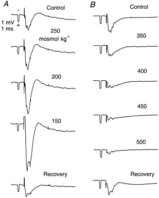
Field potentials recorded in cortical layer III in ACSF with different osmolalities

A, hypotonic series. Osmolalities shown on records. Note large increase in negativity of potentials with diminished osmolality. B, hypertonic series, osmolalities shown on records. Note decrease in negativity of potentials with increased osmolality. At 500 mosmol kg⁻¹ only a small presynaptic volley remains but postsynaptic response is restored when normal ACSF is applied (recovery). For both A and B, control and recovery ACSF were 305 mosmol kg⁻¹. Responses recorded at 25 min after osmolality changed. Same time and voltage calibration (shown in first record of A series) for all records. Each record was the average of four successive stimuli applied at the border of white matter and layer VI. Further details in Methods and Results.

Figure 1B shows results in a sequence of hyperosmotic solutions. The control record shows again the typical negative field potential in an ACSF of 305 mosmol kg⁻¹. As the solutions were changed through 350, 400, 450 and 500 mosmol kg⁻¹, the field potentials diminished, also seen by other investigators (Rosen & Andrew, 1990; Križaj et al. 1996; Tao, 1999). The reduction was probably caused both by an increase in the volume of the ECS (see later) and by a reduction in excitability. Upon return to isotonic medium, the evoked responses recovered to levels almost identical to control values.

Diffusion curves

Having established the viability of the slices under osmotic stress, the diffusion experiments are now presented. A sequence of diffusion curves in normal and in the most hypotonic ACSF is shown in Fig. 2A. There are four control records in 305 mosmol kg⁻¹ ACSF followed by four in 150 mosmol kg⁻¹ and then four after returning to 305 mosmol kg⁻¹ solution. Note that the records were taken with a greater time interval between them than shown in the figure to allow for the changed solution to equilibrate and baseline concentrations to stabilise. Figure 2A shows the dramatic increase in amplitude in the most hypotonic ACSF, 150 mosmol kg⁻¹, the small rise in baseline is due to the constant application of a forward bias current through the ionophoresis electrode (see Methods). It is also evident that the curves taken after the return to normal ACSF are slightly smaller than control values.

Figure 2.

Effects of osmotic challenges on diffusion curves

A, challenge with 150 mosmol kg⁻¹ ACSF. Sequence of four control diffusion records in 305 mosmol kg⁻¹ medium followed by four in 150 mosmol kg⁻¹ medium and finally four more records after return to 305 mosmol kg⁻¹ medium. Each record consisted of a 10 s baseline followed by the application of the ionophoretic current for 50 s causing the concentration of extracellular TMA⁺ ([TMA⁺]) to increase and then fall after the cessation of the current; the total duration of each individual record was 80 s. The interval between records was longer than that illustrated to permit baseline concentration to stabilise. For all records in A, r = 106 μm, n_t = 0.44. Average results for initial four control records were, λ = 1.67, α = 0.27, k’ = 0.020 s⁻¹; for the curves in hypotonic medium, λ = 1.80, α = 0.10, k’ = 0.016 s⁻¹; for the four records on return to control medium, λ = 1.57, α = 0.34, k’ = 0.015 s⁻¹. B, effect of challenge with 500 mosmol kg⁻¹ ACSF. The experiment was similar to that illustrated in A, except that hypertonic medium was used here. Sequence of four control records in 305 mosmol kg⁻¹ medium followed by four in 500 mosmol kg⁻¹ medium and finally four more records after return to 305 mosmol kg⁻¹ medium. For all records in B, r = 132 μm, n_t = 0.29. Average results for initial four control records were, λ = 1.77, α = 0.20, k’ = 0.024 s⁻¹; for the four curves in hypertonic medium, λ = 1.72, α = 0.37, k’ = 0.018 s⁻¹; for the four records on return to control medium, λ = 1.88, α = 0.13, k’ = 0.017 s⁻¹. In this and the subsequent figure, all concentrations are linear, derived from the ion-selective microelectrode (ISM) calibration. ○, ▪ and ▵ indicate curves shown in Fig. 3.

Figure 2B shows diffusion curves in control medium and in the most hypertonic ACSF, 500 mosmol kg⁻¹, with a similar protocol sequence to that displayed in Fig. 2A. In contrast to the case with hypotonic solution, the application of the hypertonic medium reduced both the amplitude and baseline level of the diffusion curves. After return to normal medium there was a distinct enhancement of amplitude, or ‘overshoot’, compared to control.

Three selected records, marked with symbols (○, ▪ or ▵) from each of the experiments shown in Fig. 2A and B are displayed in greater detail in Fig. 3. In panels 3A and B the curves show, control, osmotically challenged and recovery, plotted as changes in concentration from baseline, ΔC, so that the effect of bias current is removed. The fitted theoretical curve derived from eqn (1) is superimposed on each experimental curve and it is evident that they are indistinguishable. To appreciate the influence of λ on the curve shape, panels 3C and D show the normalised curves derived from eqn (3). The differences in curve shape reflect the differences in λ but it is clear that α is the main factor accounting for large amplitude differences seen in panels 3A and B (and Fig. 2).

Figure 3.

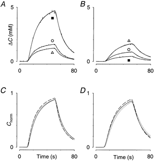
Detailed comparison of diffusion curves shown in Fig. 2

A, three curves taken from hypotonic series in Fig. 2A (indicated by ○ for control, ▵ for recovery and ▪ for value in hypotonic medium). In all three cases original data and curve fitted with eqn (1) are superimposed. To allow detailed comparison, the effect of the different baselines has been removed by plotting ΔC (concentration minus baseline). B, series in hypotonic medium taken from Fig. 2B. Same conventions as in A. The overshoot in the recovery medium is seen here. C, to understand how the differences in amplitude come about this panel uses a normalised plot of fitted curves according to eqn (3) that removes the influence of the changing volume fraction, α, leaving only the effect of tortuosity, λ, and clearance, k’. This panel corresponds to records in A. Control record, dashed line; 150 mosmol kg⁻¹, continuous line; recovery record, dotted line. D, the normalised versions of the records in B. Control record, dashed line; 500 mosmol kg⁻¹, continuous line; recovery record, dotted line. It is clear from C and D that most of the differences in the amplitudes of the curves are removed by the normalisation procedure, showing that amplitude is governed by α. The effects of λ and k’ are to alter the shapes of the curves slightly.

Sequences of records of the type shown in Figs 2A and B were made for all the different osmolalities used and D*, λ, α and k’ were obtained by fitting eqn (1) to the experimental data.

Measurements of D*, λ and α

Table 1 summarises all the data from our experiments, including both osmotic challenge and recovery. The results of the challenge are depicted graphically in Fig. 4. The recovery data were more variable because of the varying periods of osmotic stress and are included in Table 1 for completeness but are not considered in detail. The values of D* have been converted to tortuosities, using the relation: λ =√(D/D*), to facilitate later analysis and comparison with other studies. The required value of D was determined from eqn (4) to be 1.24 × 10⁻⁵ cm² s⁻¹ at 34 °C. The results in Table 1 confirmed that λ increased from a value of 1.69 ± 0.01 (n = 42, mean ± s.e.m.) in normal solution to 1.86 ± 0.01 (n = 12) in hypotonic 150 mosmol kg⁻¹ ACSF. In contrast, when tonicity was increased to 350 mosmol kg⁻¹, λ fell slightly to 1.67 ± 0.01 (n = 16) and then remained essentially constant. When the slice was returned to normal medium from hypotonic levels, it reached a more or less stable level, close to control levels, although there was some variation as a result of the stress. In contrast, when the slice returned from hypertonic to normal medium, a substantial overshoot occurred with λ reaching 1.91 ± 0.03 (n = 16) after exposure to 500 mosmol kg⁻¹ ACSF.

Table 1.

Diffusion parameters under osmotic challenge and after recovery in control ACSF

	Challenge				Recovery
ACSF osmolality mosmol kg−1	D* (10−6 cm2 s−1)	λ	α	n	D* (10−6 cm2 s−1)	λ	α	n
150	3.58 ± 0.05	1.86 ± 0.013	0.119 ± 0.006	12	4.58 ± 0.11	1.65 ± 0.021	0.346 ± 0.018	12
200	3.74 ± 0.05	1.82 ± 0.012	0.121 ± 0.005	20	4.18 ± 0.09	1.73 ± 0.019	0.318 ± 0.016	14
250	4.09 ± 0.05	1.74 ± 0.011	0.158 ± 0.008	11	4.47 ± 0.09	1.67 ± 0.018	0.234 ± 0.011	8
305†	4.34 ± 0.04	1.69 ± 0.009	0.240 ± 0.006	42	—	—	—	—
350	4.45 ± 0.04	1.67 ± 0.007	0.265 ± 0.006	16	4.29 ± 0.04	1.70 ± 0.009	0.216 ± 0.003	22
400	4.43 ± 0.06	1.67 ± 0.014	0.289 ± 0.012	15	3.89 ± 0.07	1.79 ± 0.008	0.202 ± 0.006	16
450	4.43 ± 0.06	1.68 ± 0.012	0.349 ± 0.022	9	3.65 ± 0.06	1.84 ± 0.014	0.205 ± 0.010	9
500	4.38 ± 0.06	1.68 ± 0.012	0.420 ± 0.015	18	3.43 ± 0.11	1.91 ± 0.031	0.185 ± 0.010	16

^†Control values. ACSF, artificial cerebrospinal fluid

^D*effective diffusion coefficient

λ, tortuosity; α, volume fraction; n, number of observations.

Figure 4.

Comparison of behaviour of λ measured with TMA⁺ and 3000 M_r dextran with behaviour of α (measured with TMA⁺)

Dextran data calculated from Tao (1999). Tortuosity measured with both molecules increases linearly as osmolality decreases below control value (305 mosmol kg⁻¹), but the slope measured with the larger molecule (dextran) is greater than that measured with the smaller (TMA⁺). In hypertonic ACSF, the value of λ measured with both molecules quickly reaches a constant value, λ₀ = 1.67. In contrast, α varies smoothly and monotonically with osmolality, decreasing in hypotonic ACSF and increasing in hypertonic medium. Further discussion in the text.

The average values of α for each osmotic challenge are shown in Table 1 and Fig. 4. They reveal that α decreased as tonicity was lowered, reaching a minimum value of 0.119 in 150 mosmol kg⁻¹ ACSF. The value of α increased as tonicity rose, to a maximum value of 0.420 in 500 mosmol kg⁻¹ solution. In normal medium, α was 0.240. When slices were returned to normal medium after osmotic challenge, the changes in α approximately mirrored the original changes; overshooting after hypotonic challenge in 150 mosmol kg⁻¹ solution to α = 0.346 and undershooting to α = 0.185 after hypertonic challenge in 500 mosmol kg⁻¹ ACSF.

TMA⁺ clearance

The analysis of the TMA⁺ diffusion curves, in addition to providing D* and α, also estimates k’ (s⁻¹), the clearance of TMA⁺. While the term ‘uptake’ has been commonly used, this parameter actually represents the loss of TMA⁺ from the ECS. The TMA⁺ may enter cells but in vivo it may also be lost across the blood-brain barrier while in a slice preparation, as used here, the TMA⁺ may be washed out into the surrounding bathing medium. From the control data we obtained k’ = 0.019 ± 0.001 s⁻¹, n = 42. The results in the different osmotic solutions showed no significant trends so the data were averaged to give k’ = 0.012 ± 0.001 s⁻¹, n = 101. Similarly, there was no trend evident in the recovery values and the data were again averaged to give k’ = 0.012 ± 0.001 s⁻¹, n = 97. The means under osmotic stress and recovery were not different but both differed from the mean in control ACSF (Student's t test, P < 0.01). This suggests that the imposition of osmotic stress, in either direction, may reduce k’, perhaps by altering the amount of TMA⁺ reaching the perfused surfaces of the slice.

Water content

A set of separate experiments was done in normal ACSF solution (305 mosmol kg⁻¹) and in solutions at the extremes of the osmotic range (150 and 500 mosmol kg⁻¹) to determine water content. There were two reasons for this analysis. First, to discover how water moved between extracellular and intracellular compartments and second, to estimate the dimensional change in the slice. This estimate enabled the maximum error in the electrode spacing to be calculated. Table 2 and Fig. 5 provide the results.

Table 2.

Water content after 30 min of osmotic challenge

ACSF osmolality (mosmol kg−1)	ω ( %)	n	α	(mi+me)/md	mi/md	me/md	x′/x ( %)
150	87.46 ± 0.16	3	0.12	7.00	6.04	0.96	108
305†	84.06 ± 0.26	9	0.24	5.28	3.77	1.51	100
500	83.09 ± 0.13	3	0.42	4.92	2.43	2.49	98

^†Control values. ACSF, artifical cerebrospinal fluid

ω, water content per wet-weight; n, number of observations; α, volume fraction; m_i mass intracellular water; m_e, mass extracellular water; m_d mass dry solids; x′, linear dimension of slice under osmotic stress; x, linear dimension of slice.

Figure 5.

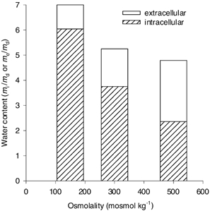
Distribution of water in normal and osmotically challenged slices

Cumulative bar graph shows intracellular, extracellular and total water (sum of the two) in normal (305 mosmol kg⁻¹), hypotonic (150 mosmol kg⁻¹) and hypertonic (500 mosmol kg⁻¹) ACSF, based on data in Table 2. The figure shows that in hypertonic medium the water content of the ECS exceeds that of the intracellular compartment. Note that the total water content of the slice increases in hypotonic medium and decreases slightly in hypertonic medium.

In the hyperosmolar solution the main effect was a movement of water from intra- to extracellular space with little change in total water content and the error in electrode spacing (x′/x, Table 2) would be no more than 2 %. Thus the ‘plateau’ effect is not caused by undue change in the size of the slice or consequent changes in electrode spacing. In the hypotonic solution, water moves from extra- to intracellular space but the tissue also gains water resulting in a possible error in electrode spacing of 8 %. This spacing change could have a small effect on the results in the most extreme solution but will not affect the overall results.

Quantitative description of λ and α as a function of osmolality

The major focus of this paper is to compare the behaviour of λ and α during osmotic challenge. To facilitate this, it is useful to quantify the relationships. Figure 4 shows that a linear regression fitted the set of λ-values corresponding to 150, 200, 250 and 305 mosmol kg⁻¹ while the λ-values for 350, 400, 450 and 500 mosmol kg⁻¹ could be represented by a constant.

This procedure yields the equations:

and

(12)

where Π is the osmolality in mosmol kg⁻¹. The r² value for the linear regression was 0.97.

The volume fraction was described by a second order regression (Fig. 4):

(13)

and the r² value for the second order regression was 0.98.

Figure 4 also shows a set of data derived by Tao (1999) in a study of the effective diffusion coefficient (D*_DEX) of 3000 M_r fluorescent dextran in neocortical slices using the IOI method (Nicholson & Tao, 1993). The D*_DEX values obtained by Tao (1999) have been converted to tortuosities using a D value of 2.12 × 10⁻⁶ cm² s⁻¹ at 34 °C, measured previously in 0.3 % agarose gel, dissolved in 150 mm NaCl (Nicholson & Tao, 1993), together with further measurements made during the course of subsequent work. As with TMA⁺, it is evident that the values of λ obtained with dextran in hypotonic ACSF can be represented by a straight line while values in hypertonic solutions can be fitted by the same constant as the TMA⁺ data. The actual values obtained were:

and

(14)

with an r² value of 0.99 for the regression. Looking at the hypotonic regime, it is evident that λ measured with dextran increases more rapidly with diminishing osmolality than when measured with TMA⁺. Both lines intercept at λ = 1.67 and an osmolality of 340 mosmol kg⁻¹.

The implications of these results can be visualised by generating a set of diffusion curves using eqn (1) with the baseline given by eqn (2). The experimental data do not lend themselves to this representation because r, n_t and k’ all vary slightly from one experiment to another. Figure 6 shows a set of curves generated from eqn (1) with baseline given by eqn (2) and values of λ and α obtained from eqns (12) and (13), respectively. The individual curves are projected on the [TMA]-Time plane and used to form a surface as a function of osmolality and time. It is evident that the large amplitude of the curve seen in hypotonic solutions drops quickly as tonicity increases, due primarily to the increasing α. As the value of osmolality passes through the control value, the magnitudes of the curves continue to fall slightly because of the continuing rise in α. There are subtle changes in the shapes of the curves, caused by the changes in λ, but these are not evident by inspection.

Figure 6.

Simulation of effect of osmolality on diffusion curves

Because electrode spacing, transport number and clearance vary slightly between experiments, the original curves cannot be easily compared so values of λ and α were derived from eqns (12) and (13). These values were then inserted in eqn (1) to generate the curves shown in this figure. Equation (2) was used with a bias current of 20 nA to give the baseline for the first 10 s, then a main current of 100 nA was applied in the interval 10–60 s. A constant clearance of k’ = 0.02 s⁻¹ was used, the electrode spacing was 100 μm and the transport number was n_t = 0.3. The shape of the concentration surface changes dramatically as osmolality increases as seen when every fourth concentration curve is projected on the [TMA⁺]-Time plane (cf. Figs 2 and 3).

DISCUSSION

This study focuses on the relation between λ and α, employing osmotic stress as a means of changing the parameters. There is a roughly inverse relation between λ and α, as seen in an earlier study on the cerebellum of the turtle (Križaj et al. 1996). But the detailed behaviours of the two parameters clearly differ. Volume fraction follows a smooth, monotonic curve that is well fitted by a second-order regression through both hypotonic and hypertonic ACSF solutions. In contrast, tortuosity obeys a linear relation in hypotonic solution and then becomes constant in hypertonic media. Before discussing these results it is pertinent to compare our data in slices to other diffusion studies on the cortex and to briefly consider volume regulatory processes in the slice.

Comparison of λ, α and k′ with values from other studies

The average value of λ that we measured in this study in normal (305 mosmol kg⁻¹) ACSF was 1.69 and the average value of α was 0.24. In previous studies on cortical slices, the values obtained were: λ = 1.62 and α = 0.18 (Pérez-Pinzón et al. 1995) and λ = 1.66 and α = 0.25 (Hrabětová & Nicholson, 2000). Most values that have been obtained in rat cortex in vivo tended to have slightly lower values of λ, ranging from 1.5–1.63, while a ranged from 0.18–0.23 (Cserr et al. 1991; Lehmenkühler et al. 1993; Voříšek & Syková, 1997b).

It appears that the control values of α in our slices are similar to those in the intact animal but our control values of λ are slightly larger (as reported also in the independent study by Hrabětová & Nicholson, 2000). One hypothesis that might account for this is that slices take up a certain amount of water during the initial incubation period after they are cut and much of this enters intracellular compartments (Hrabětová et al. 2002). It is likely that glia swell or undergo some astrogliosis and recent studies have suggested that such glial behaviour may lead to the formation of diffusion barriers and an increase in λ without altering α (Syková et al. 1996, 1999). An alternative explanation may be that the loss of TMA+ from the slice surface is not exactly described by the conventional clearance term in the diffusion equation and this can lead to a slight overestimate of λ (C. Nicholson & S. Hrabětová, unpublished observations).

It is noteworthy that a set of limiting values can be derived from eqns (12) and (13) as osmolality is reduced to zero, i.e. as Π→ 0. Equation (12) implies that, under these conditions, λTMA → 2.02 while eqn (13) implies that α→ 0.048. These limiting values of λTMA and α are almost identical to the values (λ = 2.0, α = 0.06) seen under severe ischaemic conditions in the intact animal (Voříšek & Syková, 1997b).

Clearance (k′) measured in normal ACSF in the present study, using submerged slices, averaged 0.019 s⁻¹ whereas values in previous submerged slice studies ranged between 0.013–0.016 s⁻¹ in hippocampus and 0.005 s⁻¹ in cortex (Perez-Pinzon et al. 1995) and 0.012 s⁻¹ in cortex (Hrabětová & Nicholson, 2000). Values recorded in the mature cortex in vivo ranged between 0.003–0.007 s⁻¹ (Cserr et al. 1991; Lehmenkühler et al. 1993; Voříšek & Syková, 1997b). It is likely, however, that ‘clearance’ is primarily mediated by loss across the blood–brain barrier in vivo while in vitro the loss occurs mainly through TMA+ entering the flowing ACSF at the surfaces of the slice (Nicholson et al. 2000). The effect of such washout is quite dependent on electrode position and flow conditions therefore the in vitro and in vivo values of k’ are not directly comparable.

Volume regulation in the cortical slice

On the time-scale of our measurements, we did not see any evidence of volume regulation (i.e. no regulatory volume increase or decrease) in our slices. This is consistent with our earlier study on the isolated turtle cerebellum (Križaj et al. 1996) and the study by Andrew et al. (1997). Andrew et al. (1997) using hippocampal slices and both light scattering and resistance measurements, showed no volume regulation when ACSF was diluted to reach an osmolality some 120 mosmol kg⁻¹ less than normal ACSF or when osmolality was increased by 40 mosmol kg_1 by adding mannitol. In contrast, Chebabo et al. (1995) saw some evidence of volume regulation over a period of an hour using hypotonic solutions with reduced NaCl, and a variant of the TMA+ method, in hippocampal slices. We note, however, that Chebabo et al. (1995) used an interface chamber while we used a submersion chamber for our diffusion studies. A subsequent study by Aitken et al. (1998), using freshly isolated hippocampal neurons found no consistent evidence of volume regulatory changes.

Reduction of osmolality invariably means either removing NaCl or diluting the entire ACSF but hypertonic solutions can either be achieved by adding more NaCl, as we did here, or by adding a substance not found in brain tissue, as did Andrew et al. (1997). There is no doubt that complex issues are involved because alteration of NaCl not only affects osmolality but is likely to influence active transport. The overshoot and undershoot in concentration after return to control ACSF (Figs 2 and 3; Table 1) suggest the presence of such mechanisms. In this study, however, we were using NaCl modification as a way of manipulating the geometry of the ECS and the absence of volume regulation during the osmotic challenge was fortuitous for our studies, since it provided stability over a sufficient time to make several repeatable measurements.

Comparison of λ values measured with TMA⁺ and dextran

It is of considerable interest to compare the behaviour of λ, obtained here using TMA⁺, with the study by Tao (1999) using a different molecule, 3000 M_r dextran, and different measuring technique (IOI) but under identical experimental conditions to those used here. When osmolality was reduced to a value of 150 mosmol kg⁻¹, λ measured with both molecules increased linearly but the slope was greater with dextran than with TMA⁺ (Fig. 4). These results suggest that, as the ECS shrinks, 3000 M_r dextran experiences more hindrance than does the smaller TMA⁺. As the osmolality increased beyond the isotonic level, the tortuosities measured with both molecules fell, but since the slopes were different, they intersected at a value of about 1.67, corresponding to 340 mosmol kg⁻¹. Thereafter, as tonicity increased to 500 mosmol kg⁻¹, both tortuosities remained essentially constant. In contrast, α (measured with TMA⁺) decreased in hypotonic medium and increased in hypertonic medium.

The difference in slopes of the λvs. osmolality curve in hypotonic medium, and the fact that the lines only intercept at 340 mosmol kg⁻¹, accounts for why the value of λ measured with TMA⁺ and dextran differ at normal osmolality (305 mosmol kg⁻¹). This may also explain the increased values of λ measured with larger dextrans in normal ACSF (Nicholson & Tao, 1993). These results also show that in the region of normal osmolality (305 mosmol kg⁻¹), λ is slightly above the plateau and therefore quite sensitive to the actual osmolality used in a particular study, so different investigators might obtain different values depending on the conditions of their preparations or formulation of their ACSF.

Geometrical tortuosity

The convergence of the values of λ, measured with both TMA⁺ and dextran, to a constant value, λ₀ = 1.67, in hypertonic media is very interesting. Since α is increasing during the hypertonic stress, it is assumed that the spaces between cells are increasing, but nevertheless, λ does not change. This result was so striking that it prompted us to develop a new model of the ECS under hypertonic challenge (Chen & Nicholson, 2000). The key feature of this model is that cells not only shrink as osmolality increases but also change shape. The shape changes cause the cells to become more rounded and result in the formation of residual spaces or ‘lakes’ at the interstices between some cells. When diffusing molecules enter such spaces they are temporarily trapped there before moving out into the adjacent clefts, resulting in an increased transit time and hence an increase in tortuosity that offsets the overall tendency for λ to diminish as osmolality falls. A related explanation has been given for certain behaviours of drug molecules in macroporous polymers (Siegel & Langer, 1990). This ‘plateau’ behaviour in λ can only persist over a limited osmotic range; eventually as the increased spaces surround all the cells they are no longer isolated pockets of residual space and λ must progress inexorably towards a final value of one, the free medium value.

Because, according to the above explanation, the value of λ₀ depends only on the structure or geometry of the ECS, it is appropriate to call it the ‘geometrical tortuosity’ i.e. this value does not include any contribution from interstitial viscosity, finite molecular size or other factors. The idea of a geometrical tortuosity was employed by Rusakov & Kullmann (1998) who used a model to calculate a value of either 1.40 or 1.57 for brain tissue, depending on whether a radial geometry or rectangular system was used. While some experimental data are close to the value estimated by Rusakov & Kullmann (1998), our experimental value for λ₀ is larger than either of these estimates. Furthermore, the definition of tortuosity that we use (Nicholson & Phillips, 1981) is inherently independent of the co-ordinate system used to measure it. Thus it is probable that the parameter calculated by Rusakov & Kullmann (1998) is not identical to one we measured (for additional discussion see Chen & Nicholson, 2000).

It may also be that a purely geometrical explanation will account for the increases in λ that occur with decreasing osmolality. For example, if the reduction in ECS volume leads to the formation of dead-end pores (Goodknight & Fatt, 1961) then tortuosity can be expected to increase (see Hrabětová & Nicholson 2000; Hrabětová et al. 2002 for another application of this conjecture). The explanation for this part of the λ–α curve, however, may reside in the properties of the extracellular matrix. This matrix consists of long-chain glycoproteins and glycosaminoglycans, including hyaluronate (Bignami et al. 1993; Ruoslahti, 1996) and a particular form of the matrix called the perineuronal net (Celio & Blumcke, 1994). The matrix might be sufficiently dense to form an obstructive polymer, which would restrict the diffusion of molecules (Ogston & Sherman, 1961). The swelling cells could compress the matrix, making it more obstructive and effectively increasing the viscosity of the interstitial medium. This possibility was explored recently in the paper by Rusakov & Kullman (1998), using previously published data from our laboratory and that of Dr E. Syková. It is impossible here to consider in detail the theoretical model proposed in that paper but we note that several attempts have been made over the years to account for the obstructive effects of large quasi-stationary macromolecules on the diffusion of small molecules (e.g. Wang, 1954, Ogston & Sherman, 1961; Clark et al. 1982; Johnson et al. 1996). This remains a fascinating area for further experimental and theoretical investigation.

Archie's Law

A relation was derived empirically by Archie (1942) in a quest to relate the impedance properties of geological formations to the presence of oil deposits. Archie's results may be stated in the form of a power law:

(15)

In the original form of eqn (15), γ = 1 (required if the relation is going to satisfy λ = 1, α = 1) and β = 0.5-0.7. Archie's Law has been used in the practical applications of porous media theory but attempts to derive the model theoretically have met with limited success (e.g. Sen et al. 1981) because all models require some assumptions about the underlying structure. In the context of the ECS, three papers have discussed Archie's Law (Nicholson & Rice, 1986; Lipinski, 1990; Lundbæk & Hansen, 1992). More recently, studies with MRI and NMR have returned to Archie's Law (Latour et al. 1994; Pfeuffer et al. 1998). Although the true test of a power law relation is to look for conformity over several orders of magnitude, it is nevertheless evident that even the limited data shown in Fig. 4 do not conform very well to this law. A power law can be fitted approximately to the λ-α values in the interval [0, 340] mosmol kg⁻¹, using eqns (12) and (14) but the fit gives γ = 0.72 and β = 0.23; furthermore there is no fit to the λ-α values in the interval [340, 500] mosmol kg⁻¹.

Independence of tortuosity and volume fraction

The disparity between the behaviour of λ and α implies an independence of the two parameters. Tortuosity and volume fraction are very different entities. Volume fraction is simple to define and, at least in principle, simple to measure. For example, with adequate fixation techniques, α can be measured directly from an electron micrograph (Bondareff & Pysh, 1968; Cragg, 1979) because the ratio of intracellular to extracellular spaces is the same in a two-dimensional section as in the three-dimensional volume, according to the Delisse Principle (Underwood, 1970). In contrast, tortuosity is a more elusive concept. It is thought of as a measure of the increased hindrance encountered by particles wandering through a medium containing obstructions. This leads to the idea of comparing random walks in a free medium to walks in the obstructed medium and, by extension from the microscopic domain to the macroscopic, comparing diffusion coefficients under the two circumstances (Nicholson & Syková, 1998). There are, however, many subtle issues in going from the geometric picture of hindered random walks to defining λ as the square root of the ratio of two diffusion coefficients (Chen & Nicholson, 2000; Nicholson, 2001). In addition, non-geometric factors such as interstitial viscosity and ratio of molecular size to channel width may come into play (Rusakov & Kullmann, 1998).

Other studies substantiate the independence of tortuosity and volume fraction. During postnatal development in the rat cortex (Lehmenkühler et al. 1993), λ remains constant but α changes from 40 to 20 % and measurements in the cortex of developing rats exposed to X-irradiation show that λ actually can increase while α rises (Syková et al. 1996).

The findings of this study are relevant to several broader issues. They reveal that there are complex constraints on the diffusion of molecules in the ECS that warrant further investigation. The results confirm that osmotic stress, using NaCl substitution, is an effective and reliable tool for modifying the ECS. In the context of pathophysiology, the results are not only applicable to situations where the brain is subject to osmotic challenge but also to ischaemic or anoxic conditions.

REFERENCES

- Agnati LF, Fuxe K, Nicholson C, Syková E, editors. Progress in Brain Research. Vol. 125. Amsterdam: Elsevier; 2000. Volume Transmission Revisited. [Google Scholar]
- Aitken PG, Borgdorff AJ, Juta AJ, Kiehardt DP, Somjen GG, Wadman WJ. Volume changes induced by osmotic stress in freshly isolated rat hippocampal neurons. Pflügers Archiv. 1998;436:991–998. doi: 10.1007/s004240050734. [DOI] [PubMed] [Google Scholar]
- Andrew RD, Lobinowich ME, Osehobo EP. Evidence against volume regulation by cortical brain cells during acute osmotic stress. Experimental Neurology. 1997;143:300–312. doi: 10.1006/exnr.1996.6375. [DOI] [PubMed] [Google Scholar]
- Archie GE. The electrical resistivity log as an aid in determining some reservoir characteristics. Transactions of the American Institute of Mining, Metallurgical and Petroleum Engineers, Incorporated. 1942;146:54–62. [Google Scholar]
- Bignami A, Hosley M, Dahl D. Hyaluronic acid and hyaluronic acid-binding proteins in brain extracellular matrix. Anatomy and Embryology. 1993;188:419–433. doi: 10.1007/BF00190136. [DOI] [PubMed] [Google Scholar]
- Bondareff W, Pysh JJ. Distribution of the extracellular space during postnatal maturation of rat cerebral cortex. Anatomical Record. 1968;160:773–780. doi: 10.1002/ar.1091600412. [DOI] [PubMed] [Google Scholar]
- Bungay PM, Morrison PF, Dedrick RL. Steady-state theory for quantitative microdialysis of solutes and water in vivo and in vitro. Life Sciences. 1990;46:105–119. doi: 10.1016/0024-3205(90)90043-q. [DOI] [PubMed] [Google Scholar]
- Celio MR, Blumcke I. Perineuronal nets — a specialized form of extracellular matrix in the adult nervous system. Brain Research Reviews. 1994;19:128–145. doi: 10.1016/0165-0173(94)90006-x. [DOI] [PubMed] [Google Scholar]
- Chebabo SR, Hester MA, Jing J, Aitken PG, Somjen GG. Interstitial space, electrical resistance and ion concentrations during hypotonia of rat hippocampal slices. Journal of Physiology. 1995;487:685–697. doi: 10.1113/jphysiol.1995.sp020910. [DOI] [PMC free article] [PubMed] [Google Scholar]
- Chen KC, Nicholson C. Changes in brain cell shape create residual extracellular space volume and explain tortuosity behavior during osmotic challenge. Proceedings of the National Academy of Sciences of the USA. 2000;97:8306–8311. doi: 10.1073/pnas.150338197. [DOI] [PMC free article] [PubMed] [Google Scholar]
- Clark ME, Burnell EE, Chapman NR, Hinke JAM. Water in barnacle muscle. IV. Factors contributing to reduced self-diffusion. Biophysical Journal. 1982;39:289–299. doi: 10.1016/S0006-3495(82)84519-0. [DOI] [PMC free article] [PubMed] [Google Scholar]
- Cragg B. Brain extracellular space fixed for electron microscopy. Neuroscience Letters. 1979;15:301–308. doi: 10.1016/0304-3940(79)96130-5. [DOI] [PubMed] [Google Scholar]
- Cserr HF, Depasquale M, Nicholson C, Patlak CS, Pettigrew KD, Rice ME. Extracellular volume decreases while cell volume is maintained by ion uptake in rat brain during acute hypernatremia. Journal of Physiology. 1991;442:277–295. doi: 10.1113/jphysiol.1991.sp018793. [DOI] [PMC free article] [PubMed] [Google Scholar]
- Fenstermacher JD, Patlak CS, Blasberg RG. Transport of material between brain extracellular fluid, brain cells and blood. Federation Proceedings. 1974;33:2070–2074. [PubMed] [Google Scholar]
- Fuxe K, Agnati LF, editors. Advances in Neuroscience. Vol. 1. New York: Raven Press; 1991. Volume Transmission in the Brain. [Google Scholar]
- Goodknight RC, Fatt I. The diffusion time-lag in porous media with dead-end pore volume. Journal of Physical Chemistry. 1961;65:1709–1712. [Google Scholar]
- Hrabětová S, Chen KC, Masri D, Nicholson C. Water compartmentalization and spread of ischemic injury in thick-slice ischemia model. Journal of Cerebral Blood Flow and Metabolism. 2002;22:80–88. doi: 10.1097/00004647-200201000-00010. [DOI] [PubMed] [Google Scholar]
- Hrabětová S, Nicholson C. Dextran decreases extracellular tortuosity in the thick-slice ischemia model. Journal of Cerebral Blood Flow and Metabolism. 2000;20:1306–1310. doi: 10.1097/00004647-200009000-00005. [DOI] [PubMed] [Google Scholar]
- Johnson EM, Berk DA, Jain RK, Deen WM. Hindered diffusion in agarose gels: Test of effective medium model. Biophysical Journal. 1996;70:1017–1023. doi: 10.1016/S0006-3495(96)79645-5. [DOI] [PMC free article] [PubMed] [Google Scholar]
- Krizaj D, Rice ME, Wardle RA, Nicholson C. Water compartmentalization and extracellular tortuosity after osmotic changes in cerebellum of Trachemys scripta. Journal of Physiology. 1996;492:887–896. doi: 10.1113/jphysiol.1996.sp021354. [DOI] [PMC free article] [PubMed] [Google Scholar]
- Latour LL, Svoboda K, Mitra PP, Sotak CH. Time-dependent diffusion of water in a biological model system. Proceedings of the National Academy of Sciences of the USA. 1994;91:1229–1233. doi: 10.1073/pnas.91.4.1229. [DOI] [PMC free article] [PubMed] [Google Scholar]
- Lehmenkühler A, Syková E, Svoboda J, Zilles K, Nicholson C. Extracellular space parameters in the rat neocortex and subcortical white matter during postnatal development determined by diffusion analysis. Neuroscience. 1993;55:339–351. doi: 10.1016/0306-4522(93)90503-8. [DOI] [PubMed] [Google Scholar]
- Lipinski H-G. Monte-Carlo simulation of extracellular diffusion in brain tissues. Physics in Medicine and Biology. 1990;35:441–447. doi: 10.1088/0031-9155/35/3/012. [DOI] [PubMed] [Google Scholar]
- LundbÆk JA, Hansen AJ. Brain interstitial volume fraction and tortuosity in anoxia. Evaluation of the ion-selective micro-electrode method. Acta Physiologica Scandinavica. 1992;146:473–484. doi: 10.1111/j.1748-1716.1992.tb09449.x. [DOI] [PubMed] [Google Scholar]
- Nicholson C. Ion-selective microelectrodes and diffusion measurements as tools to explore the brain cell microenvironment. Journal of Neuroscience Methods. 1993;48:199–213. doi: 10.1016/0165-0270(93)90092-6. [DOI] [PubMed] [Google Scholar]
- Nicholson C. Diffusion and related transport mechanisms in brain tissue. Reports on Progress in Physics. 2001;64:815–884. [Google Scholar]
- Nicholson C, Chen KC, Hrabětová S, Tao L. Diffusion of molecules in brain extracellular space: theory and experiment. In: Agnati LF, Fuxe K, Nicholson C, Syková E, editors. Volume Transmission Revisited. Vol. 125. Amsterdam: Elsevier; 2000. pp. 129–154. Progress in Brain Research. [DOI] [PubMed] [Google Scholar]
- Nicholson C, Hounsgaard J. Diffusion in the slice microenvironment and implications for physiological studies. Federation Proceedings. 1983;42:2865–2868. [PubMed] [Google Scholar]
- Nicholson C, Phillips JM. Ion diffusion modified by tortuosity and volume fraction in the extracellular microenvironment of the rat cerebellum. Journal of Physiology. 1981;321:225–257. doi: 10.1113/jphysiol.1981.sp013981. [DOI] [PMC free article] [PubMed] [Google Scholar]
- Nicholson C, Rice ME. The migration of substances in the neuronal microenvironment. Annals of the New York Academy of Sciences. 1986;481:55–71. doi: 10.1111/j.1749-6632.1986.tb27139.x. [DOI] [PubMed] [Google Scholar]
- Nicholson C, Syková E. Extracellular space structure revealed by diffusion analysis. Trends in Neuroscience. 1998;21:207–215. doi: 10.1016/s0166-2236(98)01261-2. [DOI] [PubMed] [Google Scholar]
- Nicholson C, Tao L. Hindered diffusion of high molecular weight compounds in brain extracellular microenvironment measured with integrative optical imaging. Biophysical Journal. 1993;65:2277–2290. doi: 10.1016/S0006-3495(93)81324-9. [DOI] [PMC free article] [PubMed] [Google Scholar]
- Nicholson C, Tao L, Kume-Kick J. Constraints on the extracellular diffusion of molecules. Journal of Physiology. 1998;511:P8. [Google Scholar]
- Nicolay K, Braun KPJ, De Graaf RA, Dijkhuizen RM, Kruiskamp MJ. Diffusion NMR spectroscopy. NMR in Biomedicine. 2001;14:94–111. doi: 10.1002/nbm.686. [DOI] [PubMed] [Google Scholar]
- Norris DG. The effects of microscopic tissue parameters on the diffusion weighted magnetic resonance imaging experiment. NMR in Biomedicine. 2001;14:77–93. doi: 10.1002/nbm.682. [DOI] [PubMed] [Google Scholar]
- Ogston AG, Sherman TF. Effects of hyaluronic acid upon diffusion of solutes and flow of solvent. Journal of Physiology. 1961;156:67–74. doi: 10.1113/jphysiol.1961.sp006658. [DOI] [PMC free article] [PubMed] [Google Scholar]
- Pérez-Pinzón MA, Tao L, Nicholson C. Extracellular potassium, volume fraction, and tortuosity in rat hippocampal CA1, CA3, and cortical slices during ischemia. Journal of Neurophysiology. 1995;74:565–573. doi: 10.1152/jn.1995.74.2.565. [DOI] [PubMed] [Google Scholar]
- Pfeuffer J, Dreher W, Syková E, Leibfritz D. Water signal attenuation in diffusion-weighted 1H NMR experiments during cerebral ischemia: influence of intracellular restrictions, extracellular tortuosity and exchange. Magnetic Resonance Imaging. 1998;16:1023–1032. doi: 10.1016/s0730-725x(98)00107-6. [DOI] [PubMed] [Google Scholar]
- Press WH, Flannery BP, Teukolsky SA, Vetterling WT. Numerical Recipes. UK: Cambridge University Press; 1986. [Google Scholar]
- Rosen AS, Andrew RD. Osmotic effects upon excitability in rat neocortical slices. Neuroscience. 1990;38:579–590. doi: 10.1016/0306-4522(90)90052-6. [DOI] [PubMed] [Google Scholar]
- Ruoslahti E. Brain extracellular matrix. Glycobiology. 1996;6:489–492. doi: 10.1093/glycob/6.5.489. [DOI] [PubMed] [Google Scholar]
- Rusakov DA, Kullmann DM. Geometric and viscous components of the tortuosity of the extracellular space in the brain. Proceedings of the National Academy of Sciences of the USA. 1998;95:8975–8980. doi: 10.1073/pnas.95.15.8975. [DOI] [PMC free article] [PubMed] [Google Scholar]
- Saltzman WM. Drug Delivery: Engineering Principles for Drug Therapy. Oxford: Oxford University Press; 2001. [Google Scholar]
- Saltzman WM, Radomsky ML. Drugs released from polymers: diffusion and elimination in brain tissue. Chemical Engineering Science. 1991;46:2429–2444. [Google Scholar]
- Sen PN, Scala C, Cohen MH. A self-similar model for sedimentary rocks with application to the dielectric constant of fused glass beads. Geophysics. 1981;46:781–795. [Google Scholar]
- Siegel RA, Langer RL. Mechanistic studies of macromolecular drug release from macroporous polymers. II. Models for the slow kinetics of drug release. Journal of Controlled Release. 1990;14:153–167. [Google Scholar]
- Syková E. The extracellular space in the CNS: its regulation, volume and geometry in normal and pathological neuronal function. Neuroscientist. 1997;3:28–41. [Google Scholar]
- Syková E, Svoboda J, Šimonová Z, Lehmenkühler A, Lassmann H. X-irradiation-induced changes in the diffusion parameters of the developing rat brain. Neuroscience. 1996;70:597–612. doi: 10.1016/0306-4522(95)00361-4. [DOI] [PubMed] [Google Scholar]
- Syková E, Vargová L, Prokopová Š, Šimonová Z. Glial swelling and astrogliosis produce diffusion barriers in the rat spinal cord. Glia. 1999;25:56–70. doi: 10.1002/(sici)1098-1136(19990101)25:1<56::aid-glia6>3.0.co;2-4. [DOI] [PubMed] [Google Scholar]
- Tao L. Effects of osmotic stress on dextran diffusion in rat neocortex studied with integrative optical imaging. Journal of Neurophysiology. 1999;81:2501–2507. doi: 10.1152/jn.1999.81.5.2501. [DOI] [PubMed] [Google Scholar]
- Underwood EE. Quantitative Stereology. MA, USA: Addison-Wesley, Reading; 1970. [Google Scholar]
- Voříšek I, Syková E. Evolution of anisotropic diffusion in the developing rat corpus callosum. Journal of Neurophysiology. 1997a;78:912–919. doi: 10.1152/jn.1997.78.2.912. [DOI] [PubMed] [Google Scholar]
- Voříšek I, Syková E. Ischemia-induced changes in the extracellular space diffusion parameters, K+, and pH in the developing rat cortex and corpus callosum) Journal of Cerebral Blood Flow and Metabolism. 1997b;17:191–203. doi: 10.1097/00004647-199702000-00009. [DOI] [PubMed] [Google Scholar]
- Wang JH. Theory of the self-diffusion of water in protein solutions. A new method for studying the hydration and shape of protein molecules. Journal of the American Chemical Society. 1954;76:4755–4765. [Google Scholar]