VALIDATION OF CFD PREDICTIONS OF FLOW IN A 3D ALVEOLATED BEND WITH EXPERIMENTAL DATA

Abstract

Verifying numerical predictions with experimental data is an important aspect of any modeling studies. In the case of the lung, the absence of direct in-vivo flow measurements makes such verification almost impossible. We performed computational fluid dynamics (CFD) simulations in a 3D scaled-up model of an alveolated bend with rigid walls that incorporated essential geometrical characteristics of human alveolar structures and compared numerical predictions with experimental flow measurements made in the same model by Particle Image Velocimetry (PIV). Flow in both models was representative of acinar flow during normal breathing (0.82 ml/s). The experimental model was built in silicone and silicone oil was used as the carrier fluid. Flow measurements were obtained by an ensemble averaging procedure. CFD simulation was performed with STAR-CCM+ (CD-Adapco) using a polyhedral unstructured mesh. Velocity profiles in the central duct were parabolic and no bulk convection existed between the central duct and the alveoli. Velocities inside the alveoli were ∼2 orders of magnitude smaller than the mean velocity in the central duct. CFD data agreed well with those obtained by PIV. In the central duct, data agreed within 1%. The maximum simulated velocity along the centerline of the model was 0.5% larger than measured experimentally. In the alveolar cavities, data agreed within 15% on average. This suggests that CFD techniques can satisfactorily predict acinar-type flow. Such a validation ensure a great degree of confidence in the accuracy of predictions made in more complex models of the alveolar region of the lung using similar CFD techniques.

INTRODUCTION

Many respiratory diseases are directly linked to air pollution and the deposition of particulate matter in the alveolar zone of the lungs (Dockery et al., 1993; Pope III et al., 2002; Pope, 1995; Schwartz and Dockery, 1992; Wilson, 1996). The specific pattern of particulate deposition in the airspaces is a key factor in determining the local doses and the subsequent redistribution and clearance of deposited particles. Deposition patterns are mainly affected by particle size and flow characteristics within the respiratory tract. To better understand the transport of aerosols in the complex flow field of the respiratory tract, both numerical modeling studies and in-vitro experiments have been performed. Computational fluid dynamics (CFD) modeling offers the flexibility of easily modifying parameters such as lung geometry, flow rates, particle sizes, and ventilation distribution. However, potential numerical errors and artifacts can lead to non-physiological CFD results. Experimental studies offer the advantage of physical realism; once the numerical model is experimentally validated, it is often more efficient to perform the parametric investigation numerically.

Many CFD studies have used complex realistic models of the lung (Harrington et al., 2006; Nowak et al., 2003; van Ertbruggen et al., 2005). These models provided detailed information on the flow field and deposition patterns within lung structures. However, the absence of direct in-vivo measurements in the lung made it almost impossible to validate numerical predictions from these models. In-vitro studies of the flow in lung structures have been performed by Particle Image Velocimetry (PIV), a non-intrusive technique that allows the measurement of instantaneous velocity fields. Ramuzat (2003) studied both steady and oscillating flow in a three-dimensional (3D) model of three successive generations of conducting airways. Karl and colleagues (2004) performed flow visualizations studies in a model of a straight alveolated duct that they used to verify CFD predictions, however no quantitative comparison was provided. Tippe and Tsuda (1999) used the PIV technique to study mixing processes in a model of a single expanding and contracting alveolus.

The aim of the present study, which modeled flow within a 3D alveolated bend, was three-fold: 1) develop a physical model that incorporates essential geometrical characteristics of alveolar structures in which experimental flow measurements could be obtained, 2) perform CFD simulations of the flow in a model that was the exact replica of the physical model, and 3) use the experimental data to verify the numerical predictions to validate the CFD approach. Such validation would ensure a great degree of confidence in the accuracy of CFD flow predictions made with more complex models of the acinar region of the lung for which experimental data may not be available.

MATERIAL AND METHODS

1. Model

We built a 3D alveolated bend (Fig. 1B) using a casting technique that utilized a low-melting point alloy (Low 158 – Alchemy Castings) for the core and a mixture of silicone and curing agent (Sylgard® 184) for the cast model. The silicon is transparent with a refractive index similar to the carrier fluid (silicon oil). These characteristics allowed for high quality optical access for the PIV measurements.

Figure 1.

Model of the alveolated bend. A: dimensions of the model (in mm). B: physical model used in the in-vitro study. C: model used in the CFD simulations.

The model consisted of two alveolated ducts joined by a 145° bend. Each duct was made of a cylinder (diameter=15mm) surrounded by three toroidal alveoli (outer diameter=30mm, height=5mm) regularly spaced by 2.5mm (Fig. 1). The model dimensions were about 50 times larger than those found in the alveolar region of the lung (Haefeli-Bleuer and Weibel, 1988; Weibel et al., 2005) to optimize experimental measurements.

2. Experimental setup

The experimental setup was built from an existing physiological flow facility available at the von Karman Institute for Fluid Dynamics (VKI) and is depicted in Fig. 2. A pump (4) filled a stagnation tank (5), which was connected with a tube (6) to the alveolar model (1). After having passed the model the silicon oil flowed over a flow meter (2) designed at the VKI to measure small flow rates. Flow was regulated by a ball valve located downstream of the model. The fluid dripped into a tank (3) before it was pumped back to the upper reservoir. To maintain a constant fluid level, the surplus of fluid in the compartment (5 left) overflowed into a second partition (5 right). The impeller (7) rotated at low speed to keep the fluid in motion to avoid that the tracer particles settle at the bottom of the reservoir. The facility covered a total height of about 3 meters to ensure the required flow rates.

Figure 2.

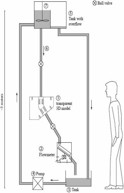
Experimental set-up. See text for details.

Silicone oil (ρ=970kg/m³, μ=1Pas) served as carrier fluid. A flow rate of 0.82 ml/s was used. It corresponded to a Reynolds number (Re) of 0.07 that was representative of typical flow conditions encountered at the level of the 21^st generation of the Weibel model (Weibel, 1963) where airways are fully alveolated. The difference in refractive index between the model and the fluid was negligible minimizing optical artifacts and reflections originating from the curved surfaces.

3. Particle Image Velocimetry (PIV)

PIV is a non-intrusive technique wherein a laser sheet is used to illuminate a flow field seeded with tracer particles. The positions of the particles are recorded with digital CCD cameras at specified time intervals. Data processing consists of determining the average displacement of the particles over a small interrogation region between two successive recorded images. Knowledge of the separation time between the images then permits the computation of two components of flow velocities.

In this study, 20 μm-diameter iron particles were used as tracers. Their small size made them almost neutrally buoyant, allowing for accurate tracing of the flow. Because the density of the fluid and of the particles was different, particles deviate from the streamlines. The particle size was chosen to minimize this effect while ensuring a particle surface area large enough to scatter sufficient light to provide a clear tracer pattern. The illumination and recording setup is depicted in Figure 3A. Large separation times and small flow velocities allowed the use of a continuous illumination source. A continuous Innova 70C Argon laser supplied the coherent light source with a wavelength of 514 nm. After passing the laser beam through an optical fiber it was shaped into a thin laser sheet by an optical assembly. The average sheet thickness was ∼1mm, illuminating a slice of the flow located at the symmetry plane. Reflections from the Plexiglas mountings at the top and bottom of the model caused the laser beam to intersect the model several times resulting in an uneven light intensity distribution inside the test section (Fig. 4A). To reduce these interferences, the laser sheet was tilted around the horizontal axis and an aperture was placed in front of the model (Fig. 4B). The scattered light intensities were recorded with a 12bit PCO Sensicam camera, equipped with a 50mm focal length Nikon lens. An imposed shutter time of 500−1000μs ensured the capture of ’frozen’ tracer patterns (Fig. 3B). The grabbing frequency was imposed by an external trigger connected to a host computer. The images had a typical resolution of 1280×640 pixel² and an average of 500 images was recorded.

Figure 3.

Image acquisition. A: experimental set-up showing the CCD camera (1) positioned in front of the model and the laser sheet (gray lines) formed through the optical assembly (2). B: Example of an instantaneous PIV recording where recirculation zone within the alveolar cavities can be clearly observed.

Figure 4.

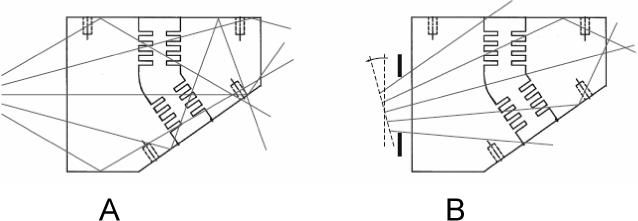
Illumination of the model by the laser sheet. A: horizontal illumination leading to reflections and crossovers. B: illuminations with reduced reflections obtained by tilting the laser sheet and passing it through as aperture.

Image processing was performed with a cross-correlation algorithm WiDIM (Scarano and Riethmuller, 2000) that uses a multigrid iterative approach. WiDIM allowed for high accuracy measurements as the second exposure interrogation-area could be displaced with sub-pixel accuracy. During the iterative procedure, the size of the interrogating windows was gradually reduced (the windows were halved in both directions), yielding a finer spatial resolution compared with one-step interrogation methods. Accordingly, the RMS of the displacement error was dramatically reduced to about 10⁻³ pixels. Furthermore WiDIM was designed to use overlapping windows allowing for increased sampling frequency.

When evaluating digital PIV recordings with conventional correlation algorithms, a sufficient number of particle images per interrogation window is required to perform a reliable cross-correlation. Typically, an average of ten particle images pairs suffice to ensure a reliable and accurate measurement. In the present experiments, because of the small dimensions of the alveoli, the number of tracers included in each interrogation windows was small. To overcome this problem, an ensemble averaging of the correlation fields was used over a number of successive doublets. This method was previously used in micro-PIV, where it was successfully applied over 50 doublets (Wereley et al., 2002). Such procedure reduced background noise and allowed for a better differentiation of the tracer patterns.

4. CFD simulation

We used CFD software STAR-Design v.4.02.016 (CD-Adapco) to build and mesh the alveolated bend geometry. We created a polyhedral unstructured mesh (Fig. 5A), with hexahedral cells for the core (Fig. 5B). Two subsurface layers (with prismatic cells) were inserted along the walls to increase the accuracy of the simulation where velocity gradients were the highest. The mesh was made of 320,000 cells, which was achieved by imposing a relative sizing of the mesh of 1%.

Figure 5.

Computational grid made of 320,000 nodes. A: polyhedral cells forming the outer surface of the model. B: Cross-section through the model showing the combination of unstructured and structured-hexahedral meshes. See text for details.

The mesh dependency of the solution was examined by solving the flow field for three mesh configurations made of 110,000, 194,000 and 320,000 cells, respectively. Velocity profiles were compared in several sections for the three mesh configurations. Up to 3.5% difference in the maximum velocity existed between the coarser and finer mesh and less than 0.2% difference existed between the two finer meshes, indicating that the finer mesh lead to mesh-independent solutions.

Flow field calculations were carried out by CFD code STAR-CCM+ v.1.08.018 (CD-Adapco). We simulated steady laminar flow for the same conditions as those used in the experimental study. A straight tube was added both at the inlet and outlet of the model to minimize the effect of the boundary conditions on the calculated flow. Since velocities in the model were extremely small (Re=0.07), we used a segregated flow model, with a second order convective scheme. Flow equations (one for each component of velocity and one for the pressure) were solved in a segregated manner, using the finite volume method. The linkage between the momentum and continuity equations was achieved with a predictor-corrector approach. The complete formulation can be described as using a collocated variable arrangement and a Rhie-Chow pressure-velocity coupling combined with SIMPLE algorithm.

A parabolic-shaped mass flow of 0.82 ml/s was imposed at the model inlet. A constant static pressure was imposed at the outlet. A no-slip boundary condition was applied at the wall boundaries. Convergence of the residuals was monitored and simulation was stopped when residuals had decreased by 5 orders of magnitude. Simulations ran on a Dell Precision workstation 530 MT (with 2 Intel Xeon processor 1.4 GHz, 2Gb Ram) under RedHat Linux Enterprise v.3, and took 270 iterations to reach the convergence threshold.

RESULTS AND DISCUSSION

1. Velocity field in the symmetry plane of the model

Figures 6A and 6B show velocity fields obtained by PIV and CFD, respectively. PIV data were obtained by correlation averaging over 50 images. The initial size of the interrogation windows was 80×80 pixels. The windows were gradually reduced to a final size of 20×20 pixels. A window overlapping of 50 % was used. A velocity vector could therefore be calculated every 10 pixels.

Figure 6.

Velocity field in the symmetry plane of the bend (Re=0.07). A: PIV data. B: CFD predictions.

In both the experimental and simulated velocity fields, two regions of high velocity upstream and downstream of the bend were identified. When approaching the curved bend, the flow decelerated due to the increase in cross-section, then accelerated when it entered the second alveolated duct. Velocity magnitudes inside the alveoli were about 2 orders of magnitude smaller than the mean velocity in the central duct. Velocity profiles in the central duct were parabolic. Assuming a Poiseuille profile, the maximum velocity in the central duct of section 2 (Fig. 6A) would be 9.28 mm/s for a flow rate of 0.82 ml/s. The maximum simulated velocity found along the centerline of the model in section 2 was 8.96 mm/s, 3% smaller than theory. Experimentally, the maximum velocity was 8.92 mm/s, 0.5% smaller than the simulated results

A quantitative comparison between experimental and simulated velocity profiles was performed at seven locations within the symmetry plane of the model (Figs. 7A-7G). These locations (sections 1−7) are defined in Figures 6A and 7H. Overall, experimental data agreed very well with CFD predictions. In the central duct, the largest differences were found in section 5 where PIV data were about 5% lower than CFD predictions. In the other sections, PIV and CFD data agreed on average within 1%.

Figure 7.

Comparison between CFD predictions (dashed line) and PIV measurements (dotted line) of velocity profiles along different sections of the model (panels A-H). In each of these panels, the orientation of the horizontal axes is such that length zero is on the outer side of the bend. The locations of the sections are defined in panel H.

While the geometry presented a converging-diverging channel to the flow, the presence of the alveolar cavities had a minimal effect on the flow in the central duct. In sections 2, 3, 6 and 7, the velocity profiles presented an almost perfect parabolic shape. When passing the alveolar cavities (sections 1 and 5), the flow slightly decelerated because of the larger cross-sectional area and the maximum velocity was reduced by ∼5% compared to that in the central duct of sections 2, 3, 6 and 7. Because the flow was dominated by viscous forces (small Re), the velocity profile regained its parabolic shape almost instantly. Indeed, the entrance length l_E, a measure of the distance required by the flow to be fully developed, is expressed by

$$\frac{I_E}{D}=0.06Re$$

for laminar flows (Munson et al., 1990), where D is the diameter of the central duct. In our case, l_E/D is 0.0042 and the velocity profile regained its parabolic shape in less than 0.1mm.

2. Flow in the alveolar cavities

Figures 8A and B shows the streamlines obtained in the symmetry plane by PIV and CFD, respectively. In most of the central duct, streamlines were parallel to the axial direction. Streamlines became curvilinear near the alveolar openings. A recirculation flow was positioned in the centre of each alveolus located in the straight portions of the model. These flow patterns were similar to those from previous numerical studies performed in alveolated ducts (Darquenne and Paiva, 1996; Federspiel and Fredberg, 1988; Harrington et al., 2006). Streamlines widened at the outer side of the bend due to the increase in the cross-sectional area, resulting in a skewed velocity profile in section 4 (Fig. 7D). Vortices were found in the corners of the alveolar cavity located in the outer side of the bend.

Figure 8.

Streamline patterns obtained in the symmetry plane (Re = 0.07). A: PIV data. B: CFD predictions.

A separation streamline at the mouth of the alveolar cavities was present, indicating only little convective exchange between flow in the central duct and the surrounding alveoli. The 3D CFD predictions showed non-planar streamlines patterns in the vicinity of and within alveolar cavities. For example, a 3D streamline that originated from the central duct can be seen appearing in the symmetry plane near the bend. Another 3D streamline seeming to hit the wall in the cavity surrounding the bend is actually disappearing from the plane.

Karl et al. (2004) studied low Re viscous flow in a straight alveolated duct and showed that the type of flow developing in the alveolar cavities was controlled by the ratio of the cavity depth to its width (cavity ratio, R_c). For the alveolar cavities in the straight portions of the model, R_c = 1.5. Karl et al. showed that for R_c> 2/3, the cavities were filled with one large recirculating region that was separated from the ductal flow by a streamline spanning the cavity opening. For the alveolus located in the outer side of the bend, R_c=0.4. For R_c<0.5, Karl et al. showed that flow in the cavities was characterized by two recirculating regions, one in each lower corner of the cavity, and that the ductal flow penetrated rather deeply in the cavity. These observations agree with our data.

A quantitative comparison between experimental and simulated velocity profiles within an alveolar cavity is shown in Figure 9. Velocity magnitudes were less than 0.1mm/s and on average two orders of magnitude smaller than the mean velocity in the central duct. To increase the resolution of the flow inside the alveoli, PIV data were recorded with a larger magnification than those shown in previous figures which led to larger experimental errors (∼5%). CFD predictions matched PIV data very well near the alveolar opening and near the bottom of the alveolus. CFD predictions were higher than PIV data in the middle section of the profile. For example, CFD prediction was 27% higher than PIV data at a distance of 4.5 mm from the bottom of the alveolar cavity (Fig. 9). Overall, CFD predictions were on average 15% higher than PIV data in the alveoli. Given higher experimental and numerical errors in the alveolar cavities compared to those in the central duct, we found a satisfactory agreement between both data sets.

Figure 9.

Comparison between CFD predictions (dashed line) and PIV measurements (dotted line) of velocity profiles within one alveolar cavity along section 5. The depth of the alveolus is 7.5 mm.

CONCLUSIONS

In the recent years, several CFD studies of aerosol transport in lung airspaces have been performed (Harrington et al., 2006; Nowak et al., 2003; van Ertbruggen et al., 2005) where accurate descriptions of the flow field were coupled to simplified tracking algorithms to determine deposition patterns within the models. The absence of direct in-vivo measurements in the lung made it almost impossible to validate numerical predictions from these models. In this study, we focused on the validation of the technique used to calculate flow in several previous studies (Darquenne, 2001; Darquenne, 2002; Darquenne and Paiva, 1996; Harrington et al., 2006). We used a test case model that was not intended to reflect the exact behavior of the human lung but that incorporated enough geometrical characteristics of alveolar structures to allow a realistic comparison.

It should however be noted that the absence of cyclic wall motion in the model is a major limitation in the simulation of acinar flows. This study is a first step in validating the use of CFD techniques to model pulmonary flows. A rigid-walled model still provides data with insight into the basic flow. These data will serve as a control set to emphasize changes in flow features brought by the inclusion of wall motion in a subsequent alveolar model. This is however beyond the scope of the present study.

Our results suggest that our computational model correctly predicts flow behavior in acinar structures: data agreed within 1% in most portions of the central duct and within 15% on average in the alveolar cavities. Our results suggest that flow may be accurately predicted in more complex models of the alveolar region of the lung that use similar CFD techniques.

References

- Darquenne C. A realistic two-dimensional model of aerosol transport and deposition in the alveolar zone of the human lung. J.Aerosol Sci. 2001;32:1161–1174. [Google Scholar]
- Darquenne C. Heterogeneity of aerosol deposition in a two-dimensional model of human alveolated ducts. J.Aerosol Sci. 2002;33:1261–1278. [Google Scholar]
- Darquenne C, Paiva M. Two- and three-dimensional simulations of aerosol transport and deposition in alveolar zone of human lung. J.Appl.Physiol. 1996;80:1401–1414. doi: 10.1152/jappl.1996.80.4.1401. [DOI] [PubMed] [Google Scholar]
- Dockery DW, Pope CA, III, Xu X, Spengler JD, Ware JH, Fay ME, Ferris F, Jr, Speizer FE. An association between air pollution and mortality in six US cities. New Eng.J.Med. 1993;329:1753–1759. doi: 10.1056/NEJM199312093292401. [DOI] [PubMed] [Google Scholar]
- Federspiel WJ, Fredberg JJ. Axial dispersion in respiratory bronchioles and alveolar ducts. J.Appl.Physiol. 1988;64:2614–2621. doi: 10.1152/jappl.1988.64.6.2614. [DOI] [PubMed] [Google Scholar]
- Haefeli-Bleuer B, Weibel E. Morphometry of the human pulmonary acinus. Anat.Record. 1988;220:401–414. doi: 10.1002/ar.1092200410. [DOI] [PubMed] [Google Scholar]
- Harrington L, Prisk GK, Darquenne C. Importance of the bifurcation zone and branch orientation in simulated aerosol deposition in the alveolar zone of the human lung. J.Aerosol Sci. 2006;37:37–62. [Google Scholar]
- Karl A, Henry FS, Tsuda A. Low Reynolds number viscous flow in an alveolated duct. Trans.ASME. 2004;126:420–429. doi: 10.1115/1.1784476. [DOI] [PubMed] [Google Scholar]
- Munson BR, Young DF, Okiishi TH. Fundamentals of fluid mechanics. John Wiley and Sons; 1990. [Google Scholar]
- Nowak N, Kakade PP, Annapragada AV. Computational fluid dynamics simulations of airflow and aerosol deposition in human lungs. Ann.Biomed.Eng. 2003;31:374–390. doi: 10.1114/1.1560632. [DOI] [PubMed] [Google Scholar]
- Pope CA, III, Burnett JC, Thun MJ, Calle EE, Krewski D, Ito K, Thurston GD. Lung cancer, cardiopulmonary mortality, and long-term exposure to fine particulate air pollution. J.A.M.A. 2002;287:1132–1141. doi: 10.1001/jama.287.9.1132. [DOI] [PMC free article] [PubMed] [Google Scholar]
- Pope AM. Environmental medicine: Integrating a missing element into medical education. J.A.M.A. 1995;274:15. [PubMed] [Google Scholar]
- Ramuzat A. In vitro measurement techniques applied to lung air flow modelling. von Karman Institute; 2003. [Google Scholar]
- Scarano F, Riethmuller ML. Advances in iterative multigrid PIV image processing. Exp.Fluids. 2000;26:S51–S60. [Google Scholar]
- Schwartz J, Dockery DW. Increased mortality in Philadelphia associated with daily air pollution concentrations 1−4. Am.Rev.Resp.Dis. 1992;145:600–604. doi: 10.1164/ajrccm/145.3.600. [DOI] [PubMed] [Google Scholar]
- Tippe A, Tsuda A. Recirculating flow in an expanding alveolar model: experimental evidence of flow-induced mixing of aerosols in the pulmonary acinus. J.Aerosol Sci. 1999;31:979–986w. [Google Scholar]
- van Ertbruggen C, Hirsch C, Paiva M. Anatomically based three-dimensional model of airways to simulate flow and particle transport using Computational Fluid Dynamics. J.Appl.Physiol. 2005;98:970–980. doi: 10.1152/japplphysiol.00795.2004. [DOI] [PubMed] [Google Scholar]
- Weibel ER. Morphometry of the Human Lung. Academic Press; New York: 1963. [Google Scholar]
- Weibel ER, Sapoval B, Filoche M. Design of peripheral airways for efficient gas exchange. Resp.Physiol.Neurobiol. 2005;148:3–21. doi: 10.1016/j.resp.2005.03.005. [DOI] [PubMed] [Google Scholar]
- Wereley ST, Gui L, Meinhart CD. Advanced algorithms for microscale particle image velocimetry. AIAA J. 2002;40:1047–1055. [Google Scholar]
- Wilson R. Introduction. In: Wilson R, Spengler J, editors. Particles in our air: concentrations and health effects. Harvard School of Public Health; 1996. pp. 1–14. [Google Scholar]