Accurate Template-Based Correction of Brain MRI Intensity Distortion With Application to Dementia and Aging

Abstract

This paper examines an alternative approach to separating magnetic resonance imaging (MRI) intensity inhomogeneity from underlying tissue-intensity structure using a direct template-based paradigm. This permits the explicit spatial modeling of subtle intensity variations present in normal anatomy which may confound common retrospective correction techniques using criteria derived from a global intensity model. A fine-scale entropy driven spatial normalisation procedure is employed to map intensity distorted MR images to a tissue reference template. This allows a direct estimation of the relative bias field between template and subject MR images, from the ratio of their low-pass filtered intensity values. A tissue template for an aging individual is constructed and used to correct distortion in a set of data acquired as part of a study on dementia. A careful validation based on manual segmentation and correction of nine datasets with a range of anatomies and distortion levels is carried out. This reveals a consistent improvement in the removal of global intensity variation in terms of the agreement with a global manual bias estimate, and in the reduction in the coefficient of intensity variation in manually delineated regions of white matter.

I. Introduction

QUANTITATIVE cross-sectional analysis of serial or longitudinal structural magnetic resonance imaging (MRI) studies is emerging as a powerful tool in the study of neurodegenerative conditions. Fundamentally, tissue segmentation, whether it be in the context of global or regional volumetrics, voxel morphometry, or tissue focused deformation morphometry, is seeking to consistently assign tissue classifications to corresponding MRI anatomy across different studies. The most valuable information available for this assignment is the observed MRI intensity value at a given location, and one of the most important limiting factors is machine induced inhomogeneity or bias in this intensity.

The task of retrospectively correcting intensity inhomogeneity [34], [33] in MRI scans has been extensively explored in the image processing literature over the past ten years. The problem and its solutions can be divided into two broad classes: Those methods aimed at robustly removing severe distortions with larger dynamic range [say greater than 100% over the field of view (FOV) which arrise most commonly in surface, phased array or body coil imaging studies, and those aimed at accurately removing subtle intensity variations to improve identification of tissue types for quantitation. This paper addresses the later problem of accurately correcting subtle intensity distortions in three–dimensional (3-D) brain imaging data. Specifically it examines a solution to this problem in the context of atlas-based studies of brain shape, that employ a stage of spatial normalisation of each subject MRI to a common reference anatomy. It explores the plausibility of using inhomogeneity robust spatial normalisation to allow the direct, high accuracy estimation of scanner induced intensity variation.

A. Background

Approaches to bias correction commonly make use of the assumption that the bias field is slowly varying, and that a given tissue naturally exhibits a uniform value throughout the brain, allowing the separation of anatomical structure and imaging effects. The most direct approach, exemplified by Dawant et al. [10] and Dale [9], is to specifically identify voxels known to lie within a given tissue. The variation of the measured intensities is then used to estimate a correction field. Meyer [25] employed an initial segmentation, which was robust to intensity distortion, in order to extract tissue regions within which spatial intensity distortion could be estimated, relying on extrapolation of the slowly varying field to correct other regions of tissue. A natural development from this to handle all tissue types, is to build assumptions about global and local intensity variations into a spatial filtering scheme. Examples of such an approach are those of full homomorphic filtering [17] and its approximation in homomorphic unsharp masking described by [3]. Such an approach not only assumes a slowly varying field, but also that a local statistic (such as the mean intensity) should be constant across the image. This implicitly assumes that, at the chosen local filter scale, the proportion of gray and white matter (and other tissues) is uniform. A related approach, making use of differences in the local and global median intensities, is described by De-Carli [11]. Brinkmann et al. [4] examined the choice of filtering kernel width and the behaviour of homomorphic un-sharp masking when using median or mean filters.

An extension of local mean or median filtering schemes is to introduce a more complex statistical model of the intensity distribution. A classic example of such an approach is that of Wells et al. [45], [46] which assumes the presence of a known number of tissue classes and that these exhibit fixed intensities over the entire FOV. An E-M algorithm was used to refine the classification and provide a pixel-level estimate of the intensity distortion relative to the tissue labeling estimate, using a low pass spatial filter to stabilize the estimation. Van Leemput et al. [22] take a similar approach but employ a polynomial fitting to model the bias field. This was extended by Guillemaud and Brady [14] by the addition of an extra class to capture unknown tissues. A related method is that of Pham and Prince [27] and that of Lee and Vannier [20], who drive the intensity tissue labeling using a fuzzy C-means algorithm. Bayesian and MAP estimation approaches have also been employed to carry out tissue labeling. Yan and Karp [49] combined such an approach with a B-Spline model for the inhomogeneity, to provide a combined labeling and inhomogeneity estimation. Similar approaches are described by Rajapakse [28] and Nocera [26]. Styner et al. [41] formulated a parametric correction technique with a fixed number of tissue classes to be solved with an evolution strategy, capable of separating large-scale distortions from image structure. Shattuck et al. [32] extended the MAP estimation approach with Gibbs priors and modeled the effect of partial volume between tissue classes. Ashburner [2] incorporated an inhomogeneity model into an atlas driven tissue labeling scheme, penalizing unrealistic higher spatial frequency components of the estimate using a cost function derived from the third derivatives of the bias field estimate.

A more generic approach is to compare and correct local intensity variation based on a comparison of intensity distributions directly, rather than a parametric description derived from them. This approach was used by Wang [43] to refine intensity estimates over the image. Such nonparametric approaches, that do not specifically model tissue classes present in the image, have proved both robust and accurate. Sled et al. [35] proposed such a technique, driving the correction process from a measure of sharpness of the intensity distribution, modeling the bias field using a coarsely parameterized B-Spline. This formed the basis for the now widely used N3 method of inhomogeneity correction, which we shall use in this paper for comparison with our methodology. A similar approach was later explored by Likar et al. [23] who used entropy as a correction criterion which was minimized by the removal of an estimate of the bias field described by a low order polynomial.

B. Proposed Approach: Why Another Method?

The majority of current methods rely on the assumption that either tissue intensities should fall into a finite set of discrete classes (gray matter, white matter, and cerebrospinal fluid (CSF) or, that the intensity distribution should be most peaked when the tissue intensities have been corrected. In reality, the underlying cell structure of different regions of the brain induces a range of intensities in structural T1-weighted MRI scans. An example is that of subcortical tissues in regions of the thalamus and lenticular nucleus, whose intensity in T1-weighted MRI is between that of pure white and gray matter and can in fact exhibit a spatially varying range of intensities, as is visible in Figs. 1 and 2. In addition, tissues are known to exhibit changes in apparent MRI intensity due to the effects of normal aging or disease. An approach driven by a criterion seeking simply to sharpen the global intensity distribution may, therefore, be limited in its ability to separate inhomogeneity from true tissue contrast in these regions.

Fig. 1.

Orthogonal slices through the manually prepared tissue template volume used for manual bias field estimation and evaluation of automated correction schemes. Note subtle contrast of subcortical structures with intensities falling between pure white and pure gray matter, which are excluded from this conservative tissue sample.

Fig. 2.

Example slices (transaxial left, sagittal, coronal right) through MRI of a subject with contour showing a manually delineated volume of white matter used for manual bias field estimation. Note exclusion of caudate, lenticular nucleus and thalamus to ensure that nonwhite matter voxels do not corrupt the local bias field estimate.

The development of more accurate and robust methods of spatial normalisation of brain anatomy over the past few years has made possible the ability to reliably map brain MR images to a common target brain. Such approaches can make use of robust entropy criterion to drive the registration process. For many commonly used 3-D structural imaging protocols, brain MRI acquired with modern head coils has a limited range of intensity distortions. Discrete boundaries between tissue regions are preserved despite the presence of subtle imaging distortions and, therefore, provide strong features from which anatomical correspondence with a reference MRI can be estimated. It is, therefore, possible to spatially normalise such distorted MRI to an atlas with relatively high accuracy. However, for accurate tissue quantitation, intensity correction is still required.

In this paper, we approach the task of separating anatomically induced variation in intensity from that imposed by the acquisition process, using an method which is both spatially and intensity parametric, in order to capture the local variation in tissue intensity. Specifically we are interested in using the subtle model of intensity variation provided by an accurately aligned template to enable a localized correction of imaging related inhomogeneity.

II. Method

The field of intersubject brain mapping or atlas matching is extensive. It can be broadly divided into approaches attempting only to recover gross anatomical correspondence [13], [48], [18] (accounting for the size and shape of lobes etc), and approaches which attempt to derive a complete voxel-level correspondence between all smaller structures [5], [6], [42], [31]. These finer, voxel level, estimation schemes have tended to focus on dense field intensity-based registration, rather than more sparse, feature-based alignment. Many of these registration approaches are primarily focused on the measurement of brain structure. In this work on intensity correction, however, we are primarily concerned with mapping tissues consistently from a subject onto a tissue reference template. For the estimation of tissue correspondence in the cortex, voxel-level accuracy will obviously be required to co-locate the thin regions of gray matter and CSF. However, because of the slow spatial variation of the bias field, as long as we locate subject voxels within the correct template tissue region, we can assume that small registration errors within tissue regions themselves will have little influence on the bias estimate. To provide an automated solution, we have, therefore, pursued a dense field voxel-level approach, rather than a feature-based solution to the registration problem.

We start by either selecting or synthesizing an image of a reference anatomy, producing a map of reference intensities m_r(x_R) over the points x_R ∊ χ_R which will be used as a target for spatial normalisation. This reference anatomical space is then used to correct a set of N subject images with intensities {m_n(x_n), n ∊ 1…N} over points {x_n ∊ χ_n, n ∊ 1…N}. In this paper, we model the bias field in each subject as a spatially varying multiplicative field such that, neglecting local misregistration of tissues, the reference template MRI intensity at a given voxel can be related to the distorted subject MRI intensity at a given voxel location x_R by the relationship

$$m_R\left({\mathbf{x}}_R\right)=m_n\left({\mathbf{T}}_{\mathit{Rn}}\left({\mathbf{x}}_R\right)\right).b_n\left({\mathbf{x}}_R\right)$$ (1)

where T_Rn(x_R) describes the mapping from reference template to subject MRI. The approach we explore in this paper is to use an intensity robust estimation of T_Rn(x_R), to allow us to directly estimate b_n(x). The following subsections describe the details of this process.

A. Reference MRI Intensity Template

For this paper, we are primarily concerned with the study of the aging brain. Since MRI tissue contrast is known to change with age [16], and much of our work is focused on the study of older subjects, we have selected a single subject MRI of a 72y/o cognitively normal female to use as a target anatomy for spatial normalisation and tissue contrast reference. All MRI scans in this paper including this scan were high resolution coronal T1-weighted 3-D MPRAGE acquisitions with an in-plane resolution of 1 × 1 mm and a slice thickness of 1.5 mm, TR = 10 ms, TE = 4 ms, acquired on a 1.5 T Siemens Magnetom system. This was manually delineated to form a target image containing only brain MRI intensities, with all regions outside the brain and surrounding CSF set to a padding value. This brain subregion of the reference space, denoted by χ_B ⊂ χ_R, was used as a target for nonrigid spatial normalisation of brain anatomy only. Since this image itself may contain some levels of inhomogeneity, the MRI was further manually segmented using the method detailed below.

B. Manual Bias Field Correction Method for Atlas and Test Data

In order to provide an accurate tissue intensity template for bias correction of our data, and to create known ground truth corrections of test data for evaluation of the automated system, a careful manual segmentation-based bias estimation procedure was developed. This made use of semi-interactive tools based on region growing and mathematical morphology, derived from those of Hohne and Hanson [15] and implemented in the rview software package. These were used to manually identify a region of conservatively defined white matter to be used to estimate and extrapolate an inhomogeneity field over the image volume. Care was taken to exclude regions of subcortical structures including the thalamus, lenticular nucleus and caudate, and include regions of white matter near to the cortical surface and down into the lobes of the cerebellum, where intensity is commonly reduced due to inhomogeneity. An example of such a region is illustrated in Fig. 2.

A 3-D model of the intensity variation across the brain was then created by fitting a B-spline model to this intensity profile. A B-Spline model with an iso-tropically spaced 10-mm lattice was used, rather than a Gaussian filtering (which is used in the automated estimation procedure), to ensure that we do not bias the evaluation of the correction maps provided by our automated estimation procedure to the choice of basis function. This B-Spline model of the intensity variation was then used to correct the underlying MRI values over the entire brain volume (in effect using the B-Spline to extrapolate the correction to other regions). This method was applied to the reference MRI and the corrected values were then used as a tissue template in the automated correction procedure. This is shown in Fig. 1. We denote this corrected reference intensity template as m̄_R(x)

C. Volume Registration Criterion

Robust registration of each subject MRI data to the target reference template is the key to separating smoothly varying inhomogeneity effects from underlying anatomical structure. The basis for our approach is an hierarchical free form volume deformation procedure driven by a search for a maximum value in the normalised [40] mutual information [47], [24] between the two MRI scans. This measure of image similarity can be expressed as a ratio of entropies

$$\mathcal{C}(M_R;M_n)=\frac{H\left(M_R\right)+H\left(M_n\right)}{H(M_R,M_n)}$$ (2)

where H(M_R) and H(M_n) are the marginal entropies of the reference m_R ∊ M_R and subject m_n ∊ M_n MRI values occurring in the volume of overlap of points

$${\chi }_R^{\prime }:{\mathbf{x}}_R\in {\chi }_R\mid {\mathbf{T}}_{\mathit{Rn}}\left({\mathbf{x}}_R\right)\in {\chi }_n$$ (3)

in the reference χ_R and subject χ_n MRI volumes, related by transformation T_Rn(). H(M_R, M_n) is the joint entropy of the co-occurrence of the values in the two scans within this overlap. This criterion is not a direct function of the intensity values themselves, and makes no assumptions about their marginal distributions. Since it is instead derived solely from the statistical co-occurrence of intensities across the imaged FOV, it can provide a useful measure of image alignment even in the presence of intensity variation. In this paper, we have employed a discrete histogram-based estimation of joint probabilities used to evaluate the joint and marginal entropies for registration. This employed a bin width of eight MRI intensity units which is roughly equivalent to twice the standard deviation of the noise in white matter in these studies.

D. Refinement of Spatial Normalisation

Unlike the problem of brain tissue deformation correction, the task registering subject brain anatomy to a reference anatomy robustly requires a more discrete hierarchical refinement, to ensure that different scales of misalignment are recovered. The volume registration begins by estimating the rigid registration between the subject MRI and the reference MRI using a multiresolution optimization of Normalised Mutual Information. We use the full reference MRI scan at this stage with scalp, skull and other head features included, to provide the most robust recovery of large-scale mis-alignment. This brain volume registration step has been used widely for multimodality registration and can automatically recover gross differences in patient positioning of 30 or more degrees. Such a registration is also robust to local, smaller scale, anatomical differences which will be removed by local registration later in the process. We then further refine this estimate by re-estimating a nine parameter (rigid and scale) transformation between the reference and subject anatomy using the initial six parameter transformation as a starting estimate. This 9 parameter transformation is estimated using the reference MRI with nonbrain structures masked out to ensure that the refined registration estimate applies to the brain anatomy only.

Following this initial global registration estimation procedure, we use a general free-form [19] volume registration model developed from that initially explored by Ruckert et al. [29], [30] for breast MRI registration. This has been adapted for the registration of intensity distorted brain MRI in the problem of distortion correction [8], and tissue deformation recovery [39], and further adapted for between-subject atlas-based registration [38], employing a highly localised B-Spline deformation model. The approach describes the atlas to subject transformation T_Rn() with a 3-D lattice of control knots

$${\mathbf{T}}_{\mathit{Rn}}\left({\mathbf{K}}_{i,j,k}\right):{\mathbf{K}}_{i,j,k}=\left[\begin{array}{c}\hfill {\alpha }_{i,j,k}\hfill \\ \hfill {\beta }_{i,j,k}\hfill \\ \hfill {\gamma }_{i,j,k}\hfill \end{array}\right]$$ (4)

at locations (i,j,k) ∊ Z³. These local B-Spline parameters K_i,j,k are initialised with the nine parameter global transformation. We have found experimentally that using fine-scale deformation lattices can result in folding of the B-Spline transformation when mapping between different brain anatomy. We, therefore, incorporate a bending energy penalty into the nonrigid registration measure which becomes

$$\mathcal{R}\left({\mathbf{T}}_{\mathit{Rn}}\right)=\mathcal{C}\left({\mathbf{T}}_{\mathit{Rn}}\right)-\mathcal{w}.\mathcal{B}\left({\mathbf{T}}_{\mathit{Rn}}\right)$$ (5)

where $\mathcal{C}\left({\mathbf{T}}_{\mathit{Rn}}\right)$ is the normalised mutual information between two MRI images evaluated for transformation T_Rn,$\mathcal{B}\left({\mathbf{T}}_{\mathit{Rn}}\right)$ is the average of the second order spatial derivatives of T_Rn over the registration volume voxels, and w is the weighting term controlling the influence of the regularization to maintain smoothness of the transformation. The value of w was estimated experimentally on a range of brain images to avoid folding conditions and remains fixed for all registrations presented here. For all registration steps the value of w was fixted at w = 0.00001.

In order to refine the transformation, we use a gradient ascent to find the maximum of the registration measure. An iterative refinement is carried out by first estimating the gradient vector of the measure with respect to the knot locations, $\nabla \mathcal{R}\left({\mathbf{K}}_{i,j,k}\right)$ numerically. The partial derivative components of knots for which the region of support does not fall 50% within the segmented brain volume are not evaluated but set to zero. The estimate of ${\mathbf{K}}_{i,j,k}^{\iota }$ at iteration ι is then updated in a simple up-hill search such that

$${\mathbf{K}}_{i,j,k}^{\iota +1}={\mathbf{K}}_{i,j,k}^{\iota }+\lambda \nabla \mathcal{R}\left({\mathbf{K}}_{i,j,k}^{\iota }\right).$$ (6)

The initial value of λ = 10000, controlling the rate of ascent, was found experimentally on other image data to give an efficient recovery of gross deformations. However, an adaptive reduction in λ was used so that the rate of ascent is reduced such that λ ↦ λ/2 when $\mathcal{R}\left({\mathbf{K}}^{\iota +1}\right)\le \mathcal{R}\left({\mathbf{K}}^{\iota }\right)$.

To avoid local optima we embed this optimisation into a multiresolution framework. Specifically, we refine the criterion with respect to the knot locations for an ordered list of knot spacing parameter c and a Gaussian image filtering parameter σ_x. In order to recover the wide range of deformations mapping between one individual anatomy and another, from the size of overall lobes down to differences in the thickness of the gray matter layer in the cortex, we employed a four-level refinement. The base resolution of the MR images is set by re-sampling both MRI images to 0.6-mm cubic voxels. The base resolution of the deformation lattice is set to 3 voxels or 1.8 mm. Up from this base level, the image sampling resolution and spatial resolution is reduced by a factor 2 as the lattice and voxel spacing is increased by a factor of two at each level. The four image resolutions to be aligned are created using Gaussian filtering with σ_x set to give four full-width at half-maximum (FWHM) resolution images of 4, 2.4, 1.2, and 0.6 mm. These image levels were aligned using deformation lattices with a voxel spacing of c={24, 12, 6, 3} corresponding to separations of 14.4, 7.2, 3.6, and 1.8 mm, respectively.

Starting at the coarsest resolution, the optimisation is run to convergence at each level. As with the nine-parameter global registration, the deformation is only evaluated for the brain masked region within the reference image (note: no brain masking or segmentation is required for the target MRI). The convergence criterion is simply based on the percentage change in the measure falling below a set level. This was determined experimentally and fixed at 0.0025% for each level except the finest 1.8-mm knot spacing which is allowed to converge down to a percentage change of less than 0.0002%.

E. Relative Bias Field Estimation

Optimisation of the entropy criterion seeks a mapping such that the occurrence of intensities in the reference MRI most closely predicts the occurrence of MRI intensities in the target anatomy. In essence, we assume that the resulting transformation between subject and reference MRI locates corresponding tissues in the two scans. This transformation will contain local errors in tissue correspondence due to the resolution of the deformation model and differences in topology of the template and subject brains. There are, for our task of estimating bias field, two types of error that can occur: those where points are mapped to incorrect tissue regions within the template, and those that are mapped to the incorrect location within a region of tissue. The first type of error results in a highly corrupted local bias estimate, dependent on the contrast between the mis-aligned tissues. The effect of the second type of error is dependent on the rate of change of intensity induced within the tissue, but in general because the bias field is slowly varying the error induced by a within tissue mis-registration will be much less. At a coarse enough scale, however, we assume that the majority of reference template voxels are mapped to corresponding tissues in the subject MRI. To create an estimate of the bias field we, therefore, spatially filter the reference template MRI values

$${\stackrel{‒}{m}}_R^{\prime }\left({\mathbf{x}}_R\right)=\frac{1}{ϴ}{\int }_{\mathbf{u}\in U}\mathcal{M}({\mathbf{x}}_R-\mathbf{u})\mathcal{G}({\mathbf{x}}_R-\mathbf{u},{\sigma }_B).{\stackrel{‒}{m}}_R({\mathbf{x}}_R-\mathbf{u})$$ (7)

and spatially normalised subject voxel values

$$\begin{array}{cc}\hfill m_n^{\prime }\left({\mathbf{x}}_R\right)=\frac{1}{ϴ}{\int }_{\mathbf{u}\in U}\mathcal{M}({\mathbf{x}}_R-\mathbf{u})\mathcal{G}& ({\mathbf{x}}_R-\mathbf{u},{\sigma }_B)\hfill \\ \hfill & \cdot m_n\left({\mathbf{T}}_{\mathit{Rn}}({\mathbf{x}}_R-\mathbf{u})\right)\hfill \end{array}$$ (8)

over neighborhood points u ∊ U, for each reference anatomy location x_R, where $\mathcal{G}\left(\right)$ is a low pass filter. Because the spatial normalisation is only carried out on the brain subvolume χ_B ⊂ χ_R, we must limit our bias estimation procedure to this same subvolume of the reference MRI. To do this an additional masking function $\mathcal{M}\left(\mathbf{x}\right)$ is included in this filter such that

$$\mathcal{M}\left(\mathbf{x}\right)=\{\begin{array}{cc}1,\hfill & \mathbf{x}\in {\chi }_B\hfill \\ 0,\hfill & \text{otherwise}\hfill \end{array}\phantom{\}}$$ (9)

and a filter support normalisation term is included given by

$$ϴ={\int }_{\mathbf{u}\in U}\mathcal{G}({\mathbf{x}}_R-\mathbf{u},{\sigma }_B).\mathcal{M}({\stackrel{‒}{m}}_R\left({\mathbf{x}}_R\right),\rho ).$$ (10)

In this paper, we have used an isotropic 3-D Gaussian kernel such that

$$\mathcal{G}\left(\mathbf{y}=\left[\begin{array}{c}\hfill y_1\hfill \\ \hfill y_2\hfill \\ \hfill y_3\hfill \end{array}\right],\sigma \right)={\left(\frac{1}{\sigma \sqrt{2\pi }}\right)}^3\exp \left(-\frac{y_1^2+y_2^2+y_3^2}{2{\sigma }^2}\right).$$ (11)

allowing an estimate of the subject bias field in reference template coordinates

$$b_n\left({\mathbf{x}}_R\right)=\frac{m_n^{\prime }\left({\mathbf{x}}_R\right)}{{\stackrel{‒}{m}}_R^{\prime }\left({\mathbf{x}}_R\right)}$$ (12)

to be evaluated. The spatial filter is approximated by a kernel-based implementation, and the neighborhood U is truncated at 205 × σ_B. This filter is the basis for estimating bias fields in the presence of limited tissue mis-registration. In effect, if enough voxels are correctly mapped to corresponding tissues within the filter support U, then the filter output will be a viable estimate of the underlying intensity distortion in the subject scan. The choice of the extent of the filter, σ_B, is explored in Section III-B.

F. Correction of Subject MRI Values

Having created an estimate of the subject MRI bias field b_n(x_R) in reference MRI coordinates, this is transformed to subject MRI coordinates using trilinear interpolation and used to correct the individual MRI values such that

$$m_n^{\prime }\left({\mathbf{x}}_n\right)=\frac{m_n\left({\mathbf{x}}_n\right)}{b_n\left({\mathbf{T}}_{\mathit{Rn}}^{-1}\left({\mathbf{x}}_n\right)\right)}.$$ (13)

III. Results: Correcting Scans of Aging and Dementia Subjects

A. Test Data

In order to evaluate an optimal parameter settings, we require image data with a known ground truth distortion field. One possible approach is to use the brainweb online phantom data [7]. However, since this provides synthetic data based on only one, younger adult brain, for our application this has a couple of important disadvantages. Because of normal aging, this anatomy is structurally appreciably different from the type of anatomies studied in our work and for which we have designed our template-based correction approach. In particular, it has much smaller ventricular and sulcal CSF regions (in which lack of signal means that no bias estimate is possible) and appreciably greater volume of gray and white matter, than the type of data our work is focused on. Such structural differences may lead to greater template spatial normalization errors, due to differences in our template and the younger brain, than would be expected in our target population [38]. Second, the tissue contrast properties of gray and white matter in MRI studies are known to change during aging (for example due to iron deposition in subcortical regions) and, thus, the bias correction of this younger brain anatomy, using our aging template brain may well contain additional errors induced by age difference and not image inhomogeneity effects. As a result, we have taken the approach of using examples of our own image data, which we have carefully manually corrected for bias field variation, as calibration data.

Nine subjects (including seven Alzheimer subjects and two controls) with a mean Age of 72(±5.5), exhibiting a range of anatomies (to test the spatial normalisation) and distortion levels, were selected to evaluate the technique. To illustrate the group, the first five subjects are shown in Fig. 3. All subjects were imaged using the standard imaging protocol used for structural studies in our group, which is identical to that used in the target brain described earlier.

Fig. 3.

Orthogonal slices through the MRI data for Subjects 1 to 5. Top two rows show original data, bottom two rows show data after spatial normalisation to the target reference template MRI which is shown bottom right.

To provide a reference for the correction processes, we individually corrected each of these nine image volumes manually in a similar approach to the template correction: By delineating regions of uniform, conservative white matter and fitting a B-Spline model to the variation in intensity over this region to form a model of the bias which was then divided out from the original image.

The choice of Gaussian or B-Spline basis function for manual or template correction is somewhat arbitrary. However, by using a B-Spline model for the manual fitting, rather than a Gaussian model as used in the template correction, we avoid any possible bias away from the N3 solution in our comparison, which uses a B-Spline model.

For comparison, each of the nine data sets were corrected using the N3 approach [35] with default parameters. To ensure optimum performance of the N3 correction, extra-cranial tissues were edited from the MR images before the data was submitted to N3. This is to ensure that the N3 method does not attempt to correct extra-cranial soft tissue types to a similar intensity level as an intracranial tissue type. This masking technique was also used in the recent comparison paper by Arnold [1]. Unlike our pure white matter mask, this delineation of brain tissue included subcortical GM and CSF regions within the brain.

B. The Influence of the Bias Estimation Filter Width σ_B

In this first experiment, we examine the relationship between the choice of spatial filter width and the residual errors in the bias field estimate. A full-scale (down to 1.8-mm B-Spline knot spacing) deformation estimate was calculated to map each subject to the reference template. The bias field was then evaluated using a range of intensity filter widths. Each of the template correction estimates were then compared to the manually corrected estimates on the same data. We examined two numerical measures of how well each automated estimate agreed with then manual estimate, the RMS error relative to the manual bias estimate and coefficient of variation of white matter intensity:

1) Global RMS Error in Corrected Intensity

In order to compare results, the automated and N3 estimates were first rescaled to the manually corrected image so that the average intensity inside the brain region was equal. This removes global scaling differences which arise because the template-based approach inherently normalises global average intensity to that of the template, while N3 scales separately for each individual. The root mean square (RMS) intensity difference, $\epsilon =\sqrt{(1∕\left(\tau \right){\sum }_{{\mathbf{x}}_n\in {\chi }_{N3}}{\{m^{\prime }\left({\mathbf{x}}_n\right)-m_M\left({\mathbf{x}}_n\right)\}}^2}$ between the automated m′(x_n) and manually m_M(x_n) corrected intensity was evaluated over the total π voxels in the brain mask region χ_N3 used for the N3 correction method (to allow direct comparison with that estimate). Fig. 4 shows plots of these as the value of the bias estimation filter width σ_B is varied. These show a range of responses and overall levels of reduction, with RMS errors between automated and manual estimate falling below 2.0 for all but the most heavily distorted scan, subject 3, which is shown in the third column of Fig. 3. At their minimum all residuals consistently fall below the level of the N3 correction estimate with default parameters. A number of the scans (e.g., 1, 3, and 6) show a sharp increase in the residuals as the estimation filter width is increased. This indicates that the underlying bias field may result in quite localized effects, thus requiring a fine estimation filter to resolve. Although the differences in RMS intensity errors appear small, it is important to remember that these values are averaged over the entire brain. Visual inspection of the data reveals the underlying differences in the correction estimates, as illustrated for subject 2 in Fig. 5 and subject 7 in Fig. 6. Note the visibility in the transaxial slices of Fig. 6 of vertical artifact patterns, most probably due to motion artifact, which is a common problem when imaging aging and dementia subjects.

Fig. 4.

The residual RMS intensity difference between the template-based estimates and the manual segmentation-based estimates as the intensity filter width σ_B is varied. The deformation model used in spatial normalisation for each estimate was that provided by iteration to the the finest resolution 1.8-mm B-Spline lattice. For comparison the RMS difference between the N3 estimate and the manual estimate is also plotted for each subject.

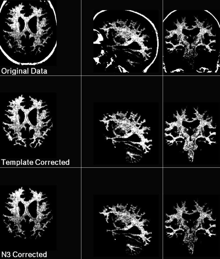
Fig. 5.

Example slices (transaxial left, sagittal middle, coronal right) through data for subject 2. Top row shows original MRI displayed with a narrow intensity range to illustrate local inhomogeneity effects, middle row shows the correction map estimated using the template-based approach and the lower row shows the N3 intensity correction map (correction maps are masked to the region used to estimate the N3 correction). Example regions of relative signal loss and gain are highlighted in the images. Note the improved localized correction (dark indicating reduction in intensity, light indicating enhancement in intensity) using the template map in these regions compared to those of the N3 method with default parameters.

Fig. 6.

Example slices (transaxial left, sagittal middle, coronal right) through data for subject 7. The MRI data is displayed with a narrow intensity range, normalised to have an equivalent range in each scan, in order to illustrate the difference in bias correction methods. Top row shows the original data, middle row shows the template corrected estimate and lower row shows the N3 corrected estimate. Note N3 has recovered loss of intensity in the cerebellum (sagittal slices), but does not recover as much signal loss as the template correction estimate in the parietal lobe (transaxial slices) or brain stem (coronal slices).

2) Coefficient of Variation

The RMS error gives a global measure of how well each automated estimate matches the manual estimate. However, it cannot tell us that we have correctly removed any residual inhomogeneity, since there remains the possibility that we have simply enforced the pattern of inhomogeneity present in our template onto each subject scan. We have, therefore, examined a second measure to give us more insight into how the methods are behaving: The coefficient of variation of intensity within a uniform region of tissue, given by the standard deviation of the intensities divided by their mean value. We derived this directly from the manually selected conservative white matter mask used to estimate the manual bias estimate in each subject. This region covers a large extent of the brain volume and, therefore, provides a sensitive measure of inhomogeneity. Plots of these coefficients of variation, for varying levels of bias estimation filter width, are shown in Fig. 7 for each test subject scan. These plots reveal that the underlying intensity variation, which should be minimized if inhomogeneity is actually being removed, does consistently decrease as the filter width is reduced. More importantly, these show that the level of white matter intensity variation falls below that in the N3 corrected estimate, at template bias filter widths of between 20 and 50 mm FWHM. The shape of each contour is roughly similar, with the scan with the highest level of inhomogeneity, signal loss and noise (subject 3) being much less sharply curved. The trend toward reduced variation breaks down in most subjects at very narrow filter widths of between 5 and 15 mm, presumably as the misregistration of tissues at the border of white matter dominate. It is interesting to note that the manual bias field estimate, using a spline fit to the masked values, has consistently reduced variation to a level between 0.059 and 0.08 across all scans. The N3 estimate generally reduces the variation to a level roughly half way between the starting variation and the manual estimate.

Fig. 7.

Coefficient of variation (Standard deviation/Mean) of intensity values within the white matter mask used for manual intensity correction for the template-based estimate as the bias estimate filter width is varied. The deformation model used in spatial normalisation for each estimate was that provided by iteration to the the finest resolution 1.8-mm B-Spline lattice. For comparison the levels of the coefficient of variation for the uncorrected data, the N3 corrected data and the spline fitted (manual) corrected data are shown.

One plausible reason for the limited removal of intensity variation using the N3 method is the default coarse model used by the N3 correction scheme. Although configured for typical physical models of the expected RF distortion effects, which are generally slowly varying, the method does not take into account the amount of tissue signal available at the cortex from which to estimate the bias field, which may be limited in atrophied brains. This may be a particular problem at the atrophied cortical surface where there are only sparse regions of tissue exhibiting signal that will usefully support the bias estimate. We, therefore, selected one of the subjects on which to carryout further N3 experiments (subject 7, shown in Fig. 6. The parameter for N3 controlling the smoothness of the bias estimated is by default set to a value of 200 mm. This controls the distance over which the distortion values are unrelated, corresponding to the support (rather than knot spacing) provided by the B-Spline model. We took the corrected estimate using this default setting and re-applied the N3 correction using parameter settings down to finer spatial models, and evaluated the resulting coefficient of variation in the white matter region for each setting. The coefficient of variation for refined estimates from a starting coefficient of variation of 0.0733, using N3 settings of 100, 50, and 25 mm were 0.0730, 0.0721, and 0.0722 respectively. Comparing these to the levels shown in Fig. 7, reveals some improvement, but the small increase in the coefficient of variation between 50 and 25 mm indicates that the results may not be usable at finer bias models. Overall, none of the estimates reduced the coefficient of variation to a comparable level to those of the template estimate (0.0692). In addition, the finer N3 model required a significantly greater computational time to converge (greater than 1.5 h).

C. The Influence of Spatial Transformation Model

In the previous experiments we have evaluated the bias field using the complete four-level deformation estimate, when mapping between template and subject MRI. For all scans we experimentally found that the finest deformation lattice provided quantifiably the greatest reduction in residual intensity variation, when using a estimation filter width at or around the optimum identified in the previous experiments. To illustrate this we include two typical plots of the the RMS error with respect to the manual bias field estimate evaluated for the four deformation levels of the nonrigid registration procedure (1.8, 3.6, 7.2, and 14.4 mm). These plots (again after rescaling to remove differences in the global mean intensity value after correction) are shown in Fig. 8. These both show that the finest deformation levels are required for optimum performance. As discussed in the previous sections, although the scale of the global RMS errors appear small, they correspond to visually detectable improvements in tissue intensity maps. The relative processing time for each level is in proportion to the number of deformation parameters being estimated which is the cube of the parameter spacing, with the total time taking between 2 and 3 h on a 1.7-GHz Pentium system. Although this numerical reduction in error from coarse to fine deformation model appears small, the improvement brings the residuals below the level of the N3 estimate in both cases. As we have seen in Fig. 5, such small distortions are still visually detectable and, therefore, pose a confound to accurate tissue classification.

Fig. 8.

The convergence of the template-based estimate toward the manual bias field correction estimate as the resolution of the deformation model is increased (Illustrated by the RMS intensity difference between the template-based and manual correction) for two of the test images.

D. Choice Width for Automated Correction of Dementia Data

The plots of RMS error and white matter intensity coefficient of variation reveal that there is, in practice, a range of optimum values for the bias filter width between different scans, as summarized for our data in Table I. This is not altogether unexpected since the optimum matched filter for the bias field will always be a function of the underlying shape of the bias field. In general, the estimation filter must separate tissue template misregistration error, in the form of high spatial frequencies, from the slower varying bias field. For a scan with a given amount of template misregistration, a sharper localized distortion, perhaps at the edge of the brain, will require a narrower filter for optimal estimation, whereas a scan with a more smoothly varying bias field can be captured by a correspondingly wider filter width which allows a greater proportion of the misregistration error to be removed. It is important to note here that we use the overall RMS intensity error over the whole brain as a guide, rather than the coefficient of variation derived from the manual white matter mask. Although most of these plots show a favorable reduction in inhomogeneity down to a very narrow estimation filter width, they do not give a true measure of correction including all anatomical boundaries in the image data. We, therefore, focus on the global RMS error relative to the Spline fitted correction estimate. In order to setup an automated correction scheme, we need to choose a compromise filter size which we can use to apply to new data. Although we have a limited number of subjects available with manual segmentations for validation, we have taken care to ensure that this data has a large range of both distortion levels and anatomies. Examination of a summary of results shown in Table I reveals that a 20-mm filter width, although not optimum for each individual, provides a good compromise, close to optimal for all scans. In addition, results using this setting for each subject show clear improvements over the N3 method.

TABLE I.

RMS Intensity Errors Relative to the Manual Segmentation Derived Bias Field Estimates, Evaluated Over the N3 Correction Mask Volume. The Minimum RMS Error, Together With the Filter Width at Which it Occurred Is Shown for Each Subject. In Addition, the RMS Error at the Filter Width of 20 mm Is Shown, for Use as a Possible Fixed Parameter Setting for Automated Processing of This Data

Subject	Opt. Width (mm)	Min Error (R.M.S.)	Error at 20mm (R.M.S.)	N3 Error (R.M.S.)
1	17 (±1)	1.53	1.54	1.73
2	35 (±5)	1.35	1.63	1.93
3	20 (±1)	5.69	5.70	6.31
4	25 (±1)	1.57	1.60	1.97
5	22 (±1)	1.35	1.35	1.80
6	15 (±1)	1.96	2.02	2.05
7	23 (±1)	1.15	1.17	1.78
8	20 (±1)	1.20	1.20	1.74
9	20 (±1)	1.38	1.38	1.84

IV. Discussion

Current retrospective methods of brain MRI bias field correction generally ignore the occurrence and spatial distribution of the range of intermediate tissue-intensity types that occur in normal T1-weighted brain MRI scans. Subtle normal differences for example, in the intensity of cortical and subcortical gray matter, pose a direct confound to the accurate estimation of nonuniformity, since global correction techniques may force these different tissue types to incorrectly exhibit the same intensity value. In this paper, we have, therefore, explored an alternative registration driven, template-based approach to correcting subtle sensitivity variations. Rather than imposing constraints purely on the global intensity distribution of an MRI scan in order to define a correction criterion, we have exploited the ability of an entropy driven spatial normalisation algorithm to map intensity distorted MRI data to a tissue reference template, in order to estimate the spatial variation in tissue intensity.

A. Validation

Validation is an important issue when claiming the correction of very subtle intensity variations. A recent paper by Arnold et al. [1] compared six different methodologies using a range of approaches including the use of repeat acquisitions. In our work, we have focused on the correction of data specific to our particular application in studying dementia and aging, and have chosen to develop our template-based approach using the N3 method of Sled [35], one of the two best methods identified by Arnold, for comparison. One of the key factors for our approach is the need to accurately account for anatomical differences in the spatial distribution of tissues between subject and template anatomies. This is particularly challenging in our application in the study of aging and degenerative disease, where spatially varying patterns of tissue loss can significantly modify brain shape. We have shown that using an hierarchical deformation refined down to a parameter lattice spacing of 1.8 mm, combined with a 20-mm estimation filter, we can recover both subtle and more extreme levels of inhomogeneity over a range of subject anatomies.

The comparative results provided by the N3 method were created by using the default parameters, with care taken to use a brain masked volume to exclude the influence of extra-cranial tissues. The N3 method did consistently remove intensity variation from our data, confirming the results of Arnold [1], however, our approach appeared to be able to remove additional variation. We believe better results may be provided by the N3 method by careful calibration of the parameters for our data, by allowing a finer bias field parameterization. However, experiments indicated that this produced only limited improvements that did not match those of the template method.

B. Methodological Issues

In this paper, we have focused on a direct approach to bias field estimation, relying entirely on the registration step to provide a map of intensity distortion at each voxel. The closest work to this is perhaps that of Ashburner et al. [2], and also Warfield etal. [44] who employed a coarse atlas matching process to provide priors to a combined intensity correction and tissue segmentation step. However, these approaches only form a weak statistical link between the bias field and intensity correction step available from a coarse spatial normalisation. In our approach, we make use of a high resolution local transformation to a template allowing the direct estimation of the residual intensity ratio between template and subject scans. The main drawback of our approach, for pure intensity correction of single studies, is the computational expense of registration between the template and the scan to be corrected, with registration taking between 2 and 3 h on a 1.7-GHz Pentium system. However, we believe the additional accuracy provided by the approach makes the technique extremely valuable in larger scale structural imaging studies of neurodegeneration, where many hundreds of studies are acquired over 3 to five years, and the sensitive detection of subtle local changes in tissue volume are the focus of the research. In the context of studies where spatial normalisation to a template is already being carried out, it provides a direct, highly accurate and fully automated method of distortion correction with little additional processing required.

We were initially concerned by the apparent need for a relatively fine-scale model of distortion for optimum correction. This seems to contradict some of the basic physics models of pure RF field effects [34], [33]. However, we feel, based on our extensive validation, combined with visual inspection of some of the distortion in the MRI data, that the subtle distortion effects are real and not anatomical. It may be that the change in shape of the brain tissue (larger ventricles and expanded sulcal CSF spaces) in aging and dementia modifies the RF effects to produce different bias fields in these anatomies. Alternatively, these structural changes may make the process of estimating a coarse bias field, for example at the cortical surface, more difficult, since the underlying tissue signal to support the bias estimate is sparsely distributed. By using a more localized model, we may allow more sensitivity to signal loss at the edges of the brain, counteracting this lack of support.

A plausible direction to further develop our approach is to build in a more robust bias filter estimation step that is less sensitive to local outliers where voxels are mis-aligned or lesions are present, which could replace the direct filter estimates of (7) and (8). A second, but much more computationally expensive modification would be to iteratively refine the registration and bias estimates together, to handle cases of large-scale intensity distortion. In our test data, in only one scan, subject 3, containing an extreme distortion example, did an additional re-registration provide further improvement in the residual errors. This is a rare case and in over 300 other scans in our study this level of distortion has not been observed. We, therefore, infer that for typical dementia data acquired in our studies, a further registration and bias estimation step will generally not be required.

One major assumption made in this paper is that the relative contrast between different tissue types in the brain is consistent between subjects. This is most obviously invalid when considering the effects of white matter disease that occurs in aging subjects. Unlike the less common problem of correcting inhomogeneity in the presence of multiple sclerosis lesions, which has been examined by Van Leemput [21] et al., more common white matter signal hyper intensities can have significant contrast in T1-weighted MRI and occupy a large fraction (> 50%) of the white matter volume in older subjects. The subjects studied in this paper did not include extreme examples of such cases. However, the nature of such white matter effects, often consisting of large, diffuse regions of reduced contrast white matter in T1-weighted MRI, would have directly contaminated the bias field estimates. Such phenomena are equally problematical for all retrospective inhomogeneity correction methods. Taking the general approach of using an atlas template for intensity distortion estimation provides us with the opportunity to introduce spatial priors into the correction step, which are unavailable to intensity-only model-based approaches. The direction of our new work will examine such approaches to dealing with the separation of diffuse disease induced effects, from scanner induced inhomogeneity.

C. Conclusion

Accurate and sensitive detection of tissue volume differences from high resolution MRI studies is dependent on the correct assignment of tissue classification based on the observed MRI intensity across a population being studied. In particular, applications requiring the localized detection and mapping of change in tissue volume will be the most sensitive to regional variations in tissue intensity. An example of such applications is serial deformation tensor morphometry [12]. Here, small-scale tissue volume changes are captured over time within each subject using a highly localized volume registration scheme. A group pattern of common volume change can be created [37], by transforming each map to a common template. When analyzing these maps [36] acquired from different subjects, it is important to separate changes observed in different tissues types (for example contractions in white or gray matter from expansions in CSF), to ensure optimum separation of tissues. Accurate correction of intensity bias in the image data of each subject is then critical in assessing the anatomical location of volume change over time.

Large-scale population-based studies are increasingly important in the study of neurodegenerative conditions. In such studies it is common to maintain the same acquisition type and scanner throughout the entire study. It is in such studies where we feel this template-based approach can be most valuable in helping to extract accurate measures of tissue volume and volume change, by making use of a template optimized for the contrast properties of a particular study. Overall, the experimental results we have so far indicate a promising increase in the sensitivity of bias field detection using the template-based approach. We are currently further refining the technique using improved reference templates and extending the validation of the method to a larger set of data with different age ranges and disease conditions.

References

- 1.Arnold JB, Liow JS, Schaper KA, Stern JJ, Sled JG, Shattuck DW, Worth AJ, Cohen MS, Leahy RM, Mazziotta JC, Rottenberg DA. Qualitative and quantitative evaluation of six algorithms for correcting intensity nonuniformity effects. NeuroImage. 2001;13:931–943. doi: 10.1006/nimg.2001.0756. [DOI] [PubMed] [Google Scholar]
- 2.Ashburner J, Friston KJ. Voxel-based morphometry—The methods. NeuroImage. 2000;11:805–821. doi: 10.1006/nimg.2000.0582. [DOI] [PubMed] [Google Scholar]
- 3.Axel L, Costantini J, Listerud J. Intensity correction in surface-coil MR imaging. Amer. J. Radiol. 1987;148:418–420. doi: 10.2214/ajr.148.2.418. [DOI] [PubMed] [Google Scholar]
- 4.Brinkmann BH, Manduca A, Robb RA. Optimized homomorphic unsharp masking for MR greyscale correction. IEEE Trans. Med. Imag. 1998 Apr.17:161–171. doi: 10.1109/42.700729. [DOI] [PubMed] [Google Scholar]
- 5.Christensen GE, Rabbitt RD, Miller MI. Deformable templates using large deformation kinematics. IEEE Trans. Image Processing. 1996 May;:1435–1447. doi: 10.1109/83.536892. [DOI] [PubMed] [Google Scholar]
- 6.Collins DL, Evans AC, Holmes C, Peters TM. Automatic 3D segmentation of neuro-anatomical structures from MRI. In: Bizais Y, Barillot C, Di Paola R, editors. Proceedings of Information Processing in Medical Imaging. Kluwer Academic; Brest, France: 1995. pp. 139–152. [Google Scholar]
- 7.Collins DL, Zijdenbos AP, Sled JG, Kabani NJ, Holmes CJ, Evans AC. Design and construction of a realistic digital brain phantom. IEEE Trans. Med. Imag. 1998 June;17:463–468. doi: 10.1109/42.712135. [DOI] [PubMed] [Google Scholar]
- 8.Studholme C, Novotny E, Zubal IG, Duncan JS. Estimating tissue deformation between functional images induced by intracranial electrode implantation using anatomical MRI. NeuroImage. 2001;13:561–576. doi: 10.1006/nimg.2000.0692. [DOI] [PubMed] [Google Scholar]
- 9.Dale AM, Fischl B, Sereno MI. Cortical suface based analysis—I: Segmentation and surface reconstruction. NeuroImage. 1999;9:179–194. doi: 10.1006/nimg.1998.0395. [DOI] [PubMed] [Google Scholar]
- 10.Dawant BM, Zijdenbos AP, Mangolin RA. Correction of intensity variations in MR images for computer-aided tissue classification. IEEE Trans. Med. Imag. 1993 Dec.12:770–781. doi: 10.1109/42.251128. [DOI] [PubMed] [Google Scholar]
- 11.DeCarli C, Murphy DGM, Teichberg D, Campblell G, Sobering GS. Local histogram correction of MRI spatially dependent image pixel intensity nonuniformity. J. Magn. Reson. Imag. 1996;6:519–528. doi: 10.1002/jmri.1880060316. [DOI] [PubMed] [Google Scholar]
- 12.Freeborough PA, Fox NC. Modeling brain deformations in Alzheimer's disease by fluid registration of serial 3D MR images. J. Comput. Assist. Tomogr. 1998;22(5):838–843. doi: 10.1097/00004728-199809000-00031. [DOI] [PubMed] [Google Scholar]
- 13.Friston KJ, Ashburner J, Frith CD, Poline JB, Heather JD, Frackowiak RSJ. Spatial registration and normalisation of images. Human Brain Mapping. 1995;2:165–189. [Google Scholar]
- 14.Guillemaud R, Brady M. Estimating the bias field of MR images. IEEE Trans. Med. Imag. 1997 July;16:238–251. doi: 10.1109/42.585758. [DOI] [PubMed] [Google Scholar]
- 15.Höhne KH, Hanson WH. Interactive 3D segmentation of MRI and CT volumes. J. Comput. Assist. Tomogr. 1992;16(2):285–294. doi: 10.1097/00004728-199203000-00019. [DOI] [PubMed] [Google Scholar]
- 16.Jernigan TL, Archibald SL, Fennema-Notestine C, Gamst AC, Stout JC, Bonner J, Hesselink JR. Effects of age on tissues and regions of the cerebrum and cerebellum. Neurobiol. Aging. 2001;22(4):581–591. doi: 10.1016/s0197-4580(01)00217-2. [DOI] [PubMed] [Google Scholar]
- 17.Johnson B, Atkins MS, Mackiewich B, Anderson M. Segmentation of multiple sclerosis lesions in intensity corrected multispectral MRI. IEEE Trans. Med. Imag. 1996 Apr.15:154–169. doi: 10.1109/42.491417. [DOI] [PubMed] [Google Scholar]
- 18.Kochunov PV, Lancaster JL, Fox PT. High speed spatial normalisation using an octree method. NeuroImage. 1999;10:724–737. doi: 10.1006/nimg.1999.0509. [DOI] [PubMed] [Google Scholar]
- 19.Lee S, Wolberg G, Chwa KY, Shin SY. Image metamorphosis with scattered feature constraints. IEEE Trans. Visual. Comput. Graphics. 1996 Dec.2:337–354. [Google Scholar]
- 20.Lee SK, Vannier MW. Post acquisition correction of MR inhomogeneities. Magn. Reson. Med. 1996;36:275–286. doi: 10.1002/mrm.1910360215. [DOI] [PubMed] [Google Scholar]
- 21.Van Leemput K, Maes F, Vandermeulen D, Colchester A, Suetens P. Automated segmentation of multiple sclerosis lesions by model outlier detection. IEEE Trans. Med. Imag. 2001 Aug.20:667–688. doi: 10.1109/42.938237. [DOI] [PubMed] [Google Scholar]
- 22.Van Leemput K, Maes F, Vandermeulen D, Suetens P. Automated model-based tissue classification of MR images of the brain. IEEE Trans. Med. Imag. 1999 Oct.18:897–908. doi: 10.1109/42.811270. [DOI] [PubMed] [Google Scholar]
- 23.Likar B, Viergever M, Pernus F. Retrospective correction of MR intensity inhomogeneity by information minimzation. In: Delp SL, DiGiola AM, Jaramaz B, editors. Proc. MICCAI. Pittsburgh, PA: 2000. pp. 375–384. [DOI] [PubMed] [Google Scholar]
- 24.Maes F, Collignon A, Vandermeulen D, Marchal G, Suetens P. Multimodality image registration by maximization of mutual information. IEEE Trans. Med. Imag. 1997 Apr.16:187–198. doi: 10.1109/42.563664. [DOI] [PubMed] [Google Scholar]
- 25.Meyer CR, Bland PH, Pipe J. Retrospective correction of intensity inhomogeneities in MRI. IEEE Trans. Med. Imag. 1995 Feb.14:36–41. doi: 10.1109/42.370400. [DOI] [PubMed] [Google Scholar]
- 26.Nocera L, Gee JC. Robust partial-volume tissue classification of cerebral MRI scans. Proc. SPIE (Geometric Methods in Computer Vision II) 1997;3034:312–322. [Google Scholar]
- 27.Pham D, Prince J. Adaptive fuzzy segmentation of magnetic resonance images. IEEE Trans. Med. Imag. 1999 Sept.18:737–752. doi: 10.1109/42.802752. [DOI] [PubMed] [Google Scholar]
- 28.Rajapakse JC, Kruggel F. Segmentation of MR images with intensity inhomogeneities. Image Vis. Computing. 1998;16:165–180. [Google Scholar]
- 29.Ruckert D, Hayes C, Studholme C, Leach M, Hawkes DJ. Nonrigid registration of breast MR images using mutual information. In: Wells WM, Colchester A, Delp S, editors. Proc. MICCAI. Cambridge, MA: 1998. pp. 1144–1152. [Google Scholar]
- 30.Ruckert D, Sonoda LI, Hayes C, Leach MO, Hawkes DJ. Nonrigid registration using free-form deformations: Application to breast MR images. IEEE Trans. Med. Imag. 1999 Aug.18:712–721. doi: 10.1109/42.796284. [DOI] [PubMed] [Google Scholar]
- 31.Schormann T, Henn S, Bürgel U, Engler K, Zilles K. A new technique for 3-D nonlinear deformation: Application to studies of the variability of brain structures. NeuroImage. 1997:S418. [Google Scholar]
- 32.Shattuck DW, Sandor-Leahy SR, Schaper KA, Rottenberg DA, Leahy RM. Magnetic resonance image tissue classification using a partial volume model. NeuroImage. 2001;13:856–876. doi: 10.1006/nimg.2000.0730. [DOI] [PubMed] [Google Scholar]
- 33.Sled JG, Pike B. Standing-wave and RF penetration artifacts caused by elliptic geometry: An electrodynamic analysis of MRI. IEEE Trans. Med. Imag. 1998 Aug.17:653–662. doi: 10.1109/42.730409. [DOI] [PubMed] [Google Scholar]
- 34.Sled JG, Pike GB. Understanding intensity non-uniformity in MRI. Proc. MICCAI. 1998:614–622. [Google Scholar]
- 35.Sled JG, Zijdenbos AP, Evans AC. A nonparametric method for automatic correction of intensity nonuniformity in MRI data. IEEE Trans. Med. Imag. 1998 Feb.17:87–97. doi: 10.1109/42.668698. [DOI] [PubMed] [Google Scholar]
- 36.Studholme C, Cardenas V, Maudsley A, Weiner M. An intensity consistent approach to the cross sectional analysis of deformation tensor derived maps of brain shape; Proc. 5th Int. Conf. MICCAI; 2002. pp. 492–499. [DOI] [PubMed] [Google Scholar]
- 37.Studholme C, Cardenas V, Weiner M. presented at the ISMRM. Glasgow, Scotland: 2001. Building whole brain maps of atrophy from multi-subject longitudinal studies using free form deformations. [Google Scholar]
- 38.Studholme C, Cardenas V, Weiner M. Multi scale image and multi scale deformation of brain anatomy for building average brain atlases. Proc. SPIE (Medical Imaging) 2001;4322-60:557–568. [Google Scholar]
- 39.Studholme C, Constable RT, Duncan JS. Accurate alignment of functional EPI data to anatomical MRI using a physics-based distortion model. IEEE Trans. Med. Imag. 2000 Nov.19:1115–1127. doi: 10.1109/42.896788. [DOI] [PubMed] [Google Scholar]
- 40.Studholme C, Hill DLG, Hawkes DJ. An overlap invariant entropy measure of 3D medical image alignment. Pattern Recogn. 1999;32(1):71–86. [Google Scholar]
- 41.Styner M, Brechbhler C, Szkely G, Gerig G. Parametric estimate of intensity inhomogeneities applied to MRI. IEEE Trans. Med. Imag. 2000 Mar.19:153–165. doi: 10.1109/42.845174. [DOI] [PubMed] [Google Scholar]
- 42.Thirion J-P. Image matching as a diffusion process: An analogy with maxwell's demons. Med. Image Anal. 1998;2(3):243–260. doi: 10.1016/s1361-8415(98)80022-4. [DOI] [PubMed] [Google Scholar]
- 43.Wang L, Lai HM, Barker GJ, Miller DH, Tofts PS. Corrections for variations in MRI scanner sensitivity in brain studies with histogram matching. Magn. Reson. Med. 1998;39:322–327. doi: 10.1002/mrm.1910390222. [DOI] [PubMed] [Google Scholar]
- 44.Warfield SK, Kaus M, Jolesz FA, Kikinis R. Adaptive, template moderated, spatially varying statistical classification. NeuroImage. 2000;4:43–55. doi: 10.1016/s1361-8415(00)00003-7. [DOI] [PubMed] [Google Scholar]
- 45.Wells W, Grimson W, Kikinis R, Jolesz F. Statistical intensity correction and segmentation of MRI data. Proc. SPIE (Visualisation Biomedical Computing) 1994;2359:13–24. [Google Scholar]
- 46.Wells WM, Grimson WEL, Kikinis R, Jolesz FA. Adaptive segmentaion of MRI data. IEEE Trans. Med. Imag. 1996 Aug.15:429–442. doi: 10.1109/42.511747. [DOI] [PubMed] [Google Scholar]
- 47.Wells WM, Viola P, Atsumi H, Nakajima S, Kikinis R. Multi-modal volume registration by maximisation of mutual information. Med. Image Anal. 1996;1(1):35–51. doi: 10.1016/s1361-8415(01)80004-9. [DOI] [PubMed] [Google Scholar]
- 48.Woods RP, Grafton ST, Watson JD, Sicotte NL, Mazziotta JC. Automated image registration II: Intersubject validation of linear and non-linear models. J. Comput. Assist. Tomogr. 1998;22:153–165. doi: 10.1097/00004728-199801000-00028. [DOI] [PubMed] [Google Scholar]
- 49.Yan MXH, Karp JS. An adpative baysian approach to three dimensional MR brain segmentation. In: Bizais Y, Barillot C, Di Paola R, editors. Proceedings of Information Processing in Medical Imaging. Brest, France: 1995. pp. 201–213. [Google Scholar]