

Abstract
Objective
This study examined the effects of leaving home and going to college on changes in the frequency of alcohol use, heavy episodic drinking, and marijuana use shortly after leaving high school. We also examined how protective factors in late adolescence predict post-high school substance use and moderate the effects of leaving home and going to college.
Method
Data came from subjects (N = 319; 53% male) interviewed at the end of 12th grade and again approximately 6 months later, as part of the Raising Healthy Children project.
Results
Leaving home and going to college were significantly related to increases in the frequency of alcohol use and heavy episodic drinking from high school to emerging adulthood but not to changes in marijuana use. Having fewer friends who used each substance protected against increases in the frequency of alcohol use, heavy episodic drinking, and marijuana use. Higher religiosity protected against increases in alcohol-and marijuana-use frequency. Higher parental monitoring protected against increases in heavy episodic drinking and moderated the effect of going to college on marijuana use. Lower sensation seeking lessened the effect of going to college on increases in alcohol use and heavy episodic drinking.
Conclusions
To prevent increases in substance use in emerging adulthood, interventions should concentrate on strengthening prosocial involvement and parental monitoring during high school. In addition, youths with high sensation seeking might be targeted for added intervention.
The transition out of high school is one of the most critical passages in life because of pronounced changes in social environment and role responsibilities (Newcomb and Bentler, 1987). Increases in substance use are evident during this transitional period (Arnett, 2005; Bachman et al., 1997). Arnett (2005) has argued that these increases occur because this stage of the life cycle, which he has termed “emerging adulthood,” provides more freedom and less social control than the high school years. Several researchers have attributed these increases, especially in heavy drinking, specifically to the college experience (Goldman et al., 2002). White and colleagues (2005), however, found that increases in cigarette smoking, marijuana use, alcohol intoxication, and alcohol problems occurred as individuals left high school, regardless of whether they attended college (see also Bingham et al., 2005). Bachman and colleagues (1997) suggested that it was living situation (with friends and roommates vs parents or spouses) that accounted for increased substance use during this transitional period, rather than the college experience per se. As these increases are not universal, however, it is important to identify the individual and environmental factors that influence changes in substance use from late adolescence into emerging adulthood. The purpose of this article is twofold: (1) to examine the effects of leaving home and going away to college on changes in substance use approximately 6 months after leaving high school, and (2) to examine how protective factors measured in late adolescence predict change in substance use and moderate the effects of leaving home and going to college.
Transitions during emerging adulthood
Emerging adulthood is defined as the stage of the life cycle that begins following high school and ends with the adoption of adult roles (e.g., marriage, parenthood, and career); it spans roughly the ages 18–25 years (Arnett, 2000). This stage represents a time when most youths initiate new roles; many develop new friendship networks, and many separate from their families (Arnett, 2005; Schulenberg and Maggs, 2002). Arnett (2005) has argued that decreasing social control and increasing instability and stress contribute to increases in alcohol and drug use during emerging adulthood. In addition, the weakening of parental monitoring and increased importance of peer relationships can lead to increased substance use (Borsari and Carey, 2001).
Several prospective studies of college students have demonstrated that as they moved out of their parents’ homes into dormitories or off-campus living situations, students’ heavy drinking increased (e.g., Baer et al., 1995; Harford and Muthén, 2001). In general, these studies have focused on students at 4-year colleges. Studies of students at 2-year colleges indicate that they drink less than those at 4-year colleges (Presley et al., 2002; Sheffield et al., 2005). This research, however, has not accounted for differential living arrangements (i.e., more 2-year than 4-year college students remain living at home); neither has it examined changes in use from high school to college. Although increases in substance use have been most often identified for those young adults who go to college and move away from their parents, noncollege-bound youths who move out of their parents’ homes experience many of these changes as well (Dawson et al., 2004; White et al., 2005). Bachman and colleagues (1997) found that college students (2- and 4-year combined), as compared with their noncollege peers, reported lower rates of heavy drinking while in high school; however, their use increased when they entered college, resulting in higher levels than those of their noncollege peers. College students also increased their marijuana use from high school to college, but they did not surpass their noncollege peers, who reported a higher prevalence both during high school and in emerging adulthood. Increases in alcohol and marijuana use for college students were attributed to living in dormitories or similar housing shared with other young adults (see also Crowley, 1991).
Using national data, Gfroerer and colleagues (1997) found that educational status and living situation were significant predictors of cigarette, cocaine, marijuana, and alcohol use, as well as heavy drinking. Rates of past-month marijuana use were highest among high school dropouts who lived with their parents and college students not living with parents; current and heavy drinking were highest among college students who did not live with their parents. College students who lived with their parents reported the lowest rates of marijuana use and heavy drinking. These studies highlight the importance of considering both changes in living situation (i.e., moving away from home) and school status (i.e., going to college) as potential risk factors for increases in substance use during the transition out of high school into emerging adulthood. Nevertheless, not all emerging adults increase their substance use as they move away from home or enter college. Therefore, it is important to delineate those protective factors in high school that moderate the transition to higher levels of substance use after high school.
Potential high school protective factors
Protective factors have been defined differently across studies (see Stouthamer-Loeber et al., 2002, for a detailed discussion). Some researchers have referred to variables as if they are either uniquely protective or uniquely related to risk (e.g., Rae-Grant et al., 1989). Others consider risk and protection as a continuum, with scores on one end of a variable indicating risk and scores on the other end indicating protection (Stouthamer-Loeber et al., 2004). Still others have conceptualized protective factors as processes that play a special role in the presence of risk (Hawkins et al., 1992; Rutter, 1990), reflecting interaction effects; in this case, the effect of a protective factor is greater when risk is high than when risk is low. We follow the latter two approaches and examine main effects, as well as whether protective factors moderate the effects of two potential risk factors: going to college and moving away from home.
Our choice of protective factors was guided by the Social Development Model (SDM; Catalano and Hawkins, 1996, 2002). The SDM incorporates the most strongly supported propositions of social control, social learning, and differential association theories into a developmental framework that describes the onset, progression, and cessation of prosocial and antisocial behaviors (Catalano and Hawkins, 1996; Catalano et al., 2005). The SDM postulates that children learn prosocial and antisocial behaviors from socializing agents in the context of family, school, peer groups, and religious and other community institutions. The development of behavior (prosocial or antisocial) is hypothesized to be a result of environmental opportunities for involvement, individual skills and capacities to be successful in their involvement, and the rewards forthcoming from involvement. A bond between the individual and the socializing unit develops when socialization experiences are consistent. When those in the socializing unit hold prosocial beliefs, the individual tends to internalize these beliefs and is more likely to engage in prosocial behavior and less likely to engage in antisocial behavior. The reverse is hypothesized to occur for those who develop bonds with individuals or groups with antisocial beliefs. In addition, external constraints (e.g., parental rules and monitoring) and individual constitutional factors (e.g., sensation seeking) are hypothesized to impact the socialization experiences (Catalano et al., 2005). The protective factors selected for the present study are high parental monitoring (Peterson et al., 1994; Schulenberg and Maggs, 2002; Wood et al., 2004), low sensation seeking (Arnett, 2005; Bates et al., 1985; Jackson et al., 2005), involvement with nonsubstance-using peers (Bates and Labouvie, 1997; Jackson et al., 2005; Wood et al., 2004), high religiosity (Jackson et al., 2005; Steinman and Zimmerman, 2004; Wallace et al., 2003), high achievement in school (Newcomb et al., 2002), and strong bonding to school (Hawkins et al., 1992). All of these measures tap critical elements of the SDM. Based on the SDM, it is expected that prosocial involvement, skills, and bonding in late adolescence will reinforce prosocial behavior, increase prosocial beliefs, and lead youth to seek out like individuals and activities that reinforce prosocial beliefs, maintaining a prosocial course of development in which substance use will be less likely (Catalano and Hawkins, 1996). Further, parental monitoring is expected to enhance these prosocial processes and those with low sensation seeking are expected to experience prosocial socialization processes as reinforcing. Thus, both internal constraints and constitutional factors measured in high school are expected to protect youths once they leave and are exposed to new environments.
Current study
This study focuses on changes in frequency of alcohol use, heavy episodic drinking, and marijuana use during the transition out of high school. We examine whether leaving home and going to either a 2- or 4-year college, as well as their interaction, are related to changes in substance use. Further, we examine whether protective factors measured prospectively in the 12th grade predict changes in substance use approximately 6 months later and moderate the effects of leaving home and going to college on subsequent substance use. To our knowledge, this is the first study to have collected substance-use data prospectively, from both college students and their noncollege peers, over a short time interval during this transitional period.
We hypothesize that (1) college attendance will be related to increases in all types of substance use, especially heavy episodic drinking; and (2) those young adults who move away from home will experience greater increases in substance use than those who stay home, regardless of whether they attend college. We also hypothesize that higher parental monitoring, fewer peers who use drugs, higher school bonding and achievement, lower sensation seeking, and higher religiosity measured in the senior year of high school will predict less frequent substance use during emerging adulthood and will reduce increases in substance use for those who go to college and move away from home.
Method
Design and sample
Data come from the Raising Healthy Children project (RHC), a multiwave longitudinal study of the development of substance use from childhood into young adulthood. The study population consisted of first- and second-grade students in 10 suburban public elementary schools in a Pacific Northwest school district. In 1993–94, 1,040 students (76% of those eligible) were recruited. These students were interviewed every spring through the 12th grade and once more, in the fall, 6 months later. The fall survey was added to capture short-term changes in substance use following high school. Approximately half (54%) of the participants had been part of a prevention project from elementary school through high school; therefore, we control for whether participants were in the intervention or control group in the analyses (for more details of the intervention and the study design, see Brown et al., 2005; Catalano et al., 2003; Haggerty et al., 1998). The present study uses only members of the older cohort (original N = 501), who were in second grade at the beginning of the study, because post-high school data are not yet available for the younger cohort. The retention rate has been quite high, with an overall response rate of 90% in the 12th grade and 86% for the fall survey. Those who dropped out were similar to those retained with respect to baseline gender, ethnicity, and low-income status (i.e., whether they received free/reduced-price school lunch in the first 2 years of the project).
The sample for the present analysis includes only those individuals who completed both the 12th-grade and fall surveys. Because we wanted prospective data on the transition out of high school and away from home, we also eliminated those youths who were not in high school and/or were not living at home at the time of the 12th-grade spring survey. Thus, during the 12th-grade survey, those who reported already being in college (n = 26), already graduating or earning a GED (n = 16), currently taking GED courses (n = 7), and having dropped out of high school (n = 40), as well as those still in high school but not living with their parents or a parental figure (n = 13), were excluded from these analyses. The final sample size for the present analyses is 319. The 102 excluded participants reported significantly (p < .001) higher rates of alcohol and marijuana use during the 12th-grade and fall assessments and significantly (p < .05) lower scores on all of the protective factors, with the exception of parental monitoring, compared with the final analysis sample.
The analysis sample was 53% male, and the average age of youth during the fall survey was 18.7 years (range: 17.9–19.9). The sample was 82% white, 8% Asian or Pacific Islander, 4% Hispanic, 3% black, and 2% Native American; 22% of participants received free or reduced-price school lunch in the first 2 years of the project.
Procedures
The RHC project was approved by the University of Washington Human Subjects Review Committee. The 12th-grade spring survey was administered one-on-one between March and May of 2004 by an interviewer who recorded student answers on a laptop using the Computer-Assisted Personal Interview (CAPI) technique. For sensitive questions (e.g., substance use), participants answered questions directly onto the computer. The interview took an average of 50 minutes to complete, and participants received a $15 cash incentive. Most youths were interviewed again during the fall (October-December) of 2004, although a small number (n = 26) were interviewed in January 2005. About half completed the survey over the Internet, and half were interviewed in person using the same CAPI technique as in high school. Participants received a $20 cash incentive for the fall survey, which averaged about 30 minutes to complete. Analyses indicate no differences in responses to substance-use questions between modes of administration (Petrie et al., 2005).
Measures
We used self-report data from both the spring of 12th grade and the following fall. Self-reports have generally been found to be reliable for assessing substance-use behaviors (Darke, 1998; Johnston et al., 2004; Needle et al., 1983).
Substance-use measures
The substance-use measures were identical in the 12th grade and fall surveys. Past-month frequencies of alcohol use, marijuana use, and heavy episodic drinking (occasions of drinking five or more drinks for men and four or more drinks for women; Wechsler et al., 2000) were assessed on an ordinal scale, ranging from 0 (never) to 6 (40 or more times). (See Table 1 for descriptive information on all study variables.) Response categories for all three substance-use measures were recoded, assigning the midpoint of each ordinal category to create an interval measure of the number of times in the past month. To reduce highly skewed distributions, we transformed frequency scores by adding a constant (1) and took the natural logarithm of the number of use episodes. The multivariate analyses use these natural logarithmic scores as the metric for our dependent variables; however, unlogged means are shown in Table 1 and Figure 1 to aid in interpretation of the findings.
Table 1.
Correlations among substance-use variables, college and living status, and protective factors (N = 319)
 |
Notes: GPA = grade point average.
All correlations are Pearson’s, with the exception of these two columns, which are Spearman correlations.
p < .05;
p < .01;
p < .001.
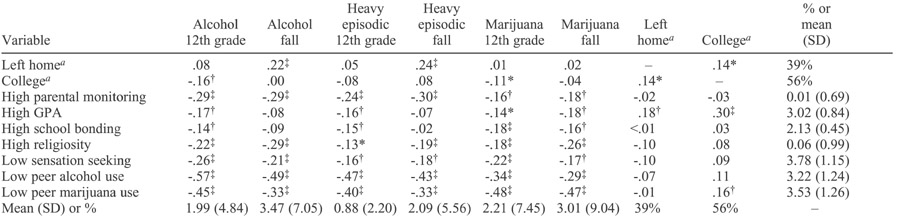
Figure 1.
College status and living status differences in the frequency of alcohol use, heavy episodic drinking, and marijuana use. Note: Unlogged means shown.
Transitions
College status was coded 1 if the youth was enrolled in a 2- or 4-year college (n = 180) and 0 if the youth was working, unemployed, or still attending high school or an alternative school (n = 139) during the fall survey. (Note that we combined 2- and 4-year college students. A large proportion of college students in the state of Washington begin at 2-year schools and then transfer to 4-year schools; combining the two also allows us to maintain larger cell sizes for the analyses. The majority of college students in our sample remained in the state of Washington, although about 20% went out of state.) Living status was coded 1 if the youth had left home and was not living with his/her parents/caretakers (n = 123) and 0 if the youth was still living with his/her parents/caretakers (n = 196) at the time of the fall survey.
Protective factors
Parental monitoring was a seven-item scale that combined four items (e.g., “When you are not home, your parents know where you are and who you are with.”) from the Parental Monitoring scale (Steinberg et al., 1994) and three items (e.g., “Do you keep a lot of secrets from your parents about what you do during your free time?”) from the Child Disclosure scale (Kerr and Stattin, 2000), as reported by the youth. These items were standardized and scores were averaged (α = .83). School achievement was a single item that asked about grades in the past year, ranging from 0 (mostly E’s or F’s) to 4 (mostly A’s). School bonding was made up of four items (α = .72) assessing whether school is fun, nice things happen at school, the youth looks forward to school, and the youth tries to do well in school (response categories ranged from 1 = “big NO” to 4 = “big YES”). Sensation seeking was measured by combining two items (r = .72) asking the number of times youths did something dangerous because they were dared and the number of times they did crazy things; response categories ranged from 1 (never) to 6 (once a week or more). Religiosity was a standardized measure, created by averaging responses to two items (r = .74) about the frequency of attending religious services and the importance of religion in one’s life. We asked about the proportion of their 10 closest friends who use alcohol and use marijuana, with a range from 1 (none) to 5 (a lot). All protective factors were recoded so that the higher score means greater protection.
Control variables
In the multivariate analyses, we controlled for gender (coded 1 for male and 0 for female). To control for Christmas break and New Year’s Eve drinking, we controlled for the month the fall survey was administered (those interviewed in January were coded 1 and those in October through December were coded 0), and we controlled for whether the youth was part of the intervention (coded 1) or control group (coded 0). We also controlled for poverty through parent’s report in the last 3 years of their household receiving any of the following: food stamps, Temporary Assistance for Needy Families (TANF), Aid to Families with Dependent Children (AFDC), welfare, or free/reduced school lunch. Any report was coded 1, and no report was coded 0.
Results
The results are presented in three sections. First, we show descriptive data on the levels of substance use by college and living status. Next, we examine the bivariate associations among substance use, college and living status, and protective factors. Last, we conduct multivariate hierarchical regression analyses to test our hypotheses.
Differences in substance use for transition groups
Figure 1 shows the group means on frequency of alcohol use, heavy episodic drinking, and marijuana use in the 12th grade and 6 months later, for four groups: (1) those living at home and not going to college (n = 96), (2) those living at home and going to college (n = 100), (3) those who moved away from home and did not go to college (n = 43), and (4) those who moved away and went to college (n = 80). One-way analyses of variance indicate that there were significant differences in alcohol-use frequency in high school among the four groups (F = 3.46, 3/315 df, p = .02). Post hoc Scheffe tests indicate that those who moved away from home but did not go to college reported significantly (p < .05) more frequent alcohol use in the 12th grade than those who stayed home and went to college. There were no significant differences among the four groups in terms of their frequency of heavy episodic drinking (F = 1.58, 3/314 df, p = .20) or marijuana use (F = 1.94, 3/315 df, p = .12) during the 12th grade. Six months later, there were significant differences among the four groups in terms of frequency of heavy episodic drinking (F = 8.02, 3/314 df, p < .001) and alcohol use (F = 8.42, 3/313 df, p < .001) but not marijuana use (F = 1.47, 3/314 df, p = .22). Post hoc tests indicate that those youths who went to college and moved away from home reported significantly (p < .05) higher frequency of alcohol use and heavy episodic drinking than those who stayed home, regardless of whether they went to college.
Correlations among substance use, college and living status, and protective factors
Table 1 shows the correlations among substance use, going to college and leaving home, and protective factors as well as the means and standard deviations for each variable. All protective factors were significantly negatively related to substance use during 12th grade. Six months later, all protective variables were still significantly negatively related to marijuana-use frequency. All protective factors, except grade point average (GPA) and school bonding, were significantly negatively related to frequency of alcohol use and heavy episodic drinking in the fall.
Living status post-high school was significantly and positively correlated with heavy episodic drinking and alcohol use in emerging adulthood but not during senior year of high school. Living status was not related to marijuana-use frequency at either assessment. Going to college was significantly negatively correlated with marijuana- and alcohol-use frequency in high school but was not correlated with marijuana- and alcohol-use frequency during emerging adulthood. College status was not significantly related to heavy episodic drinking at either assessment.
There was a small significant positive relationship between going to college and leaving home. Those youths with higher GPAs in the 12th grade were more likely to attend college and to move away from home. Those with more friends smoking marijuana in 12th grade were more likely to go to college than those with fewer friends smoking marijuana. None of the protective factors were correlated at levels to suggest multicollinearity (not shown but available from the first author on request) except friends’ alcohol and marijuana use (r = .71), which are not included in the same model.
Predicting changes in substance use from high school to emerging adulthood
Multivariate analyses examined whether college and living status predicted increases in substance use from high school to emerging adulthood and whether protective factors measured in high school moderated these increases. We used a stepwise, conditional-change regression strategy to model change over time in the frequency of substance use reported by youth. For each log-transformed dependent variable of substance use, we first entered the control variables (gender, administration month, intervention-group status, and parental poverty) and the lagged substance-use variable measured in the 12th grade. By using a lagged dependent variable strategy, we are, in essence, adjusting for initial differences in substance use to yield unbiased estimates of effects. Finkel (1995) and Menard (1991) note that the two-wave lagged effects model provides a test of “Granger causality” by controlling for prior values of the dependent variable. Coefficients for prior substance use can also be interpreted as a tendency toward continuity or conditional change in substance use during the 6-month period. In the second step, we entered college and living status. In the third step, we entered the 12th-grade protective factors. Last, we separately tested the interactions of each protective factor with living status and college status, as well as the interaction between living and college status using centered interaction terms.
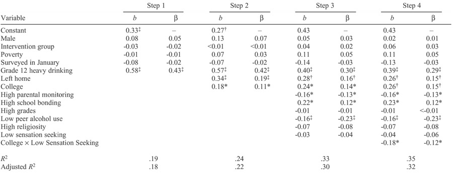
The regression results for changes in alcohol use are shown in Table 2. Step 1 shows that being male and using alcohol more frequently in the 12th grade significantly predicted higher frequency of drinking 6 months later. As shown in Step 2, there were significant main effects of going to college (b = 0.19, p < .05) and leaving home (b = 0.34, p < .001). The effect of leaving home was stronger than the effect of going to college, as indicated by the standardized coefficients, as well as an F test for unique variance explained (not shown). Adding the 12th-grade protective factors (Step 3) did not reduce the strong effects of college and living status; however, significant main effects were noted for two protective factors. Having fewer friends who drank (b = −0.13, p < .01) and higher religiosity (b = −0.11, p < .05) in the 12th grade were uniquely related to less increase in the frequency of drinking alcohol 6 months later. Only two significant interactions were significant in Step 4. The hypothesized interaction between college and living status (b = 0.47, p < .05) was significant and significantly increased the amount of variance explained compared with Step 3 (F = 9.28, 1/290 df, p < .01).
Table 2.
Alcohol frequency regression results (n = 300)
 |
Notes: Outcome variable and lagged-dependent variables are natural log transformed. Interaction terms are centered. Only significant interactions are shown in Step 4.
p < .05;
p < .01;
p < .001.
Using the technique recommended by Aiken and West (1991), we probed this interaction (see Figure 2). We found that, as indicated by the analysis of variance results above, young adults who moved away from home and attended college were the group that reported the highest frequency of alcohol use in emerging adulthood, after controlling for demographic factors, their frequency of alcohol use in high school, and the protective factors. Sensation seeking moderated the relationship between college status and alcohol use (b = −0.19, p < .05) and the addition of this interaction significantly increased the amount of variance explained in Step 3 (F = 6.48, 1/283 df, p < .05). Low sensation seekers who attended college reported a significantly lower frequency of alcohol use in emerging adulthood than high sensation seekers who attended college, whereas there was no association between sensation seeking and frequency of alcohol use for noncollege youth (see Figure 3).
Figure 2.
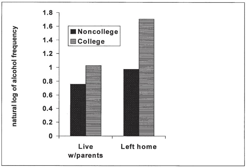
Probe of the interaction between living status and college status for changes in alcohol frequency from 12th grade to the following fall
Figure 3.

Probe of the interaction between college status and sensation seeking for changes in alcohol frequency from 12th grade to the following fall
The regression analyses predicting changes in frequency of heavy episodic drinking are shown in Table 3. In Step 1, only the lagged 12th-grade heavy episodic drinking variable significantly predicted frequency of heavy drinking 6 months later, and it remained significant in all steps. As shown in Step 2, not living at home with parents (b = 0.34, p < .001) and attending college (b = 0.18, p < .05) were both uniquely associated with greater relative increases in the frequency of heavy episodic drinking during this period. Living status was a stronger predictor than college status, as indicated by the magnitude of its standardized coefficient and an F test for unique variance (not shown). Adding the 12th-grade protective factors in Step 3 did not reduce the strong effects of college and living status; in addition, significant main effects were noted for three protective factors. Having fewer friends who drank (b = −0.16, p < .001) and higher levels of parental monitoring (b = −0.16, p < .05) in the 12th grade significantly reduced increases in the frequency of heavy episodic drinking 6 months later. It was surprising to note that higher school bonding (b = 0.22, p < .05) was positively related to greater changes in heavy episodic drinking, controlling for college and living statuses and the other protective factors. This reflects a suppressor effect of adjusting for prior heavy episodic drinking because, although heavy episodic drinking in high school was negatively associated with school bonding at the bivariate level, it was not related to school bonding in emerging adulthood at the bivariate level.
Table 3.
Heavy episodic drinking frequency regression results (n = 300)
 |
Notes: Outcome variable and lagged-dependent variables are natural log transformed. Interaction terms are centered. Only significant interactions are shown in Step 4.
p < .05;
p < .01;
p < .001.
The interaction between college and living status was not significant after controlling for 12th-grade protective factors, refuting our initial hypothesis that these two statuses would interact to predict increases in heavy episodic drinking. Similar to the results for alcohol-use frequency, the interaction between attending college and sensation seeking (Step 4) was significant (b = −0.18, p < .05) and an F test indicated that inclusion of this interaction significantly increased the amount of variance explained over Step 3 (F = 6.20, 1/284 df, p < .05). The probe of the interaction effect (not shown) was the same as the one shown in Figure 3. Lower sensation seeking was related to lower frequency of heavy episodic drinking for college students, but there was no relationship between sensation seeking and heavy episodic drinking for noncollege youth.
The regression results for changes in marijuana use frequency are shown in Table 4. In Step 1, being male, being interviewed in January, and 12th-grade marijuana-use frequency predicted marijuana-use frequency in the fall survey, although being male and being interviewed in January were no longer significant once the protective factors were entered (Step 3). As shown in Step 2, there was no significant independent main effect of college or living status on changes in frequency of marijuana use. When the protective factors were added to the model (Step 3), having fewer friends who used marijuana (b = −0.13, p < .01) and reporting higher levels of religiosity (b = −0.11, p < .05) in the 12th grade predicted less increases in marijuana use 6 months later. In addition, there was a significant interaction (Step 4) between college status and high school reports of parental monitoring (b = −0.28, p < .05), and this interaction significantly increased the amount of variance explained over Step 3 (F = 4.44, 1/285 df, p < .05). The interaction probe (see Figure 4) shows that levels of parental monitoring reported during senior year impacted subsequent marijuana use for those who attended college but not for their noncollege peers; among college students, a high level of parental monitoring in high school was associated with fewer increases in the frequency of marijuana use after high school.
Table 4.
Marijuana frequency regression results (n = 300)
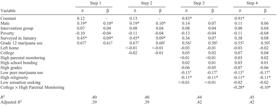 |
Notes: Outcome variable and lagged-dependent variables are natural log transformed. Interaction terms are centered. Only significant interactions are shown in Step 4.
p < .05;
p < .01;
p < .001.
Figure 4.

Probe of the interaction between college status and parental monitoring for changes in marijuana frequency from 12th grade to the following fall
Discussion
In summary, these results suggest that both moving away from home and going to college were significantly related to increases in alcohol-use behaviors during the period immediately after high school but were not related to increases in marijuana use. These results for alcohol are consistent with those of other studies (e.g., Bachman et al., 1997; Gfroerer et al., 1997; White et al., 2005) and support our hypotheses. It has been argued that the college environment encourages heavy drinking (Presley et al., 2002). Alcohol is often available at college social functions and students often view college as a place to drink excessively (White and Jackson, 2004–2005). In addition, college students may have more freedom from responsibilities and less social control compared with those who work (White et al., 2005). We found, however, that leaving home was a stronger predictor of increases in drinking behavior than was college attendance, which is consistent with Bachman et al.’s (1997) conclusion that it is primarily the move away from home that contributes to the high rates of heavy drinking noted among college students. As hypothesized, those youths who went to college and left home increased their frequency of drinking more than those who stayed home, regardless of college attendance. Yet, those who left home and did not go to college also reported relatively higher levels of drinking and heavy episodic drinking in emerging adulthood than those who stayed home, although the increases they experienced were not as steep as those of college students who moved away. Thus, the combination of college and moving away appears to assert the greatest effect, although this interaction was significant for frequency of alcohol use but not heavy episodic drinking. Perhaps because heavy episodic drinking is often a weekend activity, it may not depend as much on the freedoms associated with college attendance. Our findings suggest that there may be aspects of the college environment, in addition to living arrangements, that confer risk for frequent drinking (e.g., altered peer norms, availability) (Presley et al., 2002; Slutske et al., 2004; Wood et al., 2004), although it is possible that these changes occurred during the summer before entrance into college (see Wood et al., 2004).
In contrast to our hypothesis, leaving home and attending college did not have direct or interactive effects on relative increases in marijuana use after graduation from high school. Whereas noncollege-bound youths reported more frequent marijuana use in high school than college-bound youth, emerging adults did not significantly increase their marijuana use as they entered college. This result contrasts with Bachman and colleagues’ (1997) finding that college students increased their marijuana use after high school more than their noncollege peers did, although the former still did not reach as high levels as the latter. The difference in findings may be due to historical reductions in marijuana use from the late 1980s and early 1990s (when Bachman’s data were collected) to the Year 2004 (when our data were collected). In fact, neither the college nor noncollege youths reported much increase in marijuana-use frequency from high school to 6 months later.
We had hypothesized that protective factors in high school would moderate the effects of college and living status on substance use. We found only 3 significant interactions of protective factors out of 36 that were tested, which is less than would be expected by chance. Therefore, caution is necessary when interpreting these interaction effects. Lower sensation seeking in high school moderated the positive impact of attending college on increases in the frequency of drinking and heavy episodic drinking. Numerous studies have found a strong association between sensation seeking and substance use among adolescents (Bates et al., 1985) and sensation seeking appears to be a relatively stable trait from adolescence to emerging adulthood (Arnett, 2005). Our results suggest that those youths who have lower sensation-seeking needs may not be as influenced to increase their drinking, even in an environment that encourages heavy drinking. Bates and Labouvie (1995) found that sensation-seeking needs and environmental factors (e.g., deviant peers) acted additively to increase sustained movement along problematic alcohol-use trajectories from adolescence into young adulthood. In our study, sensation seeking did not have a direct or interaction effect on marijuana use, which is surprising given that sensation seeking has been consistently related to drug use (Bates et al., 1985). Perhaps sensation seeking is related to experimenting with marijuana but, once tried, the effects of marijuana (e.g., increased self-attention; Zablocki et al., 1991) may not be as reinforcing for high sensation seekers as the effects of alcohol. Nevertheless, it may be important to target youths with high sensation-seeking needs for additional interventions before departure from high school or on entry to college.
We also found that parental monitoring moderated the effects of going to college on marijuana use and had a direct protective effect on increases in heavy episodic drinking. Parental monitoring was not related to frequency of alcohol use, perhaps because simply drinking is a more normative behavior than drinking heavily or using marijuana. Parental monitoring in high school has been found to influence a wide range of problem behaviors, including substance use (Bates and Labouvie, 1995; Schulenberg and Maggs, 2002; White and Jackson, 2004–2005), and Wood and colleagues (2004) found that the effects of parental monitoring on heavy drinking and related problems remained strong in late adolescence after graduation from high school. We found here that parental monitoring in high school continued to exert influence on heavy drinking after high school graduation and on marijuana use as youths entered college. As predicted by the SDM, higher levels of parental monitoring in high school may strengthen prosocial socialization in high school. This heightened prosocial socialization may, in turn, reduce seeking opportunities for illegal drugs and drinking. Thus, making parents aware of the importance of monitoring for reducing substance use after high school and strengthening parental monitoring in high school and during the transition to college may be important preventive targets.
In addition to parental monitoring, higher religiosity and having fewer friends who used alcohol and marijuana in the 12th grade had direct protective effects on increases in all the substance-use measures 6 months later, except that religiosity was not related to increases in heavy episodic drinking. These are the same factors that Bates and Labouvie (1995) found to be associated, either directly or indirectly, with less increases in alcohol use and related problems from adolescence into emerging adulthood. Our findings support the SDM and indicate that bonding to prosocial peers and involvement in prosocial activities and beliefs place youths on a prosocial pathway that includes less substance use. The mechanisms that account for these enduring effects remain undefined by our analyses, however. The SDM hypothesizes that strengthened prosocial involvement and beliefs in the high school developmental period lead youth to seek out prosocial opportunities and avoid antisocial opportunities in the post-high school environment (Catalano and Hawkins, 2002). Regardless of the mechanisms, the findings suggest that providing opportunities for involvement in conventional activities (e.g., attending religious services) and reducing the number of substance-using peers during high school might help reduce increases in substance use following high school.
Although several of the protective factors measured in the 12th grade had direct effects on frequency of substance use measured approximately 6 months later, none reduced the impact of moving away from home. Thus, the move away from parents is a strong risk factor for increases in drinking behavior during emerging adulthood.
The present study had several advantages over prior studies examining the effects of college attendance and living arrangements on substance use (e.g., Bachman et al., 1997; Gfroerer et al., 1997) because we collected prospective data across a short follow-up window from both those who did and did not go to college. Nevertheless, some limitations should be noted. First, excluding youths who had already made a transition to college or out of their parents’ home during their last year of high school may have reduced our power to find significant interaction effects. Further, we excluded some youths who had already dropped out of school before the 12th-grade survey, and these youths had reported significantly higher levels of substance use at that time. The present analyses thus eliminated some of the most problematic substance users. Second, we combined the intervention and control groups in these analyses; however, we controlled for intervention status, and it was not significantly related to changes in substance use during this transitional period. Third, this study did not take into account environmental factors during the transition that may have affected changes in drinking and drug use. For those who moved away from parents, for example, we did not control for living partners or accommodations (Harford et al., 2002). Fourth, by combining 2- and 4-year college students and full- and part-time students, we may have obscured potential effects of differing college environments or lifestyles (Slutske et al., 2004). In addition, the group of nonstudents comprised those working full time, part time, and not at all; thus, they varied in their levels of disposable income and life satisfaction (White et al., 2005). Last, the sample was predominantly white and came from one suburban community. Our findings need to be replicated in other, more diverse samples. Future studies with larger samples should distinguish between students and nonstudents in terms of living and working situations and should explore changes in use of drugs other than alcohol and marijuana. More research is also needed to examine the potential mechanisms that explain how protective factors measured in high school continue to exert influence on substance use after high school.
Acknowledgments
The authors thank Erich Labouvie and two anonymous reviewers for their comments on this article and Grace Yan for her help with manuscript preparation.
Footnotes
The writing of this article was supported by National Institute on Drug Abuse grants DA08093 and DA17552.
References
- Aiken LS, West SG. Multiple Regression: Testing and Interpreting Interactions. Thousand Oaks, CA: Sage; 1991. [Google Scholar]
- Arnett JJ. Emerging adulthood: A theory of development from the late teens through the twenties. Amer Psychol. 2000;55:469–480. [PubMed] [Google Scholar]
- Arnett JJ. The developmental context of substance use in emerging adulthood. J Drug Issues. 2005;35:235–254. [Google Scholar]
- Bachman JG, Wadsworth KN, O’Malley PM, Johnston LD, Schulenberg JE. Smoking, Drinking and Drug Use in Young Adulthood: The Impacts of New Freedoms and New Responsibilities. Mahwah, NJ: Lawrence Erlbaum; 1997. [Google Scholar]
- Baer JS, Kivlahan DR, Marlatt GA. High-risk drinking across the transition from high school to college. Alcsm Clin Exp Res. 1995;19:54–61. doi: 10.1111/j.1530-0277.1995.tb01472.x. [DOI] [PubMed] [Google Scholar]
- Bates ME, Labouvie EW. Personality-environment constellations and alcohol use: A process-oriented study of intraindividual change during adolescence. Psychol Addict Behav. 1995;9:23–35. [Google Scholar]
- Bates ME, Labouvie EW. Adolescent risk factors and the prediction of persistent alcohol and drug use into adulthood. Alcsm Clin Exp Res. 1997;21:944–950. [PubMed] [Google Scholar]
- Bates ME, Labouvie EW, White HR. The effect of sensation seeking needs on changes in drug use during adolescence. Bull Social Psychol Addict Behav. 1986;5:29–36. [Google Scholar]
- Bingham CR, Shope JT, Tang X. Drinking behavior from high school to young adulthood: Differences by college education. Alcsm Clin Exp Res. 2005;29:2170–2180. doi: 10.1097/01.alc.0000191763.56873.c4. [DOI] [PMC free article] [PubMed] [Google Scholar]
- Borsari B, Carey KB. Peer influences on college drinking: A review of the research. J Subst Abuse. 2001;13:391–424. doi: 10.1016/s0899-3289(01)00098-0. [DOI] [PubMed] [Google Scholar]
- Brown EC, Catalano RF, Fleming CB, Haggerty KP, Abbott RD. Adolescent substance use outcomes in the Raising Healthy Children Project: A two-part latent growth curve analysis. J Cons Clin Psychol. 2005;73:699–710. doi: 10.1037/0022-006X.73.4.699. [DOI] [PubMed] [Google Scholar]
- Catalano RF, Hawkins JD. The social development model: A theory of antisocial behavior. In: Hawkins JD, editor. Delinquency and Crime: Current Theories. New York: Cambridge Univ. Press; 1996. pp. 149–197. [Google Scholar]
- Catalano RF, Hawkins JD. Response from authors to comments on “Positive youth development in the United States: Research findings on evaluation of positive youth development programs. Prev Treat. 2002;5:20. [Google Scholar]
- Catalano RF, Mazza JJ, Harachi TW, Abbott RD, Haggerty KP, Fleming CB. Raising healthy children through enhancing social development in elementary school: Results after 1.5 years. J School Psychol. 2003;41:143–164. [Google Scholar]
- Catalano RF, Park J, Harachi TW, Haggerty KP, Abbott RD, Hawkins JD. Mediating the effects of poverty, gender, individual characteristics, and external constraints on antisocial behavior: A test of the social development model and implications for developmental life-course theory. In: Farrington DP, editor. Advances in Criminological Theory, Vol. 14: Integrated Developmental and Life-Course Theories of Offending. New Brunswick, NJ: Transaction; 2005. pp. 93–123. [Google Scholar]
- Crowley JE. Educational status and drinking patterns: How representative are college students? J Stud Alcohol. 1991;52:10–16. doi: 10.15288/jsa.1991.52.10. [DOI] [PubMed] [Google Scholar]
- Darke S. Self-report among injecting drug users: A review. Drug Alcohol Depend. 1998;51:253–263. doi: 10.1016/s0376-8716(98)00028-3. [DOI] [PubMed] [Google Scholar]
- Dawson DA, Grant BF, Stinson FS, Chou PS. Another look at heavy episodic and alcohol use disorders among college and noncollege youth. J Stud Alcohol. 2004;65:477–488. doi: 10.15288/jsa.2004.65.477. [DOI] [PubMed] [Google Scholar]
- Finkel SE. Causal Analysis with Panel Data. Thousand Oaks, CA: Sage; 1995. [Google Scholar]
- Gfroerer JC, Greenblatt JC, Wright DA. Substance use in the US college-age population: Differences according to educational status and living arrangement. Amer J Publ Hlth. 1997;87:62–65. doi: 10.2105/ajph.87.1.62. [DOI] [PMC free article] [PubMed] [Google Scholar]
- Goldman MS, Boyd GM, Faden V, editors. J Stud Alcohol. Supplement No 14. 2002. College Drinking, What It Is, and What To Do about It: A Review of the State of the Science. [Google Scholar]
- Haggerty KP, Catalano RF, Harachi T, Abbott RD. Description de l’implantation d’un programme de prévention des problèmes de comportement à l’adolescence (Preventing adolescent problem behaviors: A comprehensive intervention description) Criminologie. 1998;31:25–47. [Google Scholar]
- Harford TC, Muthén BO. Alcohol use among college students: The effects of prior problem behaviors and change of residence. J Stud Alcohol. 2001;62:306–312. doi: 10.15288/jsa.2001.62.306. [DOI] [PubMed] [Google Scholar]
- Harford TC, Wechsler H, Muthén BO. The impact of current residence and high school drinking on alcohol problems among college students. J Stud Alcohol. 2002;63:271–279. doi: 10.15288/jsa.2002.63.271. [DOI] [PubMed] [Google Scholar]
- Hawkins JD, Catalano RF, Miller JY. Risk and protective factors for alcohol and other drug problems in adolescence and early adulthood: Implications for substance-abuse prevention. Psychol Bull. 1992;112:64–105. doi: 10.1037/0033-2909.112.1.64. [DOI] [PubMed] [Google Scholar]
- Jackson KM, Sher KJ, Park A. Drinking among college students: Consumption and consequences. In: Galanter M, editor. Recent Developments in Alcoholism, Vol. 17: Alcohol Problems in Adolescents and Young Adults. New York: Kluwer Academic/Plenum; 2005. pp. 85–117. [DOI] [PubMed] [Google Scholar]
- Johnston LD, O’Malley PM, Bachman JG, Schulenberg JE. Monitoring the Future: National Survey Results on Drug Use, 1975–2003, Vol. 1, NIH Publication No. 04-5507. Bethesda, MD: Department of Health and Human Services; 2004. [Google Scholar]
- Kerr M, Stattin H. What parents know, how they know it, and several forms of adolescent adjustment: Further support for a reinterpretation of monitoring. Devel Psychol. 2000;36:366–380. [PubMed] [Google Scholar]
- Menard S. Longitudinal Research. Thousand Oaks, CA: Sage; 1991. [Google Scholar]
- Needle R, McCubbin HI, Lorence J, Hochhauser M. Reliability and validity of adolescent self-reported drug use in a family-based study: A methodological report. Int J Addict. 1983;18:901–912. doi: 10.3109/10826088309033058. [DOI] [PubMed] [Google Scholar]
- Newcomb MD, Abbott RD, Catalano RF, Hawkins JD, Battin-Pearson S, Hill K. Mediational and deviance theories of late high school failure: Process roles of structural strains, academic competence, and general versus specific problem behavior. J Counsel Psychol. 2002;49:172–186. [Google Scholar]
- Newcomb MD, Bentler PM. Changes in drug use from high school to young adulthood: Effects of living arrangement and current life pursuit. J Appl Devel Psychol. 1987;8:221–246. [Google Scholar]
- Peterson PL, Hawkins JD, Abbott RD, Catalano RF. Disentangling the effects of parental drinking, family management, and parental alcohol norms on current drinking by black and white adolescents. J Res Adolesc. 1994;4:203–227. [Google Scholar]
- Petrie R, Fleming C, Haggerty K, Catalano Harachi T, Brown E. Asking 18 year olds about sex and drugs: A comparison of web and in-person survey modes. Poster presented at the annual meetings of the Society of Prevention Review; Washington, DC. May 26, 2005. [Google Scholar]
- Presley CA, Meilman PW, Leichliter JS. College factors that influence drinking. J Stud Alcohol. 2002;(Supplement No 14):82–90. doi: 10.15288/jsas.2002.s14.82. [DOI] [PubMed] [Google Scholar]
- Rae-Grant N, Thomas BH, Offord DR, Boyle MH. Risk, protective factors, and the prevalence of behavioral and emotional disorders in children and adolescents. J Amer Acad Child Adolesc Psychol. 1989;28:262–268. doi: 10.1097/00004583-198903000-00019. [DOI] [PubMed] [Google Scholar]
- Rutter M. Psychosocial resilience and protective mechanisms. In: Rolf JE, Masten AS, Cicchetti D, Nuechterlein KH, Weintraub S, editors. Risk and Protective Factors in the Development of Psycho-pathology. New York: Cambridge Univ Press; 1990. pp. 181–214. [Google Scholar]
- Schulenberg JE, Maggs JL. A developmental perspective on alcohol use and heavy drinking during adolescence and the transition to young adulthood. J Stud Alcohol. 2002;(Supplement No 14):54–70. doi: 10.15288/jsas.2002.s14.54. [DOI] [PubMed] [Google Scholar]
- Sheffield FD, Darkes J, Del Boca FK, Goldman MS. Binge drinking and alcohol-related problems among community college students: Implications for prevention policy. J Amer Coll Hlth. 2005;54:137–141. doi: 10.3200/JACH.54.3.137-142. [DOI] [PubMed] [Google Scholar]
- Slutske WS, Hunt-Carter EE, Nabors-Oberg RE, Sher KJ, Bucholz KK, Madden PAF, Anokhin A, Heath AC. Do college students drink more than their non-college-attending peers? Evidence from a population-based longitudinal female twin study. J Abnorm Psychol. 2004;113:530–540. doi: 10.1037/0021-843X.113.4.530. [DOI] [PubMed] [Google Scholar]
- Steinberg L, Fletcher A, Darling N. Parental monitoring and peer influences on adolescent substance use. Pediatrics. 1994;93:1060–1064. [PubMed] [Google Scholar]
- Steinman KJ, Zimmerman MA. Religious activity and risk behavior among African American adolescents: Concurrent and developmental effects. Amer J Commun Psychol. 2004;33:151–161. doi: 10.1023/b:ajcp.0000027002.93526.bb. [DOI] [PubMed] [Google Scholar]
- Stouthamer-Loeber M, Loeber R, Wei E, Farrington DP, Wilkstrom POH. Risk and promotive effects in the explanation of persistent serious delinquency in boys. J Cons Clin Psychol. 2002;70:111–123. doi: 10.1037//0022-006x.70.1.111. [DOI] [PubMed] [Google Scholar]
- Stouthamer-Loeber M, Wei E, Loeber R, Masten AS. Desistance from persistent serious delinquency in the transition to adulthood. Devel Psychopathol. 2004;16:897–918. [PubMed] [Google Scholar]
- Wallace JM, Jr, Brown TN, Bachman JG, LaVeist TA. The influence of race and religion on abstinence from alcohol, cigarettes and marijuana among adolescents. J Stud Alcohol. 2003;64:843–848. doi: 10.15288/jsa.2003.64.843. [DOI] [PubMed] [Google Scholar]
- Wechsler H, Lee JE, Kuo M, Lee H. College binge drinking in the 1990s: A continuing problem: Results of the Harvard School of Public Health 1999 College Alcohol Study. J Amer Coll Hlth. 2000;48:199–210. doi: 10.1080/07448480009599305. [DOI] [PubMed] [Google Scholar]
- White HR, Jackson K. Social and psychological influences on emerging adult drinking behavior. Alcohol Res Hlth. 2005;28:182–190. [Google Scholar]
- White HR, Labouvie EW, Papadaratsakis V. Changes in substance use during the transition to adulthood: A comparison of college students and their noncollege age peers. J Drug Issues. 2005;35:281–306. [Google Scholar]
- Wood MD, Read JP, Mitchell RE, Brand NH. Do parents still matter? Parent and peer influences on alcohol involvement among recent high school graduates. Psychol Addict Behav. 2004;18:19–30. doi: 10.1037/0893-164X.18.1.19. [DOI] [PubMed] [Google Scholar]
- Zablocki B, Aidala A, Hansell S, White HR. Marijuana use, introspectiveness, and mental health. J Hlth Social Behav. 1991;32:65–79. [PubMed] [Google Scholar]