Interleaved concatenated codes: New perspectives on approaching the Shannon limit

Abstract

The last few years have witnessed a significant decrease in the gap between the Shannon channel capacity limit and what is practically achievable. Progress has resulted from novel extensions of previously known coding techniques involving interleaved concatenated codes. A considerable body of simulation results is now available, supported by an important but limited theoretical basis. This paper presents a computational technique which further ties simulation results to the known theory and reveals a considerable reduction in the complexity required to approach the Shannon limit.

Nearly 50 years ago, Claude Shannon published a series of remarkable theoretical results (1–3), which ever since have served as a beacon and goal for digital communication researchers. Among the better-known aspects of this work is a formula for the “channel capacity” of a wireless propagation channel of a given bandwidth perturbed by additive thermal noise: specifically, that this capacity, measured in bits/sec received, is linearly proportional to the bandwidth and logarithmically proportional to the received signal-to-noise ratio. Far more important than Shannon’s channel capacity formula (3), however, is its significance: namely, that it is possible to process the information prior to transmission (encoding) and after reception (decoding) so as to achieve error-free communication asymptotically, as processing load and memory size approach infinity, provided the transmission rate (in bits/sec) does not exceed the channel capacity; conversely, for transmission rates above channel capacity, error-free communication becomes impossible and, in fact, error probability approaches unity for the same processing techniques for which it approaches zero at rates below capacity.

There remained to determine specific, and preferably practical, means for achieving near error-free communication. Early attempts at constructing encoders and decoders which could provide performance approaching Shannon’s channel capacity were through application of finite-field algebraic concepts. While these have led to some powerful means for error correction and detection in computers and storage devices, some of which have had major influences on the economics of recording (4), their impact on the central goal of approaching capacity, particularly for wireless and other physical channels, has been minor.

Considerable progress, on the other hand, has resulted from a seemingly nonconstructive approach, referred to generally as “random coding” (5). Channel coding theory actually addresses three related problems:

(i) construction of codes which will result in a low error probability on the given channel;

(ii) implementation of an optimal (maximum likelihood) or near optimal decoder for these codes; and

(iii) performance analysis to determine error probabilities for these codes, decoders, and channels.

The random coding approach bypasses problem i by considering the ensemble of all possible codes constructed from a given symbol alphabet of a particular block length and code rate. Then for a maximum likelihood decoder, which achieves ii, it determines the average error probability for the ensemble of all possible codes with the given parameters; at least one code in this ensemble must perform better than this average, thus establishing an upper bound on the error probability of a desirable code, which is what is sought in problem iii.

Traditional Error Bounds

Suppose K information bits are encoded into a sequence of symbols which are in turn transformed into physical signals to be transmitted over a physical channel. The performance of this so-called block code on a particular channel is measured by the probability of an error in deciding, based on the signal received, that a particular (incorrect) K-bit block was sent rather than the (correct) block which was actually sent. The computation of an upper bound on this error probability is achieved, as noted above, by computing the ensemble average over all possible codes, which may be used to represent all possible K-bit blocks. It is further facilitated, though weakened, by employing the well known union bound

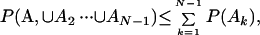where A_k in this case represents the error event that the kth incorrect block is chosen in place of the correct one, where k takes on one of N − 1 = 2^K − 1 values. With these two simplifications (ensemble average of the union bound), for most physical channels, the error probability bound is readily computed as

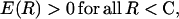
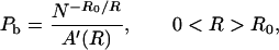
where R is the transmission rate in bits/channel symbol and R₀, known as the “computational cutoff rate,” is solely a function of the channel. R₀ is never greater than capacity, and for all physical channels it is strictly less, and clearly the bound becomes useless at R = R₀. However, the union bound can be improved in such a way that, after averaging over the code ensemble, it yields the tighter bound,

whose exponent is asymptotically tight for all but low rates and approaches zero as rate, R, approaches capacity, C. Even so, the result is discouraging, since a receiver employing a maximum likelihood decoding algorithm generally must perform N = 2^K operations, one for each codeword, so that in terms of the complexity N,

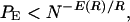where the exponent E(R)/R → 0 as R → C, and even at R = R₀ < C, the exponent is typically considerably smaller than unity.

A brighter picture emerges for the class of nonblock codes known as convolutional codes, which are linearly generated by a shift register of K_c − 1 stages, where K_c is known as the constraint length of the code (see Fig. 1a for an example with K_c = 3). The ensemble average of union bounds on bit error probability† over all codes of this class for a given R and K_c is

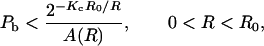where A(R) > 0 for R < R₀ independent of K_c.

Figure 1.

Rate 1/2, 4-state convolutional codes.

If the union bound is improved in the same manner as for block codes, we obtain

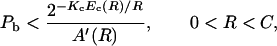where A′(R) > 0 for R < C,

and the exponent is asymptotically tight for R₀ ≤ R < C.

Since a convolutional encoder is just a finite state machine, the number of operations required per bit just equals the number of connections between all possible successive states, which is proportional to 2^K_c. Thus in terms of complexity

which means that, even at R = R₀, bit error probability is inversely proportional to complexity.

In practical terms, to achieve bit error probabilities on the order of 10⁻⁶, with a complexity on the order of 10³ operations/bit, one has to select R somewhat below R₀. Since the bounds are slightly pessimistic, the backoff for convolutional codes needs only to be on the order of R = (3/4)R₀. The parameter of interest for physical wireless channels characterized by line-of-sight propagation and thermal noise or broadband Gaussian noise or interference (e.g., satellite channels) is the bit energy-to-noise density ratio, E_b/N₀. For such channels with binary phase shift keyed modulation,

so that

Choosing R = 1/2, corresponding to a convolutional code such as that shown in Fig. 1 (but with K_c = 9, instead of K_c = 3), taking R₀ = 2/3 as noted above, we obtain E_b/N₀ = 2.7 [or 4.3 decibel (dB)]. Note that with no constraints on modulation, the channel capacity is (3)

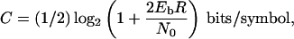so that at R = C = 1/2 bits/symbol, E_b/N₀ = 1 or (0 dB), while at R = R₀ = 1/2, E_b/N₀ = 2.5 dB.

Thus state-of-the-art codes‡ operate at E_b/N₀ nearly 2 dB above the value corresponding to R₀ and nearly 4 dB above that corresponding to channel capacity; this corresponds to a rate about 40% of capacity. Both theorists and practitioners were satisfied with this state of affairs until a very few years ago, when a new perspective showed that improvements in rate up to a factor of 2 were possible without an increase in complexity.

New Perspectives: Interleaved Concatenated Codes

Beginning in 1993 (6), a number of empirical results based mostly on simulations perturbed the status quo of the well established theory, which for several decades had been the accepted basis for finding and evaluating effective codes for transmission over noisy channels. Without dwelling on the various steps in the evolution of this new approach (7–9), we shall describe its currently most promising embodiment (10) and provide a few theoretical and computational justifications for the marked advantages which it provides. The coding structure shown in Fig. 2 is known as an interleaved concatenated code, with a first level of coding which operates on K input bits to produce N code symbols (usually binary); following this is an interleaver, which reorders the N code symbols according to some arbitrary permutation; the N symbols are then operated on by a second coder to generate J output symbols, which are used to modulate the transmitter. K < N < J and the rates of the two encoders are, respectively, K/N and N/J bits/symbol, so that the overall concatenated code rate is K/J bits/symbol. Somewhat surprisingly, this concatenated structure has a long history in the coding literature, having been developed and applied for over 30 years (11, 12). The recent contributions introduce certain new characteristics in the implementation of the encoders and interleaver, and particularly of the decoding process, which render possible much improved performance over the conventional and historical implementation, without increased complexity.

Figure 2.

(Serially) concatenated codes.

Conventional Codes.

To understand the impact of these novel processors, which are generally labeled “turbo” coders and decoders, it is useful to review briefly the implementation and evaluation of a conventional code, which can also be used as one of the component codes of the concatenated system. Although the above description implies block codes, of K and N input bits, respectively, each can be implemented as a truncated convolutional code. Referring to Fig. 1a, this is accomplished by starting in a known state (e.g., all stages of the shift register containing zeros) and also ending in a known (possibly the same) state. This requires terminating the (K or N) bit block with a non-information-bearing sequence of K_c − 1 known bits, called the “tail.”

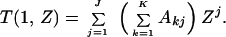
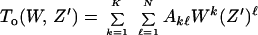
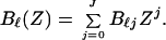
A union bound on the error probability of such a (terminated convolutional) block code operating on the additive Gaussian noise channel is obtained from a generating function called the input–output weight enumeration function (IOWEF) (10). For a particular code of K input bits and J output symbols, this is a two-dimensional polynomial

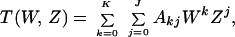1

where A_kj is the number of codewords generated by k (out of a possible K) input ones which produce j output ones; that is, for which k and j are, respectively, the input and output (Hamming) weights of the codeword. Because the encoder is just a finite-state machine, this generating function is readily obtained from the one-stage transition matrix of the encoder, C(W, Z), which is illustrated in Fig. 1a for the convolutional code example therein. The states are labeled in increasing order and the matrix refers to the augmentation of input and output weights resulting from one bit of the input sequence. Thus if i is the state of the coder register after n − 1 bits have been input to the coder and S⁽ⁱ⁾ (n − 1) is the corresponding IOWEF for a codeword generated by these first n − 1 input bits, then the S_n⁽ⁱ⁾ corresponding IOWEF after n input bits is obtained by the recursion:

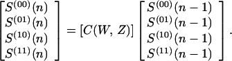2

Generalization to any constraint length K_c, with 2^K_c−1 state equation is obvious. From this it follows that the complete IOWEF after K input bits beginning in state (00) is obtained by K iterations of Eq. 2 from the initial state vector

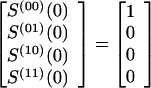3

to the Kth state vector, which is obtained by K successive matrix multiplications to be

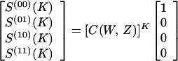4

Thus for an ending state i = (00), the IOWEF of Eq. 1 is obtained from the first term of Eq. 4 as

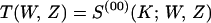5

the all-zero state (zeros in both, or more generally, all memory elements). This is all that is needed to obtain a union bound on bit error probability.

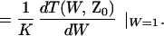
From a computational viewpoint, as simple as these expressions seem, the polynomial multiplications become unwieldy and increasingly burdensome for increasing N, even for a symbolic manipulation program. On the other hand, we may obtain upper bounds on block and bit error probabilities from the IOWEF by setting numerical values for W and Z, in which case all operations become numerical. In particular, letting W = 1 in Eq. 1,

But because A_kj is the total number of codewords of input weight k and output weight j, then ∑_k=1^KA_kj is the total number of codewords of weight j. The union bound on block error probability is just the sum of pairwise error probabilities; for a linear code the pairwise error probability between two codewords which differ in j output symbols may be upper bounded by Z₀^j where Z₀ depends only on the channel parameters. For a Gaussian channel with binary inputs, Z₀ = e^−E_s/N₀ = e^−RE_b/N₀, where E_s is the symbol energy, E_b is the corresponding bit energy, and R is the code rate (13). Consequently, the block error probability is upper bounded by

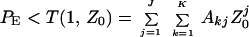6

The bit error probability, on the other hand, depends on the number of input bits as well as the number of output bits that differ. It is readily shown, with the same arguments, that

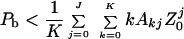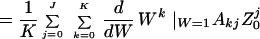7

The derivative can be obtained numerically, and slightly further upper bounded by using, for ɛ very small,

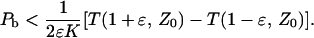Interleaved Concatenated Codes.

We turn now to applying the same computational approach for concatenated codes. Referring again to Fig. 2, let

be the IOWEF of the first (outer§) code and

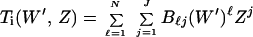be the IOWEF of the second (inner§) code.

Any one output sequence of the outer coder of weight ℓ, which is input to the inner coder, will produce one output sequence. But if we consider all sequences of weight ℓ output from the outer coder and input to the inner (which we shall henceforth call “middle” sequences), we obtain, overall, a number A_kℓB_ℓj sequences which have input weight k and output weight j, and middle weight ℓ. Since the length of the middle sequence is N, there are (_ℓ^N) distinct permutations of sequences of weight ℓ. Thus, assuming that a particular permutation is chosen randomly with uniform probability by the interleaver, we obtain for the ensemble average IOWEF of the concatenated code,

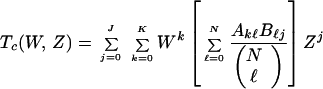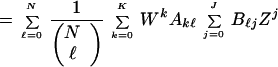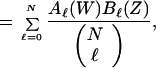8

where

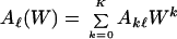9

and

10

Using Eqs. 6 and 7, we obtain the ensemble average concatenated block error probability over all equally probable interleaver permutations,

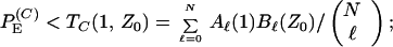11

and similarly the concatenated bit error probability ensemble average

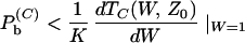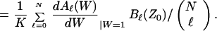12

Computation of A_ℓ(W) and B_ℓ(Z), for numerical values of W and Z, can proceed in a manner similar to T(W, Z) of Eq. 5, but adjusted to eliminate the alternative variable. The method is illustrated in the Appendix.

Using for the outer code the constraint length 3 convolutional code of Fig. 1a and for the inner code the code of Fig. 1b, we obtain the numerical results of Fig. 4a. For comparison (prompted by a theoretical result discussed in the last section) in Fig. 4b we substitute the K = 5 outer code of Fig. 3 for that of Fig. 1a but use the same inner code of Fig. 1b. In light of the discussion of the conventional coding performance results at the end of the last section, these results are quite remarkable. With extremely short component codes, each of which would require E_b/N₀ > 6 dB to attain error probabilities below 10⁻⁵ (13), the concatenated code attains very low error probabilities at E_b/N₀ < 2 dB and the level seems to decrease rapidly as the interleaver size increases. Note from the expression for E_b/N₀ in terms of R₀ and R in the Traditional Error Bounds section, that for the compound rate R = 1/4, setting R₀ = R corresponds to E_b/N₀ = 1.85 dB. Thus, it appears that the error probability can be made as small as desired for all rates up to R₀ (or equivalently for all E_b/N₀ greater than the value corresponding to R = R₀) simply by increasing the interleaver and hence the block length.

Figure 4.

BER for rate 1/4 concatenated code. (a) Rate 1/2, 4-state inner and outer codes. (b) Sixteen-state outer, 4-state inner codes.

Figure 3.

Alternate outer coder (16 states).

We shall describe some theoretical underpinnings for this behavior in the last section. First we must consider the decoder.

Decoder Implementation

The gap in the results just presented concerns the decoder implementation. The above assumed a maximum likelihood decoder for the entire code, which can become overly complex, almost as much as for an ordinary block code of K input bits. The conventional, and much less complex, decoder for a concatenated code first decodes the inner code (nearest the channel), and then feeds its input bit decisions to the outer decoder, which proceeds to decode so as to decide on the original user inputs. This approach yields very mediocre results. Better performance is achieved with a “soft output” decoder for the inner code (14, 15). Rather than making a definitive decision on the bits encoded by the inner coder, the inner decoder outputs to the outer decoder “soft decisions,” meaning that it provides, along with the decisions, a metric related to the a posteriori probabilities that these decisions are correct. Even better performance is achieved by an “iterative soft decision” decoder. This refers to a decoder that not only furnishes soft decisions regarding the inner decoder inputs to the outer decoder but also performs soft decisions on the code symbols output from the outer decoder, which are input to the inner decoder; it then repeats the inner decoding operation, followed by the outer decoding, and so forth, in each case providing soft decisions to the other for the next step. This procedure can continue for arbitrarily many steps, each time improving the estimate of each. After n iterations, the outer decoder finally outputs a final decision on each of the input bits.

Current State of Development: Theoretical, Computational, and Empirical

When “turbo” codes were first presented¶ in 1993 by Berrou et al. (6), results were based solely on simulations. Given their impressive improvement in performance over conventional codes, the results were met with considerable skepticism in many quarters. Today that skepticism has been fully dispelled by extensive supporting evidence involving a combination of theoretical, computational, and simulation results, which we summarize in that order.

Theoretical.

Benedetto et al. (10) have shown that under the condition that the inner coder is recursive, every term of the union bounds 11 and 12 is proportional to N^−α, where α is a positive integer.

13

14

where Int[x] is the integer part of x and d_f^(o) is the free distance (minimum weight) of the outer convolutional code. Further, they have shown that if the inner code is nonrecursive, the error probability may instead grow with N.

Computational.

Regrettably, there are no closed-form expressions for bounds similar to those for conventional codes as given in the Traditional Error Bounds section. However, the computational techniques described in the New Perspectives section produce conclusive evidence that interleaved concatenated codes can produce extremely low error probabilities for rates below R₀ (or E_b/N₀ above the value corresponding to R = R₀). Fig. 4 verifies the strong effect of increasing N. In fact, it is readily apparent that the bounds of Fig. 4a behave as N⁻³ and those in Fig. 4b as N⁻⁴. This corroborates the theoretical result of the preceding paragraph, since the outer codes of Fig. 1a and Fig. 3 have d_f^(o) = 5 and d_f^(o) = 7, respectively, which, according to expressions 13 and 14, implies α = 3 and 4, respectively.

Simulation.

To justify using the iterative soft decision decoding technique described in the Decoder Implementation section, as well as to obtain results for rates between R₀ and C (corresponding to low E_b/N₀), there is as yet no alternative to simulation. However, with the theoretical underpinnings and computational evidence, the simulations are clearly validated. For example, the simulation results shown in Fig. 4b, for an iterative decoder performing 8 iterations, demonstrate acceptable performance for E_b/N₀ lower than the region covered by the bounds, which appears to corroborate the bounds at least in its rate of approach thereto. (Simulations of error possibilities below 10⁻⁸ require prohibitively large samples.)

To summarize the state of knowledge, there are two predominant questions which are yet to be fully answered:

(i) How close to the optimum overall maximum likelihood decoder performance is that of the iterative soft decision decoder?

(ii) How close to capacity can the above codes and decoders operate with reasonable performance?

Extensive simulations, with interleaver memories as large as N = 2¹⁶ (65,536), indicate for the latter that E_b/N₀ within less than 1 dB (rates to within 80%) of capacity can be achieved.

While theoretical support for these important issues is still lacking, one major conclusion is now well supported: excellent performance, well beyond what was previously considered practically achievable, is obtainable with quite moderate complexity (which is proportional to the number of decoding iterations required). This performance thus depends only very weakly on complexity but strongly on the interleaving memory size and hence the decoding delay. Coincidentally, this supports the fundamentals of Shannon theory. Only the traditional reliance on exponential error bounds is eclipsed by these conclusions.

ABBREVIATIONS

dB

decibel

IOWEF

input–output weight enumeration function

Appendix

We demonstrate the procedure for recursively computing A_ℓ(W) and B_ℓ(Z) of Eqs. 9 and 10, using the example of a concatenated code consisting of the outer code of Fig. 1a and the inner code of Fig. 1b. Since A_ℓ is a weighted sum of coefficients of the IOWEF for which the outer code has exactly ℓ output ones, we may recursively compute this based on the state recursion 2 as applied to the encoder in question. From Fig. 1a we may write the recursion equation for the outer code as

A.1

where A_ℓ⁽⁰⁰⁾N/2 = A_ℓ represents‖ the weighted sum which we desire, while A_ℓ^(s)(n) for s ≠ 00 is the corresponding function for a code which arrives at state (s) at time n. Since the encoder is assumed to start in the all-zeros state, the initial conditions for the A_ℓ^(s) vector are

A.2

Similarly, for the inner code of Fig. 1b we have the recursions for B_ℓ^(s)(n) with B_ℓ⁽⁰⁰⁾(N) = B_ℓ which represents the weighted sum of IOWEF coefficients for which the inner code has exactly ℓ input ones,

A.3

with initial conditions

A.4

Similar recursions apply for any convolutional code and are derived from its transfer matrix [C(Z, W)]. We note finally that the computational load for an N-symbol interleaver and an S state component code (inner or outer) is on the order of N²S².

While in principle the results of Eqs. A.1 and A.3 yield the necessary terms to compute numerically the codeword and bit error probability bounds of Eqs. 11 and 12, there remains one thorny issue. Both the terms of the recursions and the normalizing factor (_ℓ^N) become very large very quickly. To prevent overflows, it is necessary to normalize at each step of both recursions. This is facilitated by noting the equality

Thus, multiplying the ℓth term by (1 − ℓ/n) on the nth iteration provides the normalization and avoids overflow. Note, however, that since two separate recursions are performed, each should be multiplied by a fractional power of (1 − ℓ/n) with the two powers summing to unity.

References

- 1.Shannon C E. Bell System Tech J. 1948;27:379–423. [Google Scholar]
- 2.Shannon C E. Bell System Tech J. 1948;27:623–656. [Google Scholar]
- 3.Shannon C E. Proc IRE. 1949;37:10–21. [Google Scholar]
- 4.Berlekamp E R. Proc IEEE. 1980;68:564–593. [Google Scholar]
- 5.Gallager R G. IEEE Trans Inf Theory. 1965;IT-11:3–18. [Google Scholar]
- 6.Berrou C, Glavieux A, Thitimajshima P. IEEE International Conference on Communications, Geneva, Switzerland. Los Alamitos, CA: IEEE Press; 1993. pp. 1064–1070. [Google Scholar]
- 7.Hagenauer J, Hoeher P. IEEE Globecom, Dallas, TX. Los Alamitos, CA: IEEE Press; 1989. pp. 47.1.1–47.1.7. [Google Scholar]
- 8.Benedetto S, Montorsi G. IEEE Trans Inf Theory. 1996;42:409–428. [Google Scholar]
- 9.Hagenauer J, Offer E, Papke L. IEEE Trans Inf Theory. 1996;42:429–445. [Google Scholar]
- 10.Benedetto S, Montorsi G, Divsalar D, Pollara F. TDA Progress Report 42–126. Pasadena, CA: Jet Propulsion Laboratory; 1996. pp. 1–26. [Google Scholar]
- 11.Forney G D. Concatenated Codes. Cambridge, MA: MIT Press; 1967. [Google Scholar]
- 12.Lin S, Costello D J. Error Control Coding Fundamentals and Applications. Englewood Cliffs, NJ: Prentice Hall; 1983. [Google Scholar]
- 13.Viterbi A J, Omura J K. Principles of Digital Communication and Coding. New York: McGraw-Hill; 1979. [Google Scholar]
- 14.Benedetto S, Montorsi G, Divsalar D, Pollara F. TDA Progress Report 42–124. Pasadena, CA: Jet Propulsion Laboratory; 1995. pp. 63–87. [Google Scholar]
- 15.Benedetto S, Divsalar D, Montorsi G, Pollara F. TDA Progress Report 42–127. Pasadena, CA: Jet Propulsion Laboratory; 1996. pp. 1–20. [Google Scholar]