Reproducing Kernel Hilbert Spaces Regression Methods for Genomic Assisted Prediction of Quantitative Traits

Abstract

Reproducing kernel Hilbert spaces regression procedures for prediction of total genetic value for quantitative traits, which make use of phenotypic and genomic data simultaneously, are discussed from a theoretical perspective. It is argued that a nonparametric treatment may be needed for capturing the multiple and complex interactions potentially arising in whole-genome models, i.e., those based on thousands of single-nucleotide polymorphism (SNP) markers. After a review of reproducing kernel Hilbert spaces regression, it is shown that the statistical specification admits a standard mixed-effects linear model representation, with smoothing parameters treated as variance components. Models for capturing different forms of interaction, e.g., chromosome-specific, are presented. Implementations can be carried out using software for likelihood-based or Bayesian inference.

A massive quantity of genomic information is increasingly available for several species. For example, Wong et al. (2004) reported 2.8 million single-nucleotide polymorphisms (SNPs) in the chicken genome, and Hayes et al. (2004) found 2507 putative SNPs in salmons. Hundreds of thousands of SNPs have been identified in humans (e.g., Hartl and Jones 2005). It is natural to consider use of this information as an aid in genetic improvement of livestock or plants or in molecular classification (or prediction) of diseases. In medicine and agriculture, for example, genomic information could also be used for designing diet or plant fertilization regimes that are genotype specific.

Early discussions on the use of molecular markers in genetic selection programs are given by Soller and Beckmann (1982) and Fernando and Grossman (1989). Subsequently, much work has addressed determining location and use of a single or a few quantitative trait loci (QTL). However, Dekkers and Hospital (2002), in a review of many studies, observed that there are an abundant number of loci associated with variation in quantitative traits. These authors noted that most statistical methods for marker-assisted selection proposed so far do not deal adequately with the complexity (in the sense of number of loci) posed by many traits. A relevant issue to be addressed is how a massive number of SNPs, viewed as covariates with potential explanatory power, can be incorporated reasonably into a statistical model specification. Some hurdles in the process of model building include multiple testing, strong dependence of inferences on assumptions, ambiguous interpretation of effects in a multiple-marker analysis due to collinearity, the famous “curse of dimensionality,” as the number of markers, e.g., SNPs, exceeds by far the number of cases in a sample, and the handling of nonadditive gene action. Balding (2006) discusses many of these problems.

A main challenge is how the many interactions between genotypes at different loci ought to be dealt with. A stylized treatment of epistatic variability from an evolutionary perspective is presented by Cheverud and Routman (1995). Translating this into whole-genome data analysis is another matter: if thousands of marker genotypes are fitted in a model for genomic-assisted prediction, the number of potential interactions and their interpretation can be mind boggling.

First, consider an analysis with random-effects models, so that the variance component parameterization or, more generally, the dispersion structure becomes the focus of the problem. Due to smoothing or “regularization” induced by, e.g., a multivariate normal assumption, all random effects can be predicted uniquely. This is illustrated in Meuwissen et al. (2001), Gianola et al. (2003), and Xu (2003). For instance, animal breeders typically infer a number of breeding values that amply exceed the number of observations available (Quaas and Pollak 1980). However, coping with nonadditive genetic variability introduces additional difficulty. Theoretically, epistatic variance can be partitioned into orthogonal additive × additive, additive × dominance, dominance × dominance, etc., variance components, only under idealized conditions. These include linkage equilibrium, absence of mutation and of selection, and no inbreeding and assortative mating (Cockerham 1954; Kempthorne 1954). These assumptions are violated in nature and in breeding programs. Also, estimation of nonadditive components of variance is very difficult, even under standard assumptions (Chang 1988), leading to imprecise inference. Therefore, whether or not standard random-effects models for quantitative genetic analysis account for nonadditive relationships between genotypes and phenotypes accurately remains an open question.

Second, interactions between markers could be studied using fixed-effects models; this is what Cheverud and Routman (1995) refer to as “physiological epistasis,” to disassociate inference from the gene and genotype frequencies that generate a probability distribution. Such an analysis “runs out” of degrees of freedom quickly in a whole-genome treatment, because there are 2 d.f. per biallelic SNP locus. Even if the number of parameters is reduced in some manner, estimates of effects are expected to be unstable and imprecise, due to severe lack of orthogonality induced, partly, by extant linkage disequilibrium. Also, interactions involving more than three loci are very difficult to interpret. A standard parametric treatment may require a formidable model selection exercise, with any model in particular probably having little plausibility or predictive power. Bayesian model averaging (e.g., Hoeting et al. 1999) is an option, but how can this be made free from some strong and possibly untestable parametric assumptions?

A third and distinct avenue is to explore model-free approaches, which may be useful for phenotypic prediction under subtle or cryptic forms of epistasis. There is little evidence that such methods have been considered in quantitative genetics. Gianola et al. (2006) discussed semiparametric procedures for analysis of complex phenotypic data involving massive genomic information. These authors argued that application of the parametric additive genetic model in selective breeding of livestock produced tangible dividends, as shown in Dekkers and Hospital (2002), and proposed combining a nonparametric treatment of effects of molecular SNPs with features of the additive polygenic mode of inheritance.

The objective of this article is to develop further a reproducing kernel Hilbert spaces (RKHS) mixed model proposed by Gianola et al. (2006), with a focus on its theoretical aspects. The accompanying article by González-Recio et al. (2008, this issue) presents an application of the methodology to data on chicken mortality.

This article is organized as follows. The semiparametric mixed model section sets the stage and introduces notation. The nonparametric treatment (RKHS) adopted here is sketched in the reproducing kernel hilbert spaces regression section, where the main theoretical results are presented; additional details are in the appendix. dual formulation shows how the problem can be embedded into a mixed-effects model structure and discusses how statistical learning proceeds in a penalized-likelihood framework. The rkhs chromosome mixed model section presents a linear model aimed at capturing interactions between many loci at different chromosomes and presents a Bayesian implementation. The article concludes with a discussion of some standing issues.

SEMIPARAMETRIC MIXED MODEL

Setting:

The notation follows that of Gianola et al. (2006). Each of n individuals possesses a measurement for some quantitative trait denoted as y and information on a possibly massive number of SNP genotypes represented by a vector x. An SNP locus is considered biallelic, so at most three genotypes are observed. Genotype instances can be coded uniquely via two linearly independent variables per locus as in an analysis-of-variance setting, i.e., with 2 d.f. per locus. In standard quantitative genetics settings, the two dummy variates are coded such that the corresponding effects are interpretable as “additive” and “dominance.” This is irrelevant from the predictive point of view taken here, in the sense that parameters (most of which lack a mechanistic interpretation) serve as transition tools, to pass from observed to predicted data.

Suppose, temporarily, that there are no nuisance variables and that the focus is on discovering a function relating x_i to y_i. Three alternative modeling possibilities are considered, for illustrative purposes.

1. Let the relationship between y and x be represented as

   (1)

   where y_i is a measurement on the quantitative trait for individual i, x_i is a p × 1 vector of dummy SNP instance variates observed on i, and is some unknown function relating genotypes to phenotypes. Define as the conditional expectation function, that is, the mean phenotypic value of an infinite number of individuals, all possessing the p-dimensional genotypic attribute vector x_i. is a random residual, distributed independently of x_i and with variance . Typically, the residual distribution is assumed normal.

   The vector x may have a probability distribution reflecting frequencies of the SNP attributes in the population. However, the prediction problem normally centers on what can be expected about the phenotypic distribution, given some specific configuration x = x*, say. In nonparametric regression, is left unspecified and estimated as a smooth ; this function represents pertinent signals on the phenotype from elements of x_i, acting either additively or as members of some genetic network. Several techniques for inferring are described in Takezawa (2005).

2. A second specification is the additive regression model

   (2)

   (Hastie and Tibshirani 1990; Fox 2005), where x_ij is the value of attribute j in individual i. Each of the “partial-regression” functions allows exploration of effects of individual attributes on phenotypes. This model is expected to pick up additive and dominance effects at each of the marker loci, but not epistatic interactions. It does not possess any clear advantage over a standard regression model with additive and dominance effects, the main difference residing in the nonparametric treatment that (2) would receive.
3. One could also think in terms of an additive “chromosome” model, as follows. Let C be the number of pairs of chromosomes, and partition vector x_i as , so that contains the values of the SNP instance variates at chromosome pair j , and so on. If the number of SNPs in chromosome pair j = , then the order of x_ij is p_j, and the dimension of x is . The additive chromosome model is

   (3)

   with x_ij being the attributes observed on chromosome pair j for individual i. This model would account for chromosome-specific signals (reflecting additive, dominance, and any relevant epistatic effects involving genes in chromosome pair j) and combine all these additively over pairs of chromosomes. Examples of tightly linked genes having epistatic effects are the major histocompatibility complex and the lac operon in Escherichia coli. Evidence of epistatic interactions among linked loci in plants is in Fenster and Galloway (2000), who studied fitness traits in the annual legume Chamaecrista fasciculata. The interplay between epistasis, linkage, and linkage disequilibrium is an old topic in population genetics (Kimura 1965; Franklin and Lewontin 1970).

   Another modeling option consists of dividing all chromosomes somehow into R genomic regions of equal or different sizes and then combining the R-region-specific signals additively.

Models (1)–(3) are nonparametric descriptors of situations in which epistasis plays different roles, i.e., a major one in (1), none in (2), or involving only linked genes in (3). In what follows, model (1) is retained for presentation of theoretical developments, which are extended to model (3) later on.

Additional structure:

Animal breeders have exploited to advantage the additive model of quantitative genetics, embedding it into a mixed-effects linear model specification. Basing selection of parents on predictions of additive genetic values, notable genetic progress has been attained in many species, such as dairy cattle, pigs, and poultry. While it is possible to accommodate some types of nonadditive gene action in a parametric manner, the assumptions are very strong. Further, construction and inversion of “epistatic relationship matrices” are daunting and a realistic parametric treatment is simply not available. Hence, as argued by Gianola et al. (2006), it seems reasonable to expand (1) as

where is an f × 1 vector of nuisance location parameters and u is a q × 1 vector containing additive genetic effects of q individuals (these effects are assumed here to be independent of those of the markers), some of which may lack a phenotypic record, so typically n < < q; and are known nonstochastic incidence vectors. As before, g(x_i) is an unknown function of the SNP data, to be inferred. It is assumed that , where is the additive genetic variance due to unmarked polygenes and A is the additive relationship matrix, whose entries are twice the coefficients of coancestry between individuals. Let be the n × 1 vector of residuals, and take . In matrix notation

where and are incidence matrices of appropriate order. Further, is a vector of order n × 1, an unknown function of marker matrix X, with n rows and p columns; a row of X contains the p SNP instance variates (two per marker locus) observed in individual i.

Gianola et al. (2006) suggested backfitting-type algorithms in which, first, g(x_i) is estimated for i = 1, 2, …, n, via some nonparametric estimate , and then a standard (frequentist or Bayesian) mixed-model analysis is carried out using the “corrected” data vector and pseudomodel

where is a residual vector. The pseudomodel ignores uncertainty about , because is treated as if it were the true regression (on SNPs) surface and is regarded as having the same distribution as e, which is of course not true in finite samples. Subsequently, some estimates of and u are obtained, and the offset is evaluated at these estimates, to produce a new fit of g(x_i). The backfitting algorithm iterates back and forth between the nonparametric and parametric phases. At convergence, the “total” genetic value of individual i is assessed as , where is the converged value of the empirical best linear unbiased predictor (or of a posterior mean in a Bayesian analysis) of u_i and is the converged nonparametric smooth of g(x_i). Instead, a self-contained approach for inferring u and is discussed in what follows.

REPRODUCING KERNEL HILBERT SPACES REGRESSION

Theory:

A precise account of the theory is beyond the scope of this article, so only essentials are given here. Foundations and some applications are in Aronszajn (1950), Kimeldorf and Wahba (1971), and Wahba (1990, 1999, 2002). Some essential theoretical details and term definitions are presented in the appendix.

Consider inferring a function g from data y, without any assumptions. The problem is ill-posed, because any function passing through the data would be acceptable (Rasmussen and Williams 2006). Bayesians introduce assumptions via a prior over functions, but this problem has also been tackled using “regularization,” i.e., by imposing some smoothness assumptions on g. This second approach starts by considering the functional (a function containing functions as part of an argument)

(4)

where ; is some function of the data and of a is a positive smoothing parameter (typically unknown); and is some norm or “stabilizer” under a Hilbert space ℋ, a space of functions on a set having an inner product and a norm for g₁, g₂ɛℋ (Wahba 2002; Mallick et al. 2005).

Optimizing function:

Consider functional (4), and let

which is a deviance measure, assuming temporarily that u is a fixed parameter in the frequentist sense; subsequently, a random-effects treatment of u is made. Making explicit the dependency of the functional on the positive smoothing parameter a, write

(5)

where the factor is introduced for convenience. The second term in (5) acts as a penalty because it adds up to the deviance. It is also known as a regularizer, representing smoothness assumptions encoded in the RKHS. The issue here is finding the function g(x) that minimizes (5), which is a calculus-of-variations problem over a space of smooth curves. The solution is given by the representer theorem of Kimeldorf and Wahba (1971); see Wahba (1999) for a more recent account and O'Sullivan et al. (1986) for extensions to generalized linear model deviances. The representer theorem states that the minimizer has the form

(6)

where the α's are unknown coefficients and the basis function is a reproducing kernel, possibly dependent on some parameter h. While x is p × 1, there are n + 1 coefficients in the function. The intercept α₀ can be included as part of , so that the focus is on α₁, α₂, …, α_n. A possible kernel to be used as a basis function (Mallick et al. 2005) is the single-smoothing-parameter squared exponential (Gaussian) function

The values of range between 0 and 1, so the kernel is positive definite and acts as a correlation, in the sense that the closer x_j is to x, the stronger the correlation is. Parameter h controls the rate of decay of the correlation: smaller h values produce a sharper correlogram. Define now the 1 × n row vector

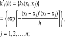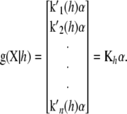
the n × n symmetric matrix of kernels, which can be interpreted as a correlation matrix; and the n × 1 column vector , j = 1, 2, …, n. Then, the minimizing function (6) can be expressed in vectorial manner as the linear function of :

(7)

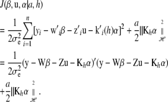
These results can now be employed in (5), leading to a function having , and as arguments, given a and h. One obtains

(8)

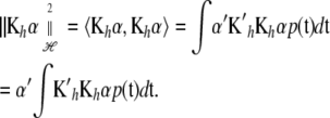
Using (A1) in the appendix,

(9)

Now, a vectorial generalization of the result in (A4) of the appendix is

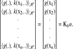This can be used in (9), because the integral is a vector valued inner product of the kernel and of each minimizer (7); that is,

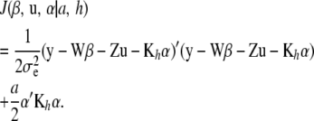
Finally, this can be employed in (8), producing

(10)

Note that (10) does not include a penalty for the random vector u. This is added later on.

Minimizer of the penalized sum of squares:

The gradients of with respect to the parametric and nonparametric coefficients are

and

Noting that K_h is symmetric (so that ; the notation is retained to facilitate analogies with mixed-model methodology), the first-order condition is satisfied by the system

(11)

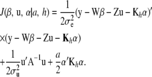
with the notation emphasizing the dependence of the solutions on a and h. There is no unique solution to this system, because the number of equations (p + q + n) exceeds the rank of the coefficient matrix. This problem is solved by a random-effects treatment of u via the assumption , stated earlier. Under this assumption and the penalized-likelihood framework, the objective function to minimize becomes

(12)

Taking derivatives as before, setting to zero and rearranging produces now

(13)

which has full rank if the elements of are defined uniquely, i.e., as a set of linearly independent estimable functions. There is a clear parallel between the forms of the u-equations and of the α-equations. In particular, in the nonparametric part, plays the role of . Hence, one can arrive at representation (12) by making the assumption , where is the “variance” of the -effects, and is their correlation matrix. Fortunately, this inverse is not needed for solving (13) as K_h is a dense n × n matrix. The α-equations can be rearranged such that the solution for the nonparametric coefficients is

Large linear systems such as (13) have been solved routinely in animal breeding since the 1980s (e.g., Quaas and Pollak 1980). System (13) differs from Equation 26 in Gianola et al. (2006), which has instead of . The latter is the correct RKHS representation.

DUAL FORMULATION

The linear model:

The preceding results imply that the RKHS approach is equivalent (this is referred to as a “dual” formulation) to the linear model

(14)

under the assumptions that is a “fixed” vector and that the random effects , and e are distributed independently as , and , respectively. Hence, given h, implementation of the RKHS regression is as in a standard mixed-effects linear model, especially if the kernel matrix does not involve any parameter(s) h. For instance, variance components can be estimated via restricted maximum likelihood; subsequently, point estimates of , and are obtained by solving (13) evaluated at the variance-components estimates. If is large (implying that a is large), the estimated -coefficients are expected to be near 0. A remarkable aspect of the RKHS procedure is the mutual exchange of information between α-coefficients due to the nontrivial correlation structure induced by K_h. This is similar to the exchange of information between relatives induced by A in the classical additive genetic model.

Effective number of parameters:

In a standard regression model (-coefficients only) the degrees of freedom of the model are given by , provided the incidence matrix has full-column rank (this can be assumed without loss of generality). The fitted value is , and the n × n matrix is called the smoother operator (Hastie and Tibshirani 1990). Note that the degrees of freedom can also be arrived at by taking .

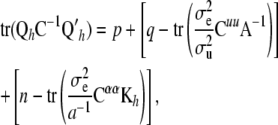
Let now so that in the context of (14), the vector of fitted values is , where C is the coefficient matrix in (13). Hence, a measure of the effective number of parameters fitted in RKHS regression

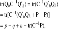where

Further,

(15)

where C^uu and C^αα are the u- and α-blocks of C⁻¹. Then, in some sense is the effective number of additive genetic effects fitted and is the effective number of α-coefficients. If in (12) and a = 0 (equivalently, = ∞), (15) is equal to p + q + n and, in the limit, the degrees of freedom of the model are given by the rank of , so that the model interpolates the data. On the other hand, as and tend to 0 (), the effective number of parameters fitted decreases, and the model becomes less capable of reflecting potentially existing patterns in the data.

Uncertainty about predictions:

Given h and ignoring the error of estimation of variance components, an estimator of the variance–covariance matrix of the estimates of , and of the prediction errors of u and , is given by

Let S_h = Q_hC⁻¹ be the smoothing matrix. The variance–covariance matrix of the vector of fitted values is

and the variance–covariance matrix of the fitted residuals is

In a genetic context, a relevant prediction problem is that of inferring a vector of future observations y* in individuals possessing marker genotypes X*, so that the unknown molecularly marked genetic value, or contribution to phenotype, is . The model for the future observations is

with its coefficients inferred from currently available data y. The point predictor is , and the prediction error variance–covariance matrix is

where I* is an identity matrix with as many rows and columns as there are elements in y*. A confidence band for the elements of y* based on the pointwise standard errors of prediction (Hastie and Tibshirani 1990) is given by , where denotes a vector whose elements are equal to twice the square root of the diagonal elements of . The confidence band does not consider the uncertainty in the estimates of variance components as well as that associated with h.

Tuning parameter:

If the kernel matrix involves one or more h's, some value(s) needs to be arrived at. Typically, cross-validation (CV) is used (e.g., Craven and Wahba 1979; Wahba 1990; Golub et al. 1999). The simplest method (albeit computationally intensive) is the leave-one-out cross-validation measure

where is a vector of fitted values resulting from n fits obtained from deleting y₁, y₂, … , y_n, respectively. For instance, is the fitted value of observation 1 using all data other than y₁, and so on. The value of h chosen results from minimizing over a grid. Clearly, this is not computationally feasible in most quantitative genetic data sets, where n can range from hundreds to millions of observations. In such a situation, one may wish to carry out a cross-validation involving a less intensive level of folding, e.g., a leave 20%-out assessment. A more appealing (and, on some grounds, theoretically firmer) criterion is the generalized cross-validation

Using (15), the statistic becomes

The main difficulty here is the calculation of the inverse matrices under the trace operator. These traces may be approximated (animal breeders have proposed approximations required for REML computations) or estimated via Monte Carlo sampling; e.g., in some Bayesian contexts the diagonal elements of C^uu and C^αα are proportional to posterior variances.

RKHS CHROMOSOME MIXED MODEL

The linear model:

Consider again the additive chromosome specification (3), but now in the context of linear model (14). For ease of presentation, let the number of pairs of chromosomes be C = 2; generalization is straightforward. The unknown function of SNP genotypes to be inferred is

(16)

Using the dual formulation, the model can be written as

(17)

where is an n × n matrix with typical element , is also n × n with typical element and h₂ are the decay parameters corresponding to SNPs in chromosome pairs 1 and 2, respectively, and and are each n × 1 vectors of coefficients. As before, x_i1 and x_i2 are p₁ × 1 and p₂ × 1 genotype incidence vectors pertaining to the appropriate chromosomes; recall that the number of markers in the two chromosomes is given by and , because two dummy variates are needed for coding the three genotypes uniquely. The counterpart of objective function (12) is

(18)

Using the dual formulation, the form of the penalty is equivalent to making the assumption

that is, and are independently and normally distributed with covariance matrices , i = 1, 2. Letting , , the counterpart of (13) is

(19)

where , etc., denote that the solution vector in question depends on .

Implementation:

The procedure can be carried out in a non-Bayesian manner as follows:

• Define a grid of h₁, h₂ values.

• For each point in the grid, estimate , and and (19).

• For each point in the grid, calculate the fitted values

  

  the smoothing matrix , and the generalized cross-validation criterion.

• Choose the combination of h₁, h₂ values optimizing , and predict future observations as outlined previously.

Bayesian approach:

The procedures described for the “global” and chromosome models (14) and (17), respectively, do not take into account uncertainty about unknown parameters. This can be addressed by adopting a Bayesian perspective; see Mallick et al. (2005) and Gianola et al. (2006). Here, a Bayesian analysis of the chromosome model (16) using the dual formulation (17) is outlined.

Let the collection of unknowns be , where, as before, y* is a vector of future phenotypic values to be predicted and

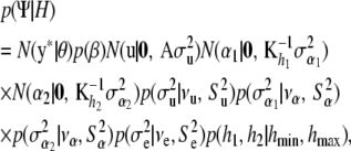
Assume the joint prior density has the form

(20)

where H denotes all hyperparameters (whose values are fixed a priori) and indicates a multivariate normal distribution with appropriate mean vector and covariance matrix; the prior is discussed below. The four variance components are assigned independent scaled inverse chi-square prior distributions with degrees of freedom ν and scale parameters S², with appropriate subscripts. Assign an improper prior distribution to each of the elements of and, as in Mallick et al. (2005), adopt independent uniform priors for h₁ and h₂ with lower and upper boundaries h_min and h_max, respectively.

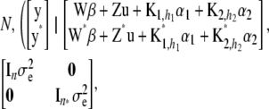
Given , observations are assumed to be conditionally independent, so the distribution of the observed (y) and future (y*) data is

(21)

where n* is the order of the future data vector. Given , and , future observations are independent of past ones. Let and .

Given h₁, h₂ the setting is that of a Bayesian analysis of a mixed linear model, and Markov chain Monte Carlo procedures for this situation are well known (e.g., Wang et al. 1993, 1994; Sorensen and Gianola 2002). All conditional posterior distributions are known, except those of h₁, h₂. A Gibbs–Metropolis sampling scheme can be used in which conditional distributions are used for drawing , and y*, and a Metropolis–Hastings update is employed for h₁ and h₂. The distributions to be sampled from are considered successively.

• Draw location effects from a multivariate normal distribution with mean vector

  (22)

  and covariance matrix .
• Sample additive genetic effects from a normal distribution centered at

  (23)

  and with covariance matrix .
• The conditional posterior distributions of each of the coefficients are multivariate normal as well, with mean vectors

  (24)

  (25)

  and variance–covariance matrices

  (26)

  and

  (27)
• The variance components have scaled inverse chi-square conditional posterior distributions and are conditionally independent. The conditional posterior distributions to sample from are as follows, where ELSE denotes all parameters other than those being sampled,

  (28)

  (29)

  (30)

  and

  (31)

  where is the vector of residuals evaluated at the current sample values of the location effects.
• The most difficult parameters to sample are h₁ and h₂. However, if the kernels do not involve h's this step is omitted from the sampling process. If uniform (bounded) priors are adopted, their conditional posterior density is

  (32)

  where is an indicator function taking the value 1 if both h parameters are between the bounds and 0 otherwise. Further, the residual vector has as its ith element

  

  recalling that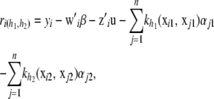

  

  and

  

  Density (32) is not in a recognizable form. However, a Metropolis algorithm (Metropolis et al. 1953), as suggested by Mallick et al. (2005) and Gianola et al. (2006), can be tailored for obtaining samples from the distribution . Let the Markov chain be at state and draw proposal values and from some symmetric candidate-generating distribution. The proposed values are accepted with probability

  

  If the proposal is accepted, then set otherwise, the chain stays at .
• Finally, the vector of yet to be observed phenotypes is inferred from samples drawn from the conditional distribution

  (33)

  with the values of , and h₂ evaluated at the corresponding realizations from the current round of Markov chain Monte Carlo sampling. When the algorithm converges to the equilibrium distribution, the samples of y* drawn are from the predictive distribution , which fully takes into account the uncertainty about all unknown model parameters.

DISCUSSION AND EXTENSIONS

This article presents a procedure for quantitative genetic analysis using information on whole-genome markers, such as SNPs, and phenotypic measurements for some complex candidate trait. Focus is on theory and methods based on RKHS regression, arguably the state of the art in functional data analysis (Wahba 1990; Gu 2002; Wood 2006). The model contains a parametric component, represented by the classical additive genetic model of quantitative genetics, and an unknown function or set of functions of SNP genotypes that is dealt with nonparametrically, as in the generalized additive models of Hastie and Tibshirani (1990). The number of nonparametric functions employed is a model choice issue, and many alternative specifications can be formulated. Here, a global function was considered, expected to reflect all relevant “genetic signals,” e.g., dominance and various forms of epistasis, as well as a sum of chromosome-specific functions, each of which is expected to capture dominance as well as epistasis involving linked loci at the corresponding chromosome.

The parametric component includes additive genetic effects only. Dominance and (some) epistatic effects can be handled parametrically. However, a standard treatment requires constructing and inverting large and possibly dense matrices such as, e.g., A # A # D # D if an additive × additive × dominance × dominance variance component were to enter into the parameterization; # denotes Hadamard product. Further, the Cockerham–Kempthorne decomposition machinery available for dealing with epistatic variance collapses under inbreeding and selection; e.g., all sorts of covariances between genetic effects crop up, rendering the parametric approach invalid. A related point is related to limitations of the orthodox view of nonadditive genetic effects in quantitative genetics. The classical definitions of epistatis pertain to a model in which effects enter linearly when forming the genotype. However, one could argue that biology is far from linear. For instance, it may not be enlightening to think in terms of variance components in situations in which a phenotype results from a sum of sine and cosine waves or when nonadditivity enters via terms such as , where the a's are effects of alleles at some different loci.

Gianola et al. (2006) discuss how a “nonparametric analog of breeding value” can be derived via a Taylor series expansion; this may have merit in genomic selection contexts in which the objective is to increase (or decrease) additive genetic value for some quantitative trait. Caveats and generalizations of the procedures are discussed next.

Filtering SNPs:

Availability of a massive number of SNPs does not necessarily imply that all markers should be included in a prediction model. Apart from standard preprocessing based on minimum allele frequency or information content, it may well be that predictive ability is enhanced by reducing the dimension of the features used as input in a model. For example, Long et al. (2007) described a machine-learning technique based on filtering (using entropy reduction) and wrapping (Bayesian classification performance), to process >5000 SNPs genotyped in broiler families. Predictive ability of bird mortality was increased when the top (based on information gain) 50 SNPs were downsized to 24. More research is needed in regard to the strategic use of markers, e.g., using a few ones vs. all, or on the assignment of different window-width parameters to genomic regions in a whole-genome treatment.

Model choice:

A natural question is that of the model to be used for predicting phenotypes. For instance, should a chromosome model be adopted, instead of a global specification? Comparison of models is a complex issue, as some specifications are better for describing observed data, while others may have a superior predictive ability. See Sorensen and Waagepetersen (2003) for a case study using several criteria for Bayesian model comparison. Some non-Bayesian techniques are discussed by Hastie and Tibshirani (1990) and Wood (2006). The latter include likelihood ratios evaluated at the penalized likelihood estimates and differences in deviances using approximations to the model degrees of freedom; none takes into account the uncertainty associated with the estimates of the smoothing parameters. A different approach, called BRUTO (Hastie and Tibshirani 1990) is based on iterative minimization of a modification of the generalized cross-validation statistic GCV(.) discussed earlier. For example, in a model with additive functions for each of C chromosomes, there would be 2C tuning parameters involved in the BRUTO iteration. Bayesian methods of model comparison have a stronger formal justification.

Incomplete genotyping:

In animal breeding, it is not feasible to genotype all individuals for the SNPs. For instance, poultry breeding and cattle artificial insemination companies typically genotype sires only. The number of animals with phenotypic information can be in the order of hundreds of thousands, and genotyping is selective, so animals with SNPs are not a random sample from the population. Methods for dealing with incomplete molecular information are discussed by Gianola et al. (2006), and some include sampling of genotypes. Here, the problem is revisited in the light of RKHS regression, primarily to illustrate difficulties.

Assume a global model with a single h parameter. The vector of phenotypic values is partitioned as , where y₁ (n₁ × 1) consists of records of individuals lacking SNP data, and y₂ (n₂ × 1) includes phenotypic data of genotyped individuals. In animal breeding n₁ > p > > n₂. Write the model

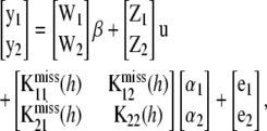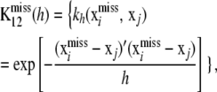
where is an unobserved n₁ × n₁ matrix of kernels, is also an unobserved n₁ × n₂ matrix, is the n₂ × n₂ matrix of observed kernels, and and are n₁ × 1 and n₂ × 1 vectors of coefficients. Specifically

where denotes the vector of unobserved SNP genotypes in individuals with phenotypes y₁. Assign the multivariate normal distribution (suppressing dependence on h in the notation)

where . Given , h, , , , and the phenotypes y₁ and y₂, the best linear unbiased predictor (conditional posterior mean) of u and is the solution to

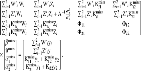(34)

where

As shown in (34) both the coefficient matrix and the vector of right-hand sides depend on . From a Bayesian perspective under Gaussian assumptions,

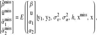where x^miss is the collection of unobserved SNPs and x denotes the SNPs of all genotyped individuals. Assuming , , and h are known, for simplicity, one is interested in arriving at the unconditional expectation

(35)

so the Bayesian solution requires averaging over the conditional distribution . This is a formidable probabilistic imputation, although some simplification is possible. It would seem reasonable to approximate this distribution by , arguing that, conditionally on x, phenotypic values do not provide much additional information about SNP genotypes. Subsequently, form the Bayesian classifier

where is the prior probability of observing genotype configuration in the population. The prior probability can be estimated using models with various degrees of refinement; e.g., one can assume linkage equilibrium and estimate the joint prior probability from the product of the marginal distributions at individual SNP loci. Likewise, can be approximated by some naïve probability calculation, e.g., assuming independence between individuals and loci. The denominator can also be approximated as

where S is a set of missing values having relatively high plausibility. Naïve Bayesian classifiers have been enormously successful in the machine-learning literature (e.g., Elkan 1997) and may prove to be competitive against some involved genotype sampling procedures that have been suggested (Van Arendonk et al. 1989; Fernando et al. 1993; Sheehan and Thomas 1993; Jensen et al. 1995; Kerr and Kinghorn 1996; Jensen and Kong 1999; Fernández et al. 2002; Stricker et al. 2002). Once an approximation to is arrived at, this can be used as mixing distribution in (35). Alternatives are discussed in Gianola et al. (2006), including fitting a bivariate model.

Choice of kernel and discreteness of genotypes:

Following Hastie and Tibshirani (1990) and Wood (2006), the developments carry when the distribution of y is a member of the exponential family. As in density estimation, many candidate kernels are available, and attaining a good predictive behavior is critically dependent on the choice of kernel. As noted, some kernels do not involve tuning parameters; for instance, see González-Recio et al. (2008).

The theory of RKHS regression holds for a continuously valued x. It is unknown if the procedures are robust with respect to using a Gaussian kernel function when, in fact, SNP genotypes or haplotypes are discrete. Silverman (1986) discussed univariate density estimation and concluded that various kernels differed little in mean squared error. It is unknown if this robustness argument holds for RKHS regression (clearly the inner product arguments are valid for the continuous case), but a discrete approximation may work.

A kernel suitable for discrete covariates is proposed here. For a biallelic SNP, there are three possible genotypes at each “locus.” Suppose the elements of x are coded as 0, 1, 2, to denote the appropriate genotypes. For an x vector with p coordinates, its statistical distribution is given by the probabilities of each of the 3^p outcomes. With SNPs, p can be very large (possibly much larger than n), so it is hopeless to estimate the probability distribution of genotypes accurately from observed relative frequencies, and smoothing is required (Silverman 1986). The number of disagreements between a focal x and the observed x_i in subject i is given by

where takes values between 0 and 4p. As an illustration, if “genotype” AABbccDd is the focal point and individual i in the sample is aaBbccDD, then, . Following Silverman (1986), one could use the “binomial” kernel

with ; alternative forms of the kernel function are discussed by Aitchison and Aitken (1976) and Racine and Li (2004). The (pseudo-)RKHS dual formulation would take the form

Alternatively, incidence of the three genotypes at a locus can be described with two “free” dummy variates, as in standard ANOVA. There are p predictor variates, where p/2 is the number of markers. Let x_1k and x_2k be the two dummy variates at locus k (). Define

which give the number of disagreements between a focal and the observed in subject i. Each of the d's varies between 0 and 1. Then, let

each varying between 0 and p/2. Subsequently, consider the “trinomial” kernel

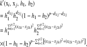where x_i is the “focal” p × 1 vector of covariates and x_j is the observed value in individual j. If each of the h₁, h₂ parameters takes values in 0–1, such that 0 < h₁ + h₂ < 1, then k takes values in 0–1 and is a suitable candidate as kernel, because the matrix would be positive definite. The dual (pseudo-)RKHS representation would be

Then, procedures for inferring the variance components and h parameters outlined in this article would be followed. Research is needed for assessing the adequacy of these approximations. González-Recio et al. (2008) present an application of the trinomial kernel.

Conclusion:

The methods presented here take the whole-genome view of those of Meuwissen et al. (2001), Gianola et al. (2003), Xu (2003), Yi et al. (2003), Ter Braak et al. (2005), Wang et al. (2005), and Zhang and Xu (2005). The main difference is the attempt to capture unknown forms of interaction between many loci that, arguably, parametric models are not able to explore properly, due to either violation of assumptions (for decomposition of epistatic variance) or inadequate statistical machinery for understanding high-level “physiological epistasis.”

An application of the theory presented here is in González-Recio et al. (2008). Using mortality rates observed in 200 families of paternal half-sib broilers, these authors compared the predictive ability of a standard parametric mixed model against that from linear regression (fitting additive effects of 24 SNPs), kernel regression, RKHS, and the Bayesian regression model of Xu (2003). For RHKS, the kernel consisted of a similarity score between any two SNP sequences. The five models were contrasted in terms of a fivefold predictive cross-validation. Results indicated an advantage of RKHS, which had a global “accuracy” that was twice as large as the one from the mixed model, was 2.5 times larger than the one attained with the linear regression specification, and exceeded that attained with the procedure of Xu (2003) by 25%. However, predictive cross-validation accuracy was not large, probably due to the very low heritability of the trait used for the case study, chick mortality.

It should be noted that a kernel function explores commonalities in some sense; e.g., in a chromosome model markers in a contiguous position borrow information. In spirit, this is similar to the use of relationship or identity-by-descent matrices between individuals or cultivars in animal and plant breeding, respectively.

Recent developments in nonparametric statistics and machine learning offer exciting avenues for whole-genome analysis of quantitative traits and perhaps suggest a change in analytical paradigms. This theoretical article intends to make a contribution in this direction.

APPENDIX

In an Euclidean space of dimension n, the dot product between vectors v and w is , and the norm is . The inner product generalizes the dot product to vectors of infinite dimension. For instance, in a vector space of real functions with domain , the inner product is

and the norm is . If x is a continuous random variable with probability density function , the inner product (Hastie and Tibshirani 1990) is

(A1)

Consider now the choice of basis functions for x, that is, a transformation of the input (SNP) space to be used as regressors in the nonparametric regression. A kernel is a function that maps inputs α, x into some space, and the kernel is said to be symmetric if (Rasmussen and Williams 2006). A kernel involving random vectors x, t is positive definite if

for all functions g, where is a joint density. An eigenfunction of positive-definite kernel k with eigenvalue λ satisfies the equation

There are an infinite number of eigenfunctions with an ordering corresponding to λ₁ ≥ λ₂ …. The eigenfunctions are orthogonal and can be normalized to satisfy

(A2)

Mercer's theorem (Rasmussen and Williams 2006) enables expressing a kernel in terms of its eigendecomposition such that

(A3)

If all eigenvalues are positive, the sum is infinite. If, on the other hand, the sum terminates at some value p, say, this yields a degenerate kernel of rank p. For example, in a linear random-regression model with coefficients in which the x variables are transformed into orthonormal basis functions , the regression function evaluated at points x₁, x₂, … , x_n generates the covariance matrix of rank n; recall that, in our situation, n < < p. Here, the eigendecomposition becomes that of a covariance matrix of finite dimension. In general, is called a covariance function, and K is an infinite-dimensional generalization of a covariance matrix. The kernel is clearly symmetric, as .

The notation and will denote that, at some fixed point x*, these functions take values and , respectively. A space of functions ℋ is a RKHS with kernel k if the two following conditions are met (Wahba 2002; Mallick et al. 2005; Rasmussen and Williams 2006):

• For every x, is in the Hilbert space ℋ.

• For all x and for every g in ℋ the inner product holds; this is a reproducing property, in some sense.

Consider now a Hilbert space constituted by linear combinations of the orthonormal eigenfunctions; e.g., and , where f_i and v_i are loadings or regression coefficients on the eigenfunctions. Using definition (A1) and orthonormality condition (A2), the inner product is

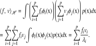Because , the Hilbert space has a norm. In its infinite-dimensional form , this implies that the sequence of f_i coefficients must decay quickly, which imposes smoothness conditions (Rasmussen and Williams 2006).

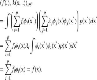
Next, examine if is in the Hilbert space spanned by functions such as f and v above. First, recall the eigendecomposition of kernel . Using again the orthogonality property, the inner product

(A4)

This shows that the inner product between the function and the kernel reproduces the function. Also

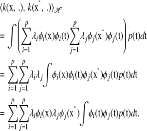Because the eigenfunctions are orthogonal, terms where i ≠ j vanish, and recall from (A2) that , so

(A5)

Hence, the inner product of kernels produces kernel . This demonstrates that the Hilbert space constituted by linear combinations of the eigenfunctions of k has the reproducing kernel properties.

References

- Aitchison, J., and C. G. G. Aitken, 1976. Multivariate binary discrimination by the kernel method. Biometrika 63 413–420. [Google Scholar]
- Aronszajn, N., 1950. Theory of reproducing kernels. Trans. Am. Math. Soc. 68 337–404. [Google Scholar]
- Balding, D. J., 2006. A tutorial on statistical methods for population association studies. Nat. Rev. Genet. 7 781–791. [DOI] [PubMed] [Google Scholar]
- Chang, H. L. A., 1988. Studies on estimation of genetic variances under nonadditive gene action. Ph.D. Thesis, University of Illinois, Urbana-Champaign, IL.
- Cheverud, J. M., and E. J. Routman, 1995. Epistasis and its contribution to genetic variance components. Genetics 139 1455–1461. [DOI] [PMC free article] [PubMed] [Google Scholar]
- Cockerham, C. C., 1954. An extension of the concept of partitioning hereditary variance for analysis of covariances among relatives when epistasis is present. Genetics 39 859–882. [DOI] [PMC free article] [PubMed] [Google Scholar]
- Craven, P., and G. Wahba, 1979. Smoothing noisy data with spline functions. Num. Math. 31 377–403. [Google Scholar]
- Dekkers, J. C. M., and F. Hospital, 2002. The use of molecular genetics in the improvement of agricultural populations. Nat. Rev. Genet. 3 22–32. [DOI] [PubMed] [Google Scholar]
- Elkan, C., 1997. Boosting and naïve Bayesian learning. Technical Report. University of California, San Diego.
- Fenster, C. B., and L. F. Galloway, 2000. Population differentiation in an annual legume: genetic architecture. Evolution 54 1157–1172. [DOI] [PubMed] [Google Scholar]
- Fernández, S. A., R. L. Fernando, B. Gulbrandtsen, C. Stricker, M. Schelling et al., 2002. Irreducibility and efficiency of ESIP to sample marker genotypes in large pedigrees with loops. Genet. Sel. Evol. 34 537–555. [DOI] [PMC free article] [PubMed] [Google Scholar]
- Fernando, R. L., and M. Grossman, 1989. Marker assisted selection using best linear unbiased prediction. Genet. Sel. Evol. 21 467–477. [Google Scholar]
- Fernando, R. L., C. Stricker and R. C. Elston, 1993. An efficient algorithm to compute the posterior genotypic distribution for every member of a pedigree without loops. Theor. Appl. Genet. 87 89–93. [DOI] [PubMed] [Google Scholar]
- Fox, J., 2005. Introduction to nonparametric regression. Lecture Notes. http://socserv.mcmaster.ca/jfox/Courses/Oxford.
- Franklin, I., and R. C. Lewontin, 1970. Is the gene the unit of selection? Genetics 65 707–734. [DOI] [PMC free article] [PubMed] [Google Scholar]
- Gianola, D., M. Perez-Enciso and M. A. Toro, 2003. On marker-assisted prediction of genetic value: beyond the ridge. Genetics 163 347–365. [DOI] [PMC free article] [PubMed] [Google Scholar]
- Gianola, D., R. L. Fernando and A. Stella, 2006. Genomic assisted prediction of genetic value with semi-parametric procedures. Genetics 173 1761–1776. [DOI] [PMC free article] [PubMed] [Google Scholar]
- Golub, T. R., D. Slonim, P. Tamayo, C. Huard, M. Gasenbeek et al., 1999. Molecular classification of cancer: class discovery and class prediction by gene expression monitoring. Science 286 531–537. [DOI] [PubMed] [Google Scholar]
- González-Recio, O., D. Gianola, N. Long, K. A. Weigel, G. J. M. Rosa et al., 2008. Non-parametric methods for incorporating genomic information into genetic evaluations: an application to mortality in broilers. Genetics 178 2305–2313. [DOI] [PMC free article] [PubMed] [Google Scholar]
- Gu, C., 2002. Smoothing Spline ANOVA Models. Springer, New York.
- Hartl, D. L., and E. W. Jones, 2005. Genetics: Analysis of Genes and Genomes, Ed. 6. Jones & Bartlett, Boston.
- Hastie, T. J., and R. J. Tibshirani, 1990. Generalized Additive Models. Chapman & Hall, London.
- Hayes, B., J. Laerdahl, D. Lien, A. Adzhubei and B. Høyheim, 2004. Large scale discovery of single nucleotide polymorphism (SNP) markers in Atlantic Salmon (Salmo salar). AKVAFORSK, Institute of Aquaculture Research, Aas, Norway. www.mabit.no/pdf/hayes.pdf.
- Hoeting, J. A., D. Madigan, A. E. Raftery and C. T. Volinsky, 1999. Bayesian model averaging: a tutorial. Stat. Sci. 14 382–417. [Google Scholar]
- Jensen, C. S., and A. Kong, 1999. Blocking Gibbs sampling for linkage analysis in large pedigrees with many loops. Am. J. Hum. Genet. 65 885–901. [DOI] [PMC free article] [PubMed] [Google Scholar]
- Jensen, C. S., A. Kong and U. Kjaerulff, 1995. Blocking Gibbs sampling in very large probabilistic expert systems. Int. J. Hum. Comp. Stud. 42 647–666. [Google Scholar]
- Kempthorne, O., 1954. The correlation between relatives in a random mating population. Proc. R. Soc. Lond. Ser. B 143 103–113. [PubMed] [Google Scholar]
- Kerr, R. J., and B. P. Kinghorn, 1996. An efficient algorithm for segregation analysis in large populations. J. Anim. Breed. Genet. 113 457–469. [Google Scholar]
- Kimeldorf, G., and G. Wahba, 1971. Some results on Tchebycheffian spline functions. J. Math. Anal. Appl. 33 82–95. [Google Scholar]
- Kimura, M., 1965. Attainment of quasi-linkage equilibrium when gene frequencies are changing. Genetics 52 875–890. [DOI] [PMC free article] [PubMed] [Google Scholar]
- Long, N., D. Gianola, G. J. M. Rosa, K. Weigel and S. Avendaño, 2007. Machine learning classification procedure for selecting SNPs in genomic selection: application to early mortality in broilers. J. Anim. Breed. Genet. 124 377–389. [DOI] [PubMed] [Google Scholar]
- Mallick, B. K., D. Ghosh and M. Ghosh, 2005. Bayesian classification of tumours by using gene expression data. J. R. Stat. Soc. B 67 219–234. [Google Scholar]
- Metropolis, N., A. W. Rosenbluth, M. N. Rosenbluth, A. H. Teller and E. Teller, 1953. Equations of state calculations by fast computing machines. J. Chem. Phys. 21 1087–1091. [Google Scholar]
- Meuwissen, T. H. E., B. J. Hayes and M. E. Goddard, 2001. Is it possible to predict the total genetic merit under a very dense marker map? Genetics 157 1819–1829. [DOI] [PMC free article] [PubMed] [Google Scholar]
- O'Sullivan, F., B. S. Yandell and W. J. Raynor, 1986. Automatic smoothing of regression functions in generalized linear models. J. Am. Stat. Assoc. 81 96–103. [Google Scholar]
- Quaas, R. L., and E. J. Pollak, 1980. Mixed model methodology for farm and ranch beef cattle testing programs. J. Anim. Sci. 51 1277–1287. [Google Scholar]
- Racine, J., and Q. Li, 2004. Nonparametric estimation of regression functions with both categorical and continuous data. J. Econometrics 119 99–130. [Google Scholar]
- Rasmussen, C. E., and C. K. I. Williams, 2006. Gaussian Processes for Machine Learning. MIT Press, Cambridge, MA.
- Sheehan, N., and A. Thomas, 1993. On the irreducibility of a Markov chain defined on a space of genotype configurations by a sample scheme. Biometrics 49 163–175. [PubMed] [Google Scholar]
- Silverman, B. W., 1986. Density Estimation for Statistics and Data Analysis. Chapman & Hall, London.
- Soller, M., and J. Beckmann, 1982. Restriction fragment length polymorphisms and genetic improvement, pp. 396–404 in Proceedings of the 2nd World Congress on Genetics Applied to Livestock Production, Vol. 6. Editorial Garsi, Madrid.
- Sorensen, D., and D. Gianola, 2002. Likelihood, Bayesian, and MCMC Methods in Quantitative Genetics. Springer-Verlag, New York.
- Sorensen, D., and R. Waagepetersen, 2003. Normal linear models with genetically structured residual variance heterogeneity: a case study. Genet. Res. 82 207–222. [DOI] [PubMed] [Google Scholar]
- Stricker, C., M. Schelling, F. Du, I. Hoeschele, S. A. Fernandez et al., 2002. A comparison of efficient genotype samplers for complex pedigrees and multiple linked loci. Proceedings of 7th World Congress on Genetics Applied to Livestock Production, INRA, Castanet-Tolosan, France, CD-ROM Communication no. 21–12.
- Takezawa, K., 2005. Introduction to Non-Parametric Regression. Wiley-Interscience, Hoboken, NJ.
- Ter Braak, C. J. F., M. Boer and M. Bink, 2005 Extending Xu's (2003) Bayesian model for estimating polygenic effects using markers of the entire genome. Genetics 170 1435–1438. [DOI] [PMC free article] [PubMed] [Google Scholar]
- Van Arendonk, J. A. M., C. Smith and B. W. Kennedy, 1989. Method to estimate genotype probabilities at individual loci in farm livestock. Theor. Appl. Genet. 78 735–740. [DOI] [PubMed] [Google Scholar]
- Wahba, G., 1990. Spline Models for Observational Data. Society for Industrial and Applied Mathematics, Philadelphia.
- Wahba, G., 1999. Support vector machines, reproducing kernel Hilbert spaces and the randomized GAVC, pp. 68–88 in Advances in Kernel Methods, edited by B. Schölkopf, C. Burges and A. Smola. MIT Press, Cambridge, MA.
- Wahba, G., 2002. Soft and hard classification by reproducing kernel Hilbert spaces methods. Proc. Natl. Acad. Sci. USA 99 16524–16530. [DOI] [PMC free article] [PubMed] [Google Scholar]
- Wang, C. S., J. J. Rutledge and D. Gianola, 1993. Marginal inferences about variance components in a mixed linear model using Gibbs sampling. Genet. Sel. Evol. 25 41–62. [Google Scholar]
- Wang, C. S., J. J. Rutledge and D. Gianola, 1994. Bayesian analysis of mixed linear models via Gibbs sampling with an application to litter size in Iberian pigs. Genet. Sel. Evol. 26 91–115. [Google Scholar]
- Wang, H., Y. M. Zhang, X. Li, G. Masinde, S. Mohan et al., 2005. Bayesian shrinkage estimation of quantitative trait loci parameters. Genetics 170 465–480. [DOI] [PMC free article] [PubMed] [Google Scholar]
- Wong, G. K., B. Liu, J. Wang, Y. Zhang, X. Yang et al., 2004. A genetic variation map for chicken with 2.8 million single-nucleotide polymorphisms. Nature 432 717–722. [DOI] [PMC free article] [PubMed] [Google Scholar]
- Wood, S. N., 2006. Generalized Additive Models. Chapman & Hall/CRC Press, Boca Raton, FL.
- Xu, S., 2003. Estimating polygenic effects using markers of the entire genome. Genetics 163 789–801. [DOI] [PMC free article] [PubMed] [Google Scholar]
- Yi, N., G. Varghese and D. A. Allison, 2003. Stochastic search variable selection for identifying multiple quantitative trait loci. Genetics 164 1129–1138. [DOI] [PMC free article] [PubMed] [Google Scholar]
- Zhang, Y., and S. Xu, 2005. A penalized maximum-likelihood method for estimating epistatic effects of QTL. Heredity 95 96–104. [DOI] [PubMed] [Google Scholar]