Analyses of circular dichroism spectra of membrane proteins

Abstract

Circular dichroism (CD) spectroscopy is a valuable technique for the determination of protein secondary structures. Many linear and nonlinear algorithms have been developed for the empirical analysis of CD data, using reference databases derived from proteins of known structures. To date, the reference databases used by the various algorithms have all been derived from the spectra of soluble proteins. When applied to the analysis of soluble protein spectra, these methods generally produce calculated secondary structures that correspond well with crystallographic structures. In this study, however, it was shown that when applied to membrane protein spectra, the resulting calculations produce considerably poorer results. One source of this discrepancy may be the altered spectral peak positions (wavelength shifts) of membrane proteins due to the different dielectric of the membrane environment relative to that of water. These results have important consequences for studies that seek to use the existing soluble protein reference databases for the analyses of membrane proteins.

Circular dichroism (CD) spectroscopy is a important technique in structural biology for examining the folding, conformational changes, and especially secondary structures of proteins. Its utility as a quantitative method has been based on empirical methods that use a wide variety of computational algorithms with reference databases composed of spectra of soluble proteins of known (crystallographic) structures. These permit the determination of the secondary structural content of an “unknown” protein (for a review, see Woody 1995). FTIR spectroscopy also has utility for studies of protein secondary structures, although in general it is more demanding in terms of material and/or time for data collection. CD spectroscopy is exhibiting a resurgence in the postgenomic era, especially with the development of synchrotron radiation circular dichroism (SRCD), whose additional information content provides the potential for fold recognition (Wallace and Janes 2001). CD may become particularly important for elucidating the structures of membrane proteins, a class of protein generally bypassed by structural genomics initiatives (Blundell and Mizuguchi 2000).

Over the years a large number of computational algorithms have been developed that permit the calculation of secondary structures of soluble proteins from their CD spectra. The success of a given method on a given protein is related to how representative the components of the reference database are for the spectral and structural characteristics of the protein being probed. To date, the available reference databases have included proteins representing a wide range of structural types (e.g., Chang et al. 1978^; Pancoska and Keiderling 1991^; Johnson 1999^; Sreerama and Woody 2000^; Sreerama et al. 2000); however, they have not included any members of the class of membrane proteins. In principle, these empirical methods should be suitable for analyses of membrane proteins if the spectral characteristics of this class of proteins are well represented in the reference database spectra; however, membrane proteins are embedded in hydrophobic lipid environments instead of the aqueous milieu of soluble proteins. Studies on small proteins and model peptides (Cascio and Wallace 1994, 1995; Chen and Wallace 1997a,b) have indicated that some of the spectral characteristics are dependent on the dielectric constant of the surrounding medium. This is because both the ground and excited state transitions associated with the peptide bond (n → π*, π → π*) can be affected by the solvent polarisability, and thus the energies of the transitions (and, consequently, the resulting positions of the peaks) will change. The purpose of the present study was to examine whether the characteristics of the existing CD reference database components are sufficient to permit accurate analyses of the secondary structures of membrane proteins from their CD spectra. This study has used both membrane proteins with predominantly helical structures and membrane proteins with predominantly β-strand structures, all of whose crystal structures have been determined, as representative test proteins.

Results

Samples and CD measurements

The membrane protein samples were, in general, examined in the solvent/buffer/detergent system from which they had been crystallized, to permit direct comparisons with their secondary structures in the crystal environment, because the conformations of membrane proteins can be sensitive to the environment (especially detergents) present.

SRCD was used to collect the data for all of the samples because many of them were examined in strongly absorbing buffer (and detergent) systems, which can prevent measurement of the CD spectra in conventional CD instruments below ~200 nm. Data only down to this wavelength are not very accurate for analyses of protein secondary structure (Toumadje et al. 1992). However, because the beam in the SRCD is much more intense at the low wavelengths, it permits data collection to much lower wavelengths in the VUV region (Wallace 2000). In all cases in this study, data collection was possible down to at least 171 nm (in many cases, to 160 nm). As a control, two soluble proteins (myoglobin and concanavalin A) and one membrane protein (cytochrome oxidase) in low-absorbing solvents were also examined in a conventional CD instrument. The SRCD spectra were very similar to the CD spectra for each of these proteins, although they differed slightly at the low wavelength extreme of the conventional CD spectra, that is, below ~180 nm (Lees and Wallace 2002). Because the majority of the reference databases did not extend below 185 nm, it made little difference to the results if the CD spectra were used for the analyses instead of the SRCD spectra. Therefore, for consistency, only the results of analyses of SRCD spectra are reported in this article.

Comparisons of spectral characteristics of soluble and membrane proteins

In this study, a number of soluble and membrane proteins were examined by CD spectroscopy. Examples of both mostly helical and mostly β-strand-containing proteins were used to determine if any of the trends observed were correlated with the secondary structure type rather than with the class of protein. In this article, for illustrative purposes, we present pairs of soluble and membrane proteins with relatively similar secondary structural compositions, as determined from their crystal structures (Tables 1a, 1b) to facilitate comparisons of spectral shapes of the helical (Fig. 1 ▶) and β-strand (Fig. 2 ▶) types of proteins. Because soluble and membrane proteins tend to adopt different types of fold motifs, while the pairs shown here have similar secondary structures, they do not have similar folds (although this should not result in any substantial differences in the UV- as opposed to the VUV-region of the spectrum). The helical proteins compared are myoglobin and MscL, and the β-strand proteins are ConA and FepA. However, similar trends were observed for all the proteins examined in this study: That is, roughly similarly shaped curves in the far UV (but not VUV) wavelength range were obtained for all the helical and all the β-strand proteins, respectively. Because the VUV region contains transitions that have been attributed to charge transfer, and may be more reflective of tertiary than secondary structural features, the very low wavelength data are not expected to be similar for proteins with different folds, even if their secondary structures are similar (Wallace and Janes 2001).

Table 1a.

Calculated secondary structures from PDB files (soluble proteins)

Protein:	Mb				ConA
Method	Helix	Sheet	Turn	Other	Helix	Sheet	Turn	Other
DSSP	0.75	0.00	0.11	0.14	0.04	0.46	0.12	0.38
Procheck	0.84	0.00	0.11	0.05	0.08	0.56	0.15	0.22
STRIDE	0.80	0.00	0.10	0.11	0.04	0.48	0.29	0.19
Xtlsstr	0.81	0.00	0.05	0.14	0.04	0.37	0.12	0.47
Promotif	0.75	0.00	0.10	0.15	0.05	0.45	0.31	0.19
Average	0.79	0.00	0.09	0.12	0.05	0.46	0.20	0.29
SD	0.04	0.00	0.02	0.04	0.02	0.07	0.09	0.13

Calculated secondary structures derived from the crystal structure. PDB files using different algorithms for the soluble proteins Mb and ConA. Average values from all the methods and their standard deviations (SD) are also presented.

Table 1b.

Calculated secondary structures from PDB files (membrane proteins)

Protein: Method	Helix	Sheet	Turn	Other	Helix	Sheet	Turn	Other
	MscL				cox
DSSP	0.51	0.00	0.11	0.38	0.42	0.17	0.09	0.32
Procheck	0.57	0.00	0.08	0.35	0.48	0.19	0.10	0.23
STRIDE	0.54	0.00	0.32	0.14	0.42	0.18	0.20	0.20
Xtlsstr	0.48	0.05	0.16	0.31	0.44	0.10	0.10	0.37
Promotif	0.51	0.00	0.39	0.11	0.41	0.18	0.19	0.22
Average	0.52	0.01	0.21	0.26	0.43	0.16	0.14	0.27
SD	0.03	0.02	0.13	0.12	0.03	0.04	0.05	0.07

	cytbc1				BR
DSSP	0.52	0.10	0.10	0.29	0.76	0.05	0.08	0.11
Procheck	0.59	0.12	0.12	0.17	0.83	0.06	0.07	0.04
STRIDE	0.53	0.10	0.20	0.16	0.77	0.05	0.10	0.08
Xtlsstr	0.47	0.05	0.16	0.32	0.76	0.04	0.06	0.14
Promotif	0.51	0.09	0.22	0.18	0.76	0.05	0.09	0.09
Average	0.52	0.09	0.16	0.23	0.78	0.05	0.08	0.09
SD	0.04	0.03	0.05	0.07	0.03	0.01	0.02	0.04

	FepA				FhuA
DSSP	0.06	0.50	0.01	0.43	0.07	0.54	0.10	0.29
Procheck	0.08	0.57	0.13	0.23	0.08	0.61	0.13	0.18
STRIDE	0.06	0.47	0.21	0.26	0.06	0.54	0.25	0.15
Xtlsstr	0.06	0.38	0.12	0.44	0.06	0.36	0.12	0.47
Promotif	0.06	0.52	0.19	0.24	0.06	0.55	0.27	0.13
Average	0.06	0.49	0.13	0.32	0.07	0.52	0.17	0.24
SD	0.01	0.07	0.08	0.11	0.01	0.10	0.08	0.14

	LamB				OmpF
Calculated secondary structures derived from the crystal structure PDB files using different algorithms for the membrane proteins used in this study. Average values from all the methods and their standard deviations (SD) are also presented.
DSSP	0.03	0.61	0.11	0.26	0.04	0.59	0.13	0.23
Procheck	0.04	0.67	0.13	0.16	0.06	0.67	0.16	0.11
STRIDE	0.03	0.62	0.22	0.13	0.06	0.63	0.21	0.11
Xtlsstr	0.04	0.45	0.09	0.42	0.05	0.42	0.14	0.39
Promotif	0.03	0.60	0.22	0.15	0.04	0.58	0.25	0.13
Average	0.03	0.59	0.16	0.23	0.05	0.58	0.18	0.19
SD	0.01	0.08	0.06	0.12	0.01	0.10	0.05	0.12

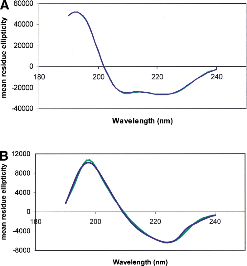
Figure 1.

CD spectra of proteins with high helical contents: Mb (light blue) and MscL (dark blue).

Figure 2.

CD spectra of proteins with high β contents: ConA (light blue) and FepA (dark blue).

For the most part, both the soluble and membrane protein spectra have similar shapes: for predominantly helical structures, negative bands at ~222 and 210 nm, and positive bands at ~192 nm; for β-strands, negative bands at ~215 and 180 nm, and positive bands at ~196 nm. However, the relative magnitudes and positions of the peaks appeared to differ somewhat between the membrane and soluble proteins, even for ones with similar secondary structural contents (Figs. 1 ▶, 2 ▶).

The peak positions for a relatively large number of helical and β-strand soluble proteins were obtained from spectra in the existing CD reference databases as well as from the spectra of proteins measured in this study. By comparison, however, the number of solved membrane protein structures available for study by CD to date is quite small. Hence, any statistically significant quantitation of the extent of the shifts between soluble and membrane proteins is not yet possible with the data presently available, although qualitative trends can be seen. In the examples examined in this study, it appears that for predominately helical membrane proteins, the n → π* and π → π* transitions can be shifted by as much as a few nanometers. The different transitions tend to be shifted to different extents, as had been observed previously for systematic studies of model peptides and small proteins (Wallace et al. 1984; Cascio and Wallace 1994, 1995; Chen and Wallace 1997a,b). The peak positions for soluble β-strand proteins are much more variable than for helical proteins, and this is likely to be a consequence of the variations in the geometries of the various types of β structures (e.g., barrels, sheets, propellers, β-helices, etc.) found in proteins (J.G. Lees and B.A. Wallace, in prep.). The variation in peak positions appears to be less for the four β-strand membrane proteins examined in this study than for the β-strand soluble proteins, but that may simply be due to the fact that all the membrane proteins have had somewhat similar barrel motifs (albeit with different twists and strand numbers) (J.G. Lees and B.A. Wallace, in prep.). Nevertheless, the β-strand membrane protein peaks also appeared to be shifted with respect to the β-strand soluble proteins, in some cases by more than several nanometers.

The CD spectra of membrane proteins have been shown to exhibit absorption flattening and differential scattering artifacts (Wallace and Mao 1984; Teeters et al. 1987; Wallace and Teeters 1987) when the proteins are embedded in large membrane particles. The detector geometries of the SRCD instrument and our modified conventional CD instrument minimize the scattering effects, and under the detergent conditions used in this study, the absorption flattening effects are essentially nonexistent (Mao and Wallace 1984; Wallace and Teeters 1987). Therefore, these are unlikely to be the source of the spectral differences seen between the soluble and membrane proteins. In addition, membrane protein structures in general exhibit φ, ψ angles that obey the normal Ramachandran conventions, so any differences seen in the spectra are also unlikely to arise from true differences in structural features present in the proteins. A primary source of the spectral differences is more likely to be due to the differences in the dielectric constants of the surrounding hydrophobic environment of the membrane proteins and that of the water surrounding the soluble proteins. This notion is supported by the correspondence between the spectra shifts seen for the membrane proteins examined in this study and those seen in the previous systematic studies of shift with solvent dielectric for small peptides and proteins (Chen and Wallace 1997a,b). Alternatively, hydrogen bonding to the aqueous solvent could change the electronic distribution in the amides, and hence, the peak positions and magnitudes.

Secondary structure definitions

Because there are many ways of defining secondary structures (φ, ψ angles, contact distances, hydrogen bonds, etc.), a number of algorithms were used to determine the secondary structures from the protein crystal structures, calculated from their Protein Data Bank (PDB) files. It has been suggested that XtlSSTR (King and Johnson 1999) is the most appropriate method for comparisons with spectroscopic data, but we also included a number of other methods, to examine how much variation there was with method and whether the method of calculation was biasing our conclusions. Tables 1a and 1b include the results obtained for all methods, plus an average of the methods, and their standard deviations. In general, the calculated contents of the highly helical proteins are more consistent than are those for the mostly β-strand proteins. This may be because the geometric parameters for helical secondary structures vary less and helices are better defined and recognized features.

Soluble protein analyses from CD data

The analysis results obtained in this study on the soluble proteins are comparable to other studies comparing these algorithms on soluble proteins (e.g., Johnson 1999^; Sreerama and Woody 2000), and were not meant to replicate the considerable cadre of such studies that have previously been reported. The principal purposes for doing the calculations on the soluble protein data in this study were: (1) to show the quality of the results and the fits are not a consequence of using SRCD rather than CD data, (2) to demonstrate how the wide range of algorithms used in this study behave, and (3) to calculate a consistent parameter (the NRMSD) to quantitate the goodness of fit for all methods.

The secondary structures were calculated from the CD data for Mb and ConA using a wide range of algorithms and reference databases. Reference databases 1, 2, and 5 included data to 178, whereas some databases only included data to 190 nm, and the K2D method used data only to 200 nm. In general, the fits [as assessed by the NRMSD parameter (Table 2a)], the correctness of the results [as assessed by the R parameters (Table 2a)] and a visual inspection of the back-calculated and measured spectra (Fig. 3A,B ▶), are excellent for all methods and databases for Mb, the helical protein, and excellent for some, and reasonably good for most databases for ConA, the β-strand protein. However, in general, considerably poorer results were obtained for all the β-strand proteins than for the helical proteins, consistent with observations in the literature that β-strands are less well determined by all these methods. In general, analyses of β-strand proteins tend to be less accurate, and this is in part due to the lower intensity of the β spectrum, which is dwarfed by the much larger helical spectrum (Pancoska et al. 1992), and, in part, because β-strand structures are more variable than helical ones, thus giving rise to more diverse spectra.

Table 2a.

Calculated NRMSD and R parameters for CD data (soluble proteins)

Protein:		Mb				ConA
Method	db	NRMSD	Rav	RXS	RP	NRMSD	Rav	RXS	RP
Selcon	1	0.073	0.139	0.201	0.06	0.544	0.112	0.210	0.04
	2	0.029	0.068	0.074	0.02	0.265	0.240	0.082	0.12
	3	0.061	0.050	0.034	0.01	0.305	0.068	0.200	0.02
	4	0.045	0.038	0.030	0.00	0.301	0.105	0.179	0.05
	5	0.060	0.145	0.207	0.05	0.515	0.262	0.260	0.14
	6	0.062	0.050	0.034	0.01	0.300	0.061	0.203	0.02
	7	0.046	0.038	0.030	0.00	0.266	0.159	0.155	0.09
Contin	1	0.023	0.130	0.192	0.09	0.087	0.074	0.182	0.04
	2	0.026	0.057	0.119	0.05	0.081	0.218	0.100	0.14
	3	0.019	0.078	0.108	0.04	0.064	0.140	0.138	0.11
	4	0.016	0.047	0.033	0.00	0.049	0.187	0.163	0.10
	5	0.031	0.169	0.231	0.09	0.304	0.277	0.275	0.16
	6	0.016	0.026	0.044	0.00	0.049	0.056	0.236	0.03
	7	0.016	0.038	0.034	0.01	0.049	0.065	0.245	0.04
CDSSTR	1	0.011	0.093	0.155	0.04	0.041	0.136	0.172	0.07
	2	0.011	0.021	0.075	0.02	0.021	0.200	0.064	0.11
	3	0.007	0.157	0.095	0.08	0.026	0.126	0.182	0.06
	4	0.005	0.091	0.085	0.01	0.026	0.216	0.214	0.10
	5	0.021	0.153	0.215	0.08	0.037	0.386	0.384	0.20
	6	0.007	0.157	0.095	0.06	0.031	0.136	0.134	0.09
	7	0.004	0.167	0.105	0.08	0.033	0.286	0.284	0.17
K2D		0.066	0.117	0.055	0.02	0.089	0.254	0.256	0.04
VARSLC		nd	0.103	0.165	0.05	nd	0.250	0.092	0.10
Average		0.030	0.093	0.105	0.04	0.158	0.175	0.192	0.09

db = database number.

nd = not determined.

ns = no solution.

The NRMSD is a fit parameter, which is a measure of the difference between the experimental ellipticities and the ellipticities of the back-calculated spectra for the derived structure. It is defined as Σ[(θexp − θcal)²/(θexp)²]^½, summed over all wavelengths.

The R-values are measures of the correctness of the results, as indicated by the differences between the secondary structure as found in the crystal structure, and the secondary structure calculated from the CD spectrum. They are defined as R = Σ[f_Xray − f_CD], summed over helical, sheet, and turn secondary structure types. R_av uses the average X-ray structure derived from all methods (see Table 1) and R_XS uses the value calculated by the program XtlSSTR. R_P calculates the correctness for only the main type of secondary structure present (i.e., helix or sheet).

The best fits (lowest NRMSD values) are listed in bold, and include all values ≤0.05.

The best results (lowest R values) are listed in bold, and include all values ≤0.1.

Figure 3.

(A) Back-calculated spectrum (blue) for the lowest R_av solution (CDSSTR2) for myoglobin compared with the experimental spectrum (green). (B) Back-calculated spectrum (blue) for the lowest R_av solution (CONTIN6) for ConA compared with the experimental spectrum (green).

The best fits (lowest NRMSDs) tended to correspond with one of the best results (lowest R_av, R_xs, or R_P) (Table 2a). For myoglobin, all the methods/data sets that produced low NRMSD values also gave good results in at least one of the R-value calculations. No R-value was worse than 0.21 (most were under 0.1) and only one NRMSD was greater than 0.07. For ConA, there were only two cases (CDSSTR5 and CDSSTR7) that produced low NRMSD values but for which the R-values were not among the lowest. Most R-values were below 0.2, and a majority of the NRMSDs were below 0.1. The best results (lowest R_av) (Fig. 3A,B ▶) and the best fit (lowest NRMSD) solutions (data not shown) both reproduce the experimental spectra nearly exactly. The best fits and best results were, therefore, highly correlated for both the helical and β-sheet proteins.

One of the reasons the fits of the soluble proteins may not be “perfect” is that the algorithms used in the calculations are very sensitive to the magnitudes of the spectra. Even between databases, the reported spectra of the same protein may differ somewhat in magnitude (Chang et al. 1978; Johnson 1999; Sreerama and Woody 2000). Therefore, the magnitudes of the protein spectra used in this study are based on calculations using quantitative amino acid analyses, and using calibrated values for the sample pathlengths, to ensure consistency between samples.

A concern for these analyses could be that a close homolog of one of the soluble test proteins (horse versus whale Mb) and ConA are both included in a number of the protein databases used for the analyses, and thus might be expected to give biased good results. To mitigate against this, a number of test runs were done with the various programs and databases after removal of the homologous protein. The results obtained were virtually indistinguishable (differed by ~2% or less in any fraction of secondary structure) from those obtained with the sample protein included in the database. This suggests that the results seen here are not a consequence of the inclusion of specific proteins in the spectral databases. We also checked this using several soluble proteins not included in the reference databases (J.G. Lees and B.A. Wallace, data not shown) and obtained comparable results.

The various methods to calculate the secondary structures from the PDB files, while giving somewhat different results for the secondary structural compositions, especially for β-strand proteins, produce roughly comparable results in terms of accuracy of the spectral determinations. Therefore, in this study we made no conclusion as to which is the most appropriate, and we report here the overall R-values calculated in two different ways (Tables 2a, 2b) to demonstrate the conclusions are not affected by the specific defining algorithm used. In addition, because the minor conformational types (turn, polyproline, other) are more variable and less well defined, an R_P value was calculated for each protein, which reflects the accuracy in defining just the principal secondary structural type. Even in relatively poor fits, the calculated values of the principal component are considerably better for both the helical and β-strand test proteins. The average values for the two structural types were 0.04 and 0.09, respectively.

Table 2b.

Calculated NRMSD and R parameters for CD data (membrane proteins)

Protein:		MscL				FepA
Method	db	NRMSD	Rav	Rxs	RP	NRMSD	Rav	Rxs	RP
Selcon	1	0.066	0.525	0.557	0.34	ns	ns	ns	ns
	2	0.045	0.699	0.731	0.48	0.247	0.715	0.599	0.41
	3	0.139	0.478	0.510	0.30	0.193	0.102	0.214	0.00
	4	0.042	0.333	0.383	0.28	0.464	0.167	0.151	0.07
	5	0.119	0.524	0.556	0.36	ns	ns	ns	ns
	6	0.138	0.481	0.513	0.31	0.258	0.105	0.191	0.02
	7	0.050	0.325	0.357	0.27	0.392	0.158	0.180	0.05
Contin	1	0.084	0.633	0.617	0.40	0.531	0.754	0.660	0.33
	2	0.025	0.627	0.659	0.41	0.463	0.868	0.752	0.43
	3	0.053	0.576	0.538	0.34	0.118	0.119	0.203	0.02
	4	0.036	0.595	0.627	0.38	0.112	0.146	0.158	0.06
	5	0.057	0.607	0.639	0.39	0.476	0.816	0.720	0.45
	6	0.036	0.514	0.546	0.36	0.116	0.120	0.160	0.04
	7	0.036	0.476	0.508	0.30	0.112	0.111	0.181	0.03
CDSSTR	1	ns	ns	ns	ns	0.021	0.386	0.292	0.19
	2	ns	ns	ns	ns	0.019	0.758	0.642	0.36
	3	0.002	0.559	0.551	0.36	0.023	0.138	0.198	0.03
	4	0.002	0.579	0.571	0.38	0.019	0.188	0.134	0.09
	5	ns	ns	ns	ns	ns	ns	ns	ns
	6	ns	ns	ns	ns	0.029	0.122	0.238	0.00
	7	ns	ns	ns	ns	0.017	0.188	0.208	0.05
K2D		0.101	0.629	0.661	0.41	0.309	0.174	0.268	0.01
VARSLC		nd	0.479	0.511	0.40	ns	ns	ns	ns
Average		0.061	0.536	0.558	0.36	0.206	0.323	0.324	0.14

Because the different algorithms and reference databases used for the calculations of secondary structures from the CD data all produce roughly comparable results, with some methods providing better fits and others better results on specific proteins, we did not select between the methods or reference databases in this study and report the results from a wide range of algorithms (Tables 2a, 2b), to show the generality of the trends.

Membrane protein analyses from CD data

Because the spectral properties of membrane and soluble proteins appear to be somewhat different, this suggested that analyses of membrane protein samples using spectral reference databases derived from soluble proteins, might not produce accurate results, a result borne out here by comparisons of calculated and actual structures. Two structural types of membrane proteins, ones which had either predominantly helical or predominantly β-strand structures, were used to test the accuracy of the analyses on membrane proteins. This study included four primarily helical membrane proteins (MscL, cox, cytbc₁, and BR) and four primarily β-strand membrane proteins (FepA, FhuA, LamB, and OmpF) (Table 1b). For brevity, only the results for one representative sample from each type (MscL and FepA) are reported in Table 2b, but similar trends were observed for all of the membrane protein samples. In general, both the fits (NRMSDs) and the calculated secondary structures are poor for both types of membrane protein, with the β-strand proteins once again having considerably worse fits than the helical proteins, mirroring the results for the two comparable types of soluble proteins. No clear trend could be found for reference databases that produced the best results or best fits.

For all of the membrane proteins, few methods produce R_av or R_xs values of less than 0.1 (none in the case of MscL and FepA). The average R-values for MscL are roughly five times those of the soluble helical test protein and the average R-values for FepA are nearly twice those of the soluble β-strand test protein. The R-values for a number of the β-strand proteins examined (data not shown) were even worse than for FepA (average R_av values as high as 0.61).

The average fit parameter for MscL is twice as large as that for Mb, and for some of the other helical membrane proteins are as much as four times that of Mb (data not shown). More importantly, the best fits in this case do not correspond to the best (or even good) results, and this lack of correspondence is found for virtually all of the other membrane proteins examined. Consequently, the best result produces a back-calculated spectrum (Fig. 4A ▶) that differs considerably from the experimental spectrum, both in peak shape and in peak positions. For FepA and the other β-strand membrane proteins, the average NRMSDs are higher than for the soluble proteins, with one average as high as 0.39, and the best fits also generally do not correspond to good R_av values (Table 2b). However, for a few combinations of method and database, low NRMSD values do correspond to some of the lower R-values for some of the β proteins. The back-calculated fits for the β proteins are generally even poorer than for the helical membrane proteins (Fig. 4B ▶) and differences in peak positions reflect the observed wavelength shifts in the data.

Figure 4.

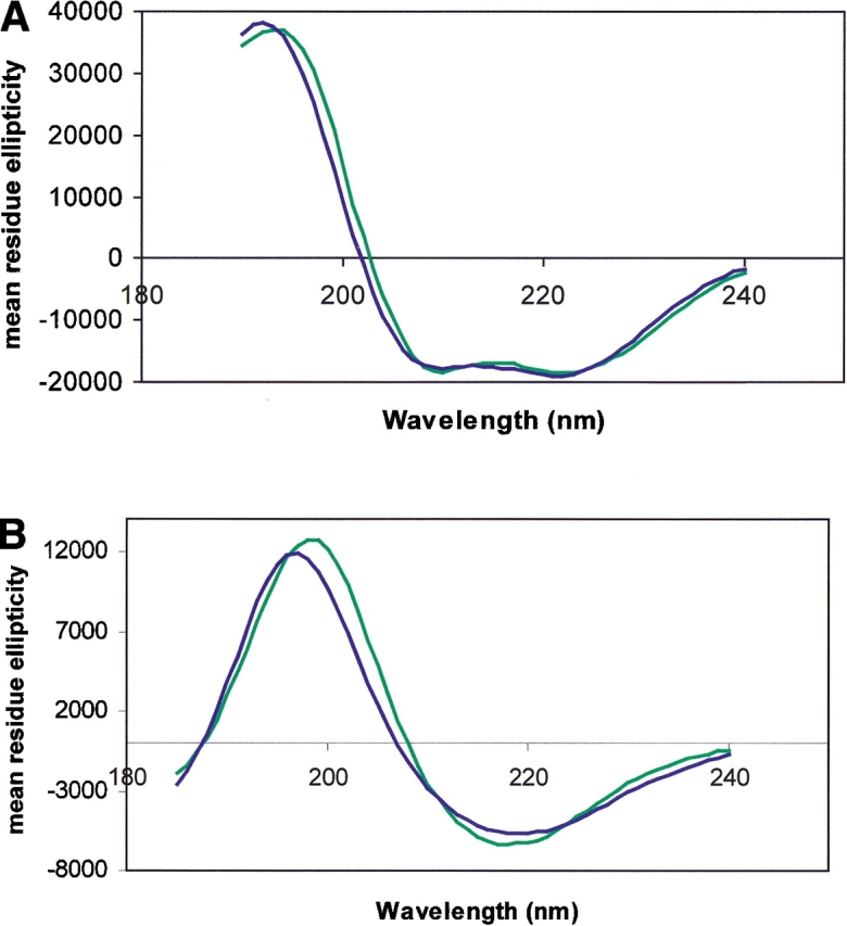
(A) Back-calculated spectrum (blue) for the lowest R_av solution (SELCON7) for MscL compared with the experimental spectrum (green). (B) Back-calculated spectrum (blue) for the lowest R_av solution (SELCON6) for FepA compared with the experimental spectrum (green).

Most importantly, there appears to be little or no correlation between the methods/databases that produced the best fits and the ones that produced the best results for the membrane proteins, unlike the case for soluble proteins. Therefore, in the absence of prior knowledge of the structure, there would have been no way to select among the methods and reference databases to obtain an accurate analysis.

Discussion

Membrane proteins are a class of proteins whose crystal structures have proved difficult to determine. As a result, only very few membrane protein structures have been solved to date (and many of these are closely related structures) compared to more than 10,000 soluble protein structures available in the PDB. CD spectroscopy has a potential role to play in the future in fold recognition studies and as a means of target selection for structural genomics programs (Wallace and Janes 2001), in addition to its traditional usage as a method for determining secondary structures and as a test for modelling studies of proteins with as yet unknown structures. For all of these types of studies, it is important that the secondary structures derived from the CD data accurately reflect the structures present in the proteins.

From the present study and a number of previous studies described in the literature (e.g., Johnson 1999^; Sreerama and Woody 2000), it can be seen that nearly all the methods and reference databases produce reasonable results for the soluble proteins tested, and that the various methods for calculating secondary structures from PDB files give reasonable agreement with the spectroscopic data.

However, for this admittedly limited (by necessity) survey of membrane proteins, the results are very different. First, the soluble and membrane proteins examined in this study have somewhat different spectral characteristics (peak shifts and to a lesser extent, the relative magnitudes of the individual exciton peaks). Second, the effects such features have on the accuracy of the secondary structures calculated using empirical methods with reference databases composed of soluble protein spectra have been explored. It is very clear that, although in some other cases the reference databases may be able to produce reasonably acceptable solutions, in ALL of the examples examined in this study, the reference databases derived from soluble proteins do not produce accurate results when applied to membrane protein CD spectral analyses. Furthermore, and most importantly, there does not appear to be a correlation between goodness of fit and correctness of structure, so there is no way to determine which method and database would be the most appropriate for the analysis of a particular membrane protein. Although the solvent shift phenomenon is likely to be one of the reasons for the discrepancies, the differences in membrane protein and soluble protein spectra cannot be explained simply, and so must be corrected for empirically.

One obvious conclusion from this study is that the availability of a reference database derived from membrane proteins could improve the analyses of membrane protein secondary structures by CD spectroscopy. We have begun to assemble such a database from as many membrane proteins as possible whose crystal structures have been solved, including a representative range of secondary structural types, with the intent of including these as an alternative reference database in DICHROWEB (Lobley et al. 2002).

Materials and methods

Materials

Horse myoglobin (Mb) (ICN Biochemicals Inc.) and concanavalin A (ConA) (Sigma) were dissolved in deionised water. Bacteriorhodopsin (BR) (a gift of P. Booth, Bristol University, UK) was dissolved in 1% octyl glucoside, the detergent used in the crystallization. The other proteins were provided by crystallographic labs and examined in the buffers used for crystallization: mechanosensitive channel (MscL) from M. tuberculosis (Chang et al. 1998); cytochrome oxidase (cox) from Paracoccus denitrificans complexed with a monoclonal antibody F_v fragment (Ostermeir et al. 1997); cytochrome bc₁ (cytbc₁) from bovine mitochrondria (Iwata et al. 1998); ferric enterobactin receptor (FepA; Buchanan et al. 1999); ferric hydroxamate uptake receptor (FhuA; Ferguson et al. 1998); maltoporin (LamB; Wang et al. 1997); and matrix porin (OmpF; Cowan et al. 1992).

For the mostly helical proteins, the concentrations used were ~5–7 mg/mL. The β-strand proteins were examined, in general, at higher concentrations (~18–30 mg/mL) due to the less intense nature of the β-strand CD signal.

CD spectroscopy

The conventional CD measurements were made on an Aviv 62ds instrument, which has a large angle detection geometry (for potentially scattering samples such as membrane proteins). The instrument was calibrated with d-camphour sulphonic acid for optical rotation and benzene vapor for wavelength. Data was collected at 0.2-nm intervals, and at 10°C, using a temperature-controlled chamber.

Suprasil cells (0.001-cm pathlength; Hellma UK Ltd.) were used for all the measurements (except for the FhuA sample, which was measured by SRCD at ~10 mg/mL in a 0.002-cm cell). Baselines were either water or the respective detergent/buffer solutions in which the proteins were dissolved.

At least four repeat scans were obtained for each sample and its respective baseline. The averaged baseline spectrum was subtracted from the averaged sample spectrum and the net spectrum smoothed with a Savitsky-Golay filter (Savitsky and Golay 1964).

Measurements were only made down to wavelengths where the instrument dynode voltage indicated the detector was still in its linear range. For myoglobin and ConA, this was 178 nm; for cytochrome oxidase it was 180 nm.

SRCD spectroscopy

Spectra were collected on Beamline 3.1 at Daresbury Laboratory, a part of the Centre for Protein and Membrane Structure and Dynamics (CPMSD), using a similar protocol and procedure to that described above for the conventional CD measurements. The SRCD was calibrated with d-camphour sulphonic acid for optical rotation and wavelength. Mb, ConA, and cox samples were measured using both CD and SRCD instruments, as controls. By comparison with the conventional CD data, the higher intensity of the light source permitted the SRCD data on Mb and ConA to be collected to 160 and 164 nm, respectively, and on cox to 169 nm.

Calculations of MRE and delta epsilon values

To calculate the mean residue ellipticities (MRE), the protein concentrations were determined by duplicate quantitative amino acid analysis, and the mean residue weights used were as follows: 110 (Mb); 108 (ConA); 111 (cox); 108 (BR); 111 (cytbc₁); 111 (MscL); 110 (FepA); 110 (FhuA); 113 (LamB); 109 (OmpF). Δɛ was calculated as MRE/3298.

Secondary structure calculations from crystal structures

The following programs were used to calculate secondary structural contents from the relevant PDB files: PROCHECK (Laskowski et al. 1993), DSSP (Kabsch and Sander 1983), XtlSSTR (King and Johnson 1999), PROMOTIF (Hutchinson and Thornton 1996), and Stride (Frishman and Argos 1995). The various programs define different types of secondary structures, so to enable more facile comparisons to be made, the various types of helical structures have been grouped together, as have the diverse types of sheets and turns, resulting in only four broad categories of structures: helix, sheet, turn, and other. If the PDB file had missing or disordered (undefined) residues, the percentages calculated were for the residues forming the defined secondary structures divided by the total number of residues in the protein. If there was more than one appropriate crystal structure for the protein available, the highest resolution PDB file was used.

The PDB files used were: 1DWT (Mb), 1NLS (ConA), 1MSL (MscL), 1AR1(cox), 1BGY (cytbc₁), 1C3W (BR), 1FEP (FepA), 2FCP (FhuA), 1AF6 (LamB), and 2OMF (OmpF).

Secondary structure analyses of CD data

Most of the secondary structural analyses used DICHROWEB (http://www.cryst.bbk.ac.uk/cdweb) an interactive Web server (Lobley and Wallace 2001; Lobley et al. 2002) that permits analyses via the following methods: SELCON3 (Sreerama and Woody 1993; Sreerama et al. 1999), CONTIN (Provencher and Glockner 1981; van Stokkum et al. 1990), and CDSSTR (Sreerama and Woody 2000), with a wide range of protein spectral databases (all derived from soluble proteins; Sreerama and Woody 2000^; Sreerama et al. 2000). CDPro (Sreerama and Woody 2000) was used for analyses comparing the effect of including or excluding Mb and ConA in the reference databases. VARSLC (Compton and Johnson 1986; Manalavan and Johnson 1987) and K2D (Andrade et al. 1993) were used with their standard reference databases. The VARSLC results reported used the default parameters, but very similar results (data not shown) were obtained using other parameters with this method.

As a means of comparison of the goodness of fit of the various methods, the normalized root-mean-square deviation (NRMSD) parameter (Mao et al. 1982) was calculated for all of the analyses except VARSLC, which does not produce reconstituted spectra. NRMSD is defined as: Σ[(θexp − θcal)²/(θexp)²]^½, summed over all wavelengths, where θexp and θcal are, respectively, the experimental ellipticities and the ellipticities of the back-calculated spectra for the derived structure. NRMSD values of <0.1 mean that the back-calculated and experimental spectra are in close agreement (Brahms and Brahms 1980). A low NRSMD is not sufficient to indicate a correct analysis, but a poor (high) NRMSD generally indicates the analysis is problematic.

For each of the analyses, several types of R parameters were calculated as measures of the correspondence between the crystal structure and the structure calculated from the CD data. These were defined as: R = ∑[f_Xray − f_CD], summed over helical, sheet and turn secondary structure types, where f_Xray and f_CD are the fractions of a given secondary structural type derived from the Xray structure or calculated by the CD method, respectively. Values of R were calculated using both the average Xray (R_av) structure derived from all methods, and the X-ray structure calculated by XtlSSTR (R_xs). R_P was calculated for the principal type of secondary structure present (i.e., helix for primarily helical structures, sheet for primarily sheet structures) using the averaged values for the secondary structures. Low R-values mean that the analyses have been successful.

Abbreviations

• CD, circular dichroism

• SRCD, synchrotron radiation circular dichroism

• Mb, myoglobin

• ConA, concanavalanA

• BR, bacteriorhodopsin

• MscL, mechanosensitive channel

• cox, cytochrome oxidase

• cytbc1, cytochrome bc₁

• FepA, ferric enterobactin receptor

• FhuA, ferric hydroxamate uptake receptor

• LamB, maltoporin

• OmpF, matrix porin

• NRMSD, normalized root-mean-square deviation (goodness-of-fit parameter)

• PDB, Protein Data Bank

References

- Andrade, M.A., Chacón, P., Merelo, J.J., and Morán, F. 1993. Evaluation of secondary structure of proteins from UV circular dichroism using an unsupervised learning neural network. Protein Eng. 6 383–390. [DOI] [PubMed] [Google Scholar]
- Blundell, T.L. and Mizuguchi, K. 2000. Structural genomics: An overview. Prog. Biophys. Mol. Biol. 73 289–295. [DOI] [PubMed] [Google Scholar]
- Brahms, S. and Brahms, J. 1980. Determination of protein secondary structure in solution by vacuum ultraviolet circular dichroism. J. Mol. Biol. 138 149–178. [DOI] [PubMed] [Google Scholar]
- Buchanan, S.K., Smith, B.S., Venkatramani, L., Xia, D., Esser, L., Palnitkar, M., Chakraborty, R., van der Helm, D., and Deisenhofer, J. 1999. Crystal structure of the outer membrane active transporter FepA from Escherichia coli. Nat. Struct. Biol. 6 56–63. [DOI] [PubMed] [Google Scholar]
- Cascio, M. and Wallace, B.A. 1994. Red- and blue-shifting in the circular dichroism spectra of polypeptides due to dipole effects. Protein Pept. Lett. 1 136–140. [Google Scholar]
- ———. 1995. Effects of local environment on the circular dichroism spectra of polypeptides. Anal. Biochem. 227 90–100. [DOI] [PubMed] [Google Scholar]
- Chang, C.T., Wu, C.S., and Yang, J.T. 1978. Circular dichroism analysis of protein conformation: Inclusion of the β-turns. Anal. Biochem. 91 13–31. [DOI] [PubMed] [Google Scholar]
- Chang, G., Spencer, R.H., Lee, A.T., Barclay, M.T., and Rees, D.C. 1998. Structure of the MscL homologue from Mycobacterium tuberculosis: A gated mechanosensitive ion channel. Science 282 2220–2226. [DOI] [PubMed] [Google Scholar]
- Chen, Y. and Wallace, B.A. 1997a. Secondary solvent effects on the circular dichroism spectra of polypeptides: Influence of polarisation effects on the far ultraviolet spectra of alamethicin. Biophys. Chem. 65 65–74. [DOI] [PubMed] [Google Scholar]
- ———. 1997b. Solvent effects on the conformation and far ultraviolet circular dichroism spectra of gramicidin A. Biopolymers 42 771–781. [DOI] [PubMed] [Google Scholar]
- Compton, L.A. and Johnson, Jr., W.C. 1986. Analysis of protein circular dichroism spectra for secondary structure using a simple matrix multiplication. Anal. Biochem. 155 155–167. [DOI] [PubMed] [Google Scholar]
- Cowan, S.W., Schirmer, T., Rummel, G., Steiert, M., Ghosh, R., Pauptit, R.A., Jansonius, J.N., and Rosenbusch, J.P. 1992. Crystal structures explain functional properties of 2 Escherichia coli porins. Nature 358 727–733. [DOI] [PubMed] [Google Scholar]
- Ferguson, A.D., Hofmann, E., Coulton, J.W., Diederichs, K., and Welte, W. 1998. Siderophore-mediated iron transport: Crystal structure of FhuA with bound lipopolysaccharide. Science 282 2215–2220. [DOI] [PubMed] [Google Scholar]
- Frishman, D. and Argos, P. 1995. Knowledge-based protein secondary structure assignment. Proteins Struct. Funct. Genet. 23 566–579. [DOI] [PubMed] [Google Scholar]
- Hutchinson, E.G. and Thornton, J.M. 1996. PROMOTIF—A program to identify structural motifs in proteins. Protein Sci. 5 212–220. [DOI] [PMC free article] [PubMed] [Google Scholar]
- Iwata, S., Lee, J.W., Okada, K., Lee, J.K., Iwata, M., Rasmussen, B., Link, T.A., Ramaswamy, S., and Jap, B.K. 1998. Complete structure of the 11-subunit bovine mitochondrial cytochrome bc1 complex. Science 281 64–71. [DOI] [PubMed] [Google Scholar]
- Johnson, Jr., W.C. 1999. Analyzing protein CD for accurate secondary structures. Proteins Struct. Funct. Genet. 35 307–312. [PubMed] [Google Scholar]
- Kabsch, W. and Sander, C. 1983. Dictionary of protein secondary structure: Pattern recognition of hydrogen-bonded and geometrical features. Biopolymers 22 2577–2637. [DOI] [PubMed] [Google Scholar]
- King, S.M. and Johnson, Jr., W.C. 1999. Assigning secondary structure from protein coordinate data. Proteins Struct. Funct. Genet. 35 313–320. [PubMed] [Google Scholar]
- Laskowski, R.A., MacArthur, M.W., Moss, D.S., and Thornton, J.M. 1993. PROCHECK—A program to check the stereochemical quality of protein structures. J. Appl. Crystallogr. 26 283–291. [Google Scholar]
- Lees, J.G. and Wallace, B.A. 2002. Synchrotron radiation circular dichroism and conventional circular dichroism spectroscopy: A comparison. Spectroscopy 16 121–125. [Google Scholar]
- Lobley, A. and Wallace, B.A. 2001. DICHROWEB: A website for the analysis of protein secondary structure from circular dichroism spectra. Biophys. J. 80 373a. [DOI] [PubMed] [Google Scholar]
- Lobley, A., Whitmore, L., and Wallace, B.A. 2002. DICHROWEB: An interactive website for the analysis of protein secondary structure from circular dichroism spectra. Bioinformatics 18 211–212. [DOI] [PubMed] [Google Scholar]
- Mao, D. and Wallace, B.A. 1984. Differential light scattering and absorption flattening optical effects are minimal in the circular dichroism spectra of small unilamellar vesicles. Biochemistry 23 2667–2673. [DOI] [PubMed] [Google Scholar]
- Mao, D., Wachter, E., and Wallace, B.A. 1982. Folding of the H+-ATPase proteolipid in phospholipid vesicles. Biochemistry 21 4960–4968. [DOI] [PubMed] [Google Scholar]
- Ostermeier, C., Harrenga, A., Ermler, U., and Michel, H. 1997. Structure at 2.7 A resolution of the Paracoccus denitrificans two-subunit cytochrome c oxidase complexed with an antibody FV fragment. Proc. Natl. Acad. Sci. 94 10547–10553. [DOI] [PMC free article] [PubMed] [Google Scholar]
- Pancoska, P. and Keiderling, T.A. 1991. Systematic comparison of statistical analysis of electronic and vibrational circular dichroism for secondary structure prediction of selected proteins. Biochemistry 30 6885–6895. [DOI] [PubMed] [Google Scholar]
- Pancoska, P., Blazek, M., and Keiderling, T.A. 1992. Relationships between secondary structure fractions for globular proteins. Neural network analyses of crystallographic data sets. Biochemistry 31 10250–10257. [DOI] [PubMed] [Google Scholar]
- Provencher, S.W. and Glockner, J. 1981. Estimation of globular protein secondary structure from circular dichroism. Biochemistry 20 33–37. [DOI] [PubMed] [Google Scholar]
- Savitsky, A. and Golay, M.J.E. 1964. Smoothing and differentiation of data by simplified least squares procedures. Anal. Chem. 36 1627–1639 [DOI] [PubMed] [Google Scholar]
- Sreerama, N. and Woody, R.W. 1993. A self-consistent method for the analysis of protein secondary structure from circular dichroism. Anal. Biochem. 209 32–44. [DOI] [PubMed] [Google Scholar]
- ———. 2000. Estimation of protein secondary structure from CD spectra: Comparison of CONTIN, SELCON and CDSSTR methods with an expanded reference set. Anal. Biochem. 282 252–260. [DOI] [PubMed] [Google Scholar]
- Sreerama, N., Venyaminov, S.Y., and Woody, R.W. 1999. Estimation of the number of helical and strand segments in proteins using CD spectroscopy. Protein Sci. 8 370–380. [DOI] [PMC free article] [PubMed] [Google Scholar]
- ———. 2000. Estimation of protein secondary structure from CD spectra: Inclusion of denatured proteins with native protein in the analysis. Anal. Biochem. 287 243–251. [DOI] [PubMed] [Google Scholar]
- Teeters, C.L., Eccles, J., and Wallace, B.A. 1987. A theoretical analysis of the effects of sonication on differential absorption flattening in suspensions of membrane sheets. Biophys. J. 51 527–532. [DOI] [PMC free article] [PubMed] [Google Scholar]
- Toumadje, A., Alcorn, S.W., and Johnson, Jr., W.C. 1992. Extending CD spectra of proteins to 168 nm improves the analysis for secondary structure. Anal. Biochem. 200 321–331. [DOI] [PubMed] [Google Scholar]
- van Stokkum, I.H.M., Spoelder, H.J.W., Bloemendal, M., van Grondelle, R., and Groen, F.C.A. 1990. Estimation of protein secondary structure and error analysis from CD spectra. Anal. Biochem. 191 110–118. [DOI] [PubMed] [Google Scholar]
- Wallace, B.A. 2000. Synchrotron radiation circular-dichroism spectroscopy as a tool for investigating protein structures. J. Synchrotron Radiation 7 289–295. [DOI] [PubMed] [Google Scholar]
- Wallace, B.A. and Janes, R.W. 2001. Synchrotron radiation circular dichroism spectroscopy of proteins: Secondary structure, fold recognition, and structural genomics. Curr. Opin. Chem. Biol. 5 567–571. [DOI] [PubMed] [Google Scholar]
- Wallace, B.A. and Mao, D. 1984. Circular dichroism analyses of membrane proteins: An examination of light scattering and absorption flattening in large membrane vesicles and membrane sheets. Anal. Biochem. 142 317–328. [DOI] [PubMed] [Google Scholar]
- Wallace, B.A. and Teeters, C.L. 1987. Differential absorption flattening optical effects are significant in the circular dichroism spectra of large membrane fragments. Biochemistry 26 65–70. [DOI] [PubMed] [Google Scholar]
- Wallace, B.A., Kohl, N., and Teeter, M. 1984. Crambin in phospholipid vesicles: Circular dichroism analysis of crystal structure relevance. Proc. Natl. Acad. Sci. 81 1406–1410. [DOI] [PMC free article] [PubMed] [Google Scholar]
- Wang, Y.F., Dutzler, R., Rizkallah, P.J., Rosenbusch, J.P., and Schirmer, T. 1997. Channel specificity: Structural basis for sugar discrimination and differential flux rates in maltoporin. J. Mol. Biol. 272 56–63. [DOI] [PubMed] [Google Scholar]
- Woody, R.W. 1995. Circular dichroism. Methods Enzymol. 246 34–71. [DOI] [PubMed] [Google Scholar]