A graph-theory algorithm for rapid protein side-chain prediction

Abstract

Fast and accurate side-chain conformation prediction is important for homology modeling, ab initio protein structure prediction, and protein design applications. Many methods have been presented, although only a few computer programs are publicly available. The SCWRL program is one such method and is widely used because of its speed, accuracy, and ease of use. A new algorithm for SCWRL is presented that uses results from graph theory to solve the combinatorial problem encountered in the side-chain prediction problem. In this method, side chains are represented as vertices in an undirected graph. Any two residues that have rotamers with nonzero interaction energies are considered to have an edge in the graph. The resulting graph can be partitioned into connected subgraphs with no edges between them. These subgraphs can in turn be broken into biconnected components, which are graphs that cannot be disconnected by removal of a single vertex. The combinatorial problem is reduced to finding the minimum energy of these small biconnected components and combining the results to identify the global minimum energy conformation. This algorithm is able to complete predictions on a set of 180 proteins with 34,342 side chains in <7 min of computer time. The total χ₁ and χ_{1 + 2} dihedral angle accuracies are 82.6% and 73.7% using a simple energy function based on the backbone-dependent rotamer library and a linear repulsive steric energy. The new algorithm will allow for use of SCWRL in more demanding applications such as sequence design and ab initio structure prediction, as well addition of a more complex energy function and conformational flexibility, leading to increased accuracy.

Protein structure prediction by homology modeling or ab initio methods remains a difficult challenge. An important component of any modeling method is the prediction of side-chain conformations. Side-chain prediction usually entails placing side chains onto fixed backbone coordinates either obtained from a parent structure or generated from ab initio modeling simulations or a combination of these. Many side-chain prediction methods have been presented in the past 15 years (Summers and Karplus 1989; Holm and Sander 1991; Lee and Subbiah 1991; Tuffery et al. 1991; Desmet et al. 1992, 2002; Dunbrack and Karplus 1993; Wilson et al. 1993; Kono and Doi 1994; Laughton 1994; Hwang and Liao 1995; Koehl and Delarue 1995; Bower et al. 1997; Samudrala and Moult 1998; Dunbrack 1999; Mendes et al. 1999a; Xiang and Honig 2001; Liang and Grishin 2002).

Nearly all of these are based on using a rotamer library of discrete side-chain conformations (McGregor et al. 1987; Ponder and Richards 1987; Tuffery et al. 1991; Dunbrack and Karplus 1993, 1994; De Maeyer et al. 1997; Dunbrack and Cohen 1997; Lovell et al. 2000; Xiang and Honig 2001; Dunbrack 2002) obtained from statistical analysis of the Protein Data Bank (PDB; Berman et al. 2000). Rotamer libraries can either be backbone-independent or backbone-dependent. Backbone-dependent rotamer libraries contain information on side-chain dihedral angles and rotamer populations as a function of the backbone dihedral angles φ and ψ (Dunbrack and Karplus 1993, 1994; Dunbrack and Cohen 1997; Dunbrack 2002), whereas backbone-independent libraries ignore such dependence.

In side-chain prediction methods, rotamers are chosen based on the desired protein sequence and the given backbone coordinates, by using a defined energy function and search strategy. Energy functions that have been used in side-chain prediction include simple steric energy functions combined with log probabilities of backbone-dependent rotamer populations (Dunbrack 1999), as well as molecular mechanics potential energy functions with complex solvation free energy terms (Mendes et al. 2001a; Xiang and Honig 2001; Liang and Grishin 2002).

For some emerging uses of side-chain prediction, fast calculations are a requirement. These include Web-based homolog and fold-recognition programs that align query sequences to proteins of known structure and model proteins based on these identifications and alignments. For instance, 3D-PSSM (Kelley et al. 2000) uses SCWRL (Bower et al. 1997) to generate models of proteins from structure-derived profile alignments. As the numbers of available sequences and experimentally determined protein structures both increase, improved models of proteins can be constructed on the basis of a number of parent structures and many alternative alignments, as demonstrated at the recent CASP5 meeting. In some cases, hundreds of models can be used to determine the best parent and alignment for a single query sequence, thus necessitating fast side-chain prediction. The protein design problem, in which a sequence is designed that will fold into a given defined set of backbone coordinates (Desjarlais and Handel 1995; Dahiyat and Mayo 1996) also requires efficient side-chain search methods, because several residue types and many rotamers must be tested at every site of the protein. In this case, the combinatorial problem can be quite severe.

A search method used in side-chain prediction can be classified as either exact or approximate, depending on whether it is guaranteed to find the global minimum energy given the rotamer library and energy function, or instead whether it finds a low-energy conformation without such a guarantee. The many versions of the dead-end elimination algorithm (Desmet et al. 1992, 1997; Lasters and Desmet 1993; Goldstein 1994; Keller et al. 1995; Lasters et al. 1995; Gordon and Mayo 1999; Pierce et al. 1999; De Maeyer et al. 2000; Voigt et al. 2000; Looger and Hellinga 2001) are designed to find the global minimum energy, when they are able to converge. Conversely, Monte Carlo methods (Holm and Sander 1991; Liang and Grishin 2002), cyclical search methods (Dunbrack and Karplus 1993; Xiang and Honig 2001), and some other algorithms (Desmet et al. 2002) are not guaranteed to find a global minimum, but they will almost always find a low-energy conformation in a reasonable time.

We have continued to develop the SCWRL program, originally written by Michael Bower, over a number of years (Bower et al. 1997; Dunbrack 1999). SCWRL uses a backbone-dependent rotamer library (Dunbrack and Karplus 1993, 1994; Dunbrack and Cohen 1997; Dunbrack 2002) and an energy function based on log probabilities of these rotamers and a simple repulsive steric energy term. In this article, we will present a new algorithm for SCWRL based on graph theory, which is considerably faster than the original algorithm. The new algorithm will enable new uses such as protein design and ab initio structure prediction, as well as increases in accuracy with new energy functions and side-chain flexibility.

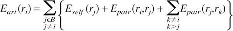
Before describing the new algorithm, it is useful to summarize the previous method used to solve the side-chain combinatorial problem in SCWRL as well as its drawbacks. The original SCWRL algorithm initially places side chains onto the backbone according to the backbone-dependent rotamer probabilities and steric interactions with the nonlocal backbone. Any side chains that clash with other side chains according to the steric energy function are then defined as "active." These active residues are placed in each of their possible rotamers in turn, and if any rotamer clashes with any currently "inactive" residues, these residues become active as well. This procedure continues until a set of active residues is identified. The combinatorial problem is reduced to finding the minimum energy configuration of these active residues, because the inactive residues are in their minimum energy conformation. This is de facto a dead-end elimination of all rotamers except one for each inactive residue.

We can represent the side-chain combinatorial problem in terms of graph theory by making each residue a vertex in an undirected graph. If at least one rotamer of residue i interacts with at least one rotamer of residue j, then there is an edge between vertices i and j of the graph. In the original SCWRL algorithm, the active residues can be represented as a graph, one that is not necessarily connected. The active residues can therefore be grouped into interacting clusters. Residues in different clusters do not have contacts with one another. Each cluster is a connected subgraph of the entire graph. The combinatorial problem is therefore reduced to enumerating the combinations of rotamers for the residues in each connected graph. In SCWRL, the lowest energy of each cluster is found by using a backtracking algorithm with pruning (see Materials and Methods).

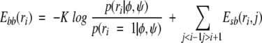
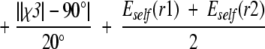
Some clusters are too large to be solved in a reasonable period of time. The solution to this problem (Bower et al. 1997) is to locate one residue (the "keystone") that when removed from the cluster graph, breaks the graph into two separate subgraphs. This procedure is shown in Figure 1A ▶. Assuming each residue has the same number of rotamers, n_rot, the number of combinations in this graph, is n¹¹_rot. The graph in Figure 1A ▶ has one residue labeled as a dark gray vertex that breaks the graph into two pieces when removed, as shown on the lower part of the figure. The global minimum of the energy can be found by identifying the minimum energy configuration for each subgraph once for each rotamer of the keystone residue. The solution is the one that finds the minimum energy using the equation

(1)

where E_L(r_i) = ^min_{{rj,jɛL,j≠i}} E({r_j}│r_i) is the lowest energy combination of rotamers in the left subgraph (L) with the keystone residue i fixed in rotamer r_i, and E_R is the term for the right subgraph. E_self (r_i) is the energy of interaction of the side chain with the backbone and other fixed non–side-chain atoms, such as ligands. Splitting the graph results in n⁵_rot + n⁷_rot combinations. This process may result in subgraphs that are also too large to be solved in a reasonable time. SCWRL breaks these up by using a similar procedure, so that each subgraph is broken up for each rotamer of the first keystone residue and then for each rotamer of the second keystone residue, and so on.

Figure 1.

Splitting clusters into components. (A) Splitting a cluster into two components in SCWRL2.95 and earlier versions of SCWRL. (B) Splitting a cluster into biconnected components in SCWRL3.0. First-order articulation points are in light gray, and the second-order articulation point is in dark gray.

In addition to the challenges described above for side-chain prediction, there are a number of other reasons for developing a new algorithm for SCWRL. First, when the backbone used for modeling is not the native backbone structure for the protein, the connectedness of side chains (i.e., the average number of edges per node in the graph) may be higher than for native backbones, because in general, there may not be sufficient volume available for all side chains. This is especially true at low sequence identity and in ab initio modeling, when backbone structures very different from the native are generated. For a small proportion of target structures to be modeled, SCWRL may not converge in any reasonable amount of time. Second, to improve SCWRL accuracy, it is likely to be necessary to implement an energy function that includes favorable van der Waals interactions, as well as electrostatic and solvation energy terms (Liang and Grishin 2002). Flexibility of side chains may also be necessary to improve the accuracy of large hydrophobic residues (Mendes et al. 1999a). These changes will make the connectedness problem even worse, and the current SCWRL algorithm is not robust enough to find a solution.

Third, SCWRL also uses a number of heuristic steps to reduce the number of rotamers and the number of interactions considered in the cluster-solving algorithm. These include removing rotamers with backbone (local and nonlocal) energies >5.0 kcal/mole, and not forming edges between residues in the graph unless there is some pair of rotamers with interaction energy >10.0 kcal/mole. The effect of using these heuristics is that SCWRL does not locate the global energy minimum of its own energy function, because many interactions are ignored when setting up the combinatorial searches to make the calculations tractable.

In this article, we propose a new algorithm for SCWRL based on graph theory that overcomes the combinatorial problem in a novel way, as illustrated in Figure 1B ▶. Instead of recursively breaking up graphs into pieces as in previous versions of SCWRL (Fig. 1A ▶), the new algorithm breaks up clusters of interacting side chains into the biconnected components of an undirected graph. Biconnected graphs are those that cannot be broken apart by removal of a single vertex. Biconnected graphs are cycles, nested cycles, or a single pair of residues connected by an edge (sometimes referred to as a bridge). In Figure 1B ▶, the graph in Figure 1A ▶ is shown, before and after being broken up into biconnected components. This graph can be broken up into five biconnected components: A is residues V10, R15, Y21, and K17; B is residues K17 and T30; C is residues T30, Q25, M32, H29, and W11; D is residues W11 and F35; and E is residues W11 and D39.

Vertices that appear in more than one biconnected component are called "articulation points." Removing an articulation point from a graph breaks the graph into two separate subgraphs. In this graph, vertices K17, T30, and W11 are articulation points. The order of an articulation point is the number of biconnected components of which it is a member minus one. A first-order articulation point connects only two components. Both K17 and T30 are first-order articulation points (Fig. 1B ▶, light gray), whereas residue W11 is a second-order articulation point (Fig. 1B ▶, dark gray). Finding biconnected components and their articulation points is easily accomplished by using an algorithm developed by Tarjan (1972). The algorithm uses a standard depth-first search algorithm from graph theory contained in many computer science textbooks.

To solve the side-chain combinatorial problem with biconnected components, we use the following simple procedure, illustrated in Figure 2 ▶. For each biconnected component with only one articulation point, we find the minimum energy over all combinations of rotamers of the residues in the component for each rotamer of the articulation point. This energy includes all interactions among these residues and between these residues and the fixed rotamer of the articulation point. So in the first panel of Figure 2 ▶, we calculate the minimum energy over all combinations of rotamers of residues V10, R15, and Y21 for each rotamer of residue K17. Once this is accomplished, we can collapse the biconnected component onto the articulation point, obtaining the graph in the second panel of Figure 2 ▶. That is, we can now consider residue K17 a superresidue with a number of superrotamers. If residue K17 has 10 rotamers, superresidue {K17, V10, R15, Y21} also has 10 rotamers. The energies of these superrotamers include both the self-energies of residue K17 and the minimum energy of the biconnected component consisting of residues V10, R15, and Y21. After collapse, we reduce the order of articulation point K17 by one, so it is now no longer an articulation point in the second panel (i.e., is of zeroth order).

Figure 2.

Solving a cluster by using biconnected components. The minimum energy configuration of the cluster shown in Figure 1 ▶ is identified by stepwise solution of biconnected components. Each biconnected component is solved as shown in the right margin, and the collapsed component is shown as superresidues in curly brackets.

We now proceed to another component with only one articulation point, for instance, component E. We find the minimum energy of E for each rotamer of W11 and collapse the component onto W11, making it the superresidue {W11, D39}, resulting in the third panel of Figure 2 ▶. After collapse, W11 is now of first order. We can also solve component D for each rotamer of articulation point W11, resulting in the superresidue {W11, D39, F35}. W11 is now no longer an articulation point (Fig. 2 ▶, fourth panel).

At this point, after collapsing several biconnected components, we have two components that now have only one articulation point, whereas before they had two each. We solve the first one, B, for each rotamer of residue T30 and form the superresidue {T30, K17, V10, R15, Y21}. We are left with one biconnected component with no articulation points. We find the minimum energy of this component over all combinations of its rotamers.

The procedure as just described always converges into a single biconnected component or a single residue, each rotamer of which now contains information about all other residues in the cluster as well as the total energy. The order of complexity of the side-chain problem is now reduced to the size of the largest biconnected component in any cluster.

To achieve reasonably sized biconnected components, the new program, referred to here as SCWRL3.0, begins with a dead-end elimination (DEE) step, based on the simple Goldstein criterion (Goldstein 1994). This DEE step replaces the heuristics in SCWRL previously used to remove many high-energy rotamers not likely to be part of the minimum-energy configuration. Because the simple DEE criterion is not sufficient to solve the combinatorial problem on its own for reasonably sized proteins, a number of recent papers have presented complex DEE schedules that remove clusters of rotamers. However, the new SCWRL algorithm based on biconnected components stands in contrast to recent DEE implementations (Pierce et al. 1999; De Maeyer et al. 2000; Looger and Hellinga 2001) in its simplicity and speed.

We show that the new algorithm is extremely fast even for very large proteins. We evaluate the accuracy and speed of the new algorithm, as implemented in SCWRL3.0. The new algorithm will allow for new applications and for the development of more accurate energy functions and consideration of side-chain flexibility without a significant impact on computational times.

Materials and methods

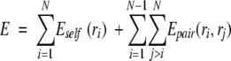
Outline of the procedure

The full procedure for side-chain prediction in SCWRL3.0 consists of a number of steps that are described more fully below.

Step 1: Input

Read in backbone coordinates and (optionally) a new sequence file and ligand coordinates. Measure backbone φ and ψ dihedral angles from the input coordinates, checking for chain connectivity.

Step 2: Rotamers

For each residue, read in rotamer dihedral angles and probabilities from binary-formatted backbone-dependent rotamer library, given measured values of φ and ψ and the amino acid type. Currently rotamers are read in from highest to lowest probability until the cumulative density reaches at least 90% for each residue. Calculate cartesian coordinates for rotamers of all side chains, and calculate side-chain/backbone energy terms

(2)

where the first term is derived from the backbone-dependent rotamer probability given φ and ψ, and the second term consists of the interactions of the side-chain rotamer r_i of residue i with the backbone of all residues further than one amino acid away in the sequence. The backbone-dependent rotamer library is assumed to take care of the backbone/side-chain interactions of residue i with itself and its neighbors one residue away. Determine which pairs of side chains may be able to interact given the distance between their Cβ atoms and the maximum distance of any atom in the side chain from its Cβ. These distances have been calculated from data in the PDB used in the backbone-dependent rotamer library.

Step 3: Disulfides

If desired, determine likely disulfide pairings (see below). Fix Cys side chains that are designated disulfides for the rest of the calculation.

Step 4: Dead-end elimination

Perform a DEE of rotamers that cannot be part of the global minimum energy configuration by using the "Goldstein criterion." The Goldstein criterion is the simplest version of DEE. If the total energy for all side chains is expressed as the sum of self and pairwise energies,

(3)

then a rotamer s_i can be eliminated from the search if there is another rotamer r_i for the same side chain that satisfies the following equation:

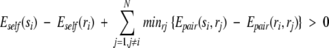(4)

In words, rotamer s_i of residue i can be eliminated from the search if another rotamer of residue i, r_i, always has a lower interaction energy with all other side chains and the backbone regardless of which rotamer is chosen for the other side chains. The DEE step can be made fairly efficient by applying the algorithm for rotamers from highest to lowest E_self, and once removed, a rotamer is not included in the minimum or sum steps in Equation 4. Residues that have only one rotamer left after the DEE step are fixed for the rest of the calculation. The energy of interaction of these fixed side chains (also including disulfide-bonded cysteines) with any unfixed side chains is added to the self-energy of the unfixed side chains. That is,

(5)

where

Step 5: Residue graph

Define residues that have more than one rotamer left after the DEE step as "active" residues. These residues can be viewed as the vertices of a graph that may or may or not be connected. The first step in solving the combinatorial problem of the active residues is to compute the edges among the active residue pairs. For every pair of residues, i,j, there is an edge if at least one energy, E_pair(r_i,r_j) ≠ 0. This does not necessarily mean checking every pair of rotamers, because as soon as one pair of interacting rotamers is found, then an edge is established, and the energies for other rotamer pairs for residue pair i,j do not need to be evaluated at this stage. Determine the interacting clusters of residues. That is, determine which sets of residues form connected graphs, given the list of edges.

Step 6: Biconnected components

For each cluster, determine the set of biconnected components and articulation points in the graph by sing a depth-first search procedure (see below; Tarjan 1972). The order of each articulation point is defined as N_bicon − 1, the number of biconnected components attached to the articulation point minus one. An articulation point that connects only two biconnected components is first order.

Step 7: Solve clusters

Find the minimum energy for each connected graph (cluster) in turn: For each biconnected component of the cluster with only one articulation point, find the energy minimum of the residues in the component for each rotamer of the articulation point. That is, the rotamer of the articulation point is fixed, and the rotamers of the other residues in the component are searched until the minimum energy is found. A branch-and-bound backtracking algorithm is used for this purpose (see below), in which the residues in the component are sorted from lowest to highest number of rotamers and the rotamers of each residue are sorted from lowest to highest self-energy. Store the lowest energy of the biconnected component as well as the rotamer identities with each rotamer of the articulation point. The articulation point rotamers now have a new energy component in their self energies—the energy of the biconnected component, B, which includes the self energies of these rotamers as well as their interactions with each other and with the articulation point rotamer, r_i,

(6)

The total self-energy for the articulation point rotamers is now

(7)

After a biconnected component is solved for each rotamer, the component can be collapsed so that the articulation point rotamers are now superrotamers, defined as a group of residues with one rotamer defined for each residue. The superrotamers have self-energies defined in Equation 7. After the collapse, we reduce the order of the articulation point by one. If the order is zero, then the residue is no longer an articulation point. After collapsing all biconnected components with only one articulation point and reducing the orders of these articulation points, additional biconnected components will have only one articulation point, as illustrated in Figure 2 ▶. These biconnected components are then solved in a similar fashion. The process of solving each biconnected component for the rotamers of its articulation point is performed until there is only one biconnected component left with no articulation points. This final component is solved with the branch-and-bound algorithm described below.

Step 8: Output

Print coordinates of the chosen rotamers, including the disulfides, the fixed side chains, and those solved in each of the clusters.

Articulation points and biconnected components

In Step 6 above, a cluster of interacting residues, represented as vertices in a graph, are broken up into biconnected components. In this process, the articulation points that connect the biconnected components are also identified. A vertex of a connected graph is an articulation point if its removal from the graph, together with all the edges incident from that vertex, would split the graph into two or more components, with no edges between them. If a graph does not contain any articulation point, it is defined as biconnected.

The procedure for identifying biconnected components and articulation points is described in a number of computer science textbooks. The first step involves a depth-first search, or tree traversal, in which each vertex of the graph is assigned a depth-first number (DFN), numbering the vertices in the order in which they are visited. This is illustrated in Figure 3 ▶. In a depth-first search, the vertices and edges of the graph are used to build a tree, in which each vertex may have several children, or descendants, connected by edges of the graph, and each vertex has a single parent, or ancestor. The nodes of the tree are searched by descending the tree as far as possible, before exploring additional nodes attached to each traversed vertex, in reverse order. For example, given the residue interaction graph from Figure 1B ▶, a depth-first traversal starting from residue V10 assigns the DFNs shown inside of the circles representing each node in Figure 3 ▶. In the figure, the edges that were used during depth-first tree traversal are drawn in continuous lines and are called tree edges, whereas the ones that were not traversed are called back edges and are drawn with dashed lines.

Figure 3.

Algorithm for splitting a graph into biconnected components. In the bottom part of the figure, the depth-first search numbers (DFN) are shown in the circles for each node, and the low numbers (L) are shown in shaded squares adjacent to each node. Inequalities between the DFNs and L numbers of adjacent residues that indicate the presence of articulation points (and also the root node) are shown.

In addition to the depth-first numbers, each vertex is assigned a low number, notated as L(u) and defined by

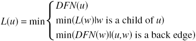(8)

In words, L(u) is the lowest DFN that can be reached from u using a path that includes only descendants of u and at most one back edge. In our example (Fig. 3 ▶), low numbers are printed within the square boxes near each node. A node u that has a child w that satisfies DFN(u) < L(w) is either the root node or an articulation point.

We implemented a recursive function ART that scans the tree and computes the L and DFNs. Also it stores all the traversed edges in a stack. If for a certain vertex the articulation point inequality is met, a new biconnected component is created. All the edges are popped off of the edge stack and the vertices of these edges are used to define a biconnected component. For each identified articulation point, we keep track of the number of biconnected components that it is part of. The algorithm is shown in pseudocode in Figure 4 ▶.

Figure 4.

Pseudocode for biconnected component algorithm.

Backtracking and branch-and-bound algorithms

In Step 7, the minimum energy configuration of each biconnected component given a fixed rotamer of one articulation point in the component must be identified. Backtracking algorithms are a large class of methods for solving combinatorial problems without having to perform a complete enumeration of all possible combinations. For the side-chain prediction problem, we have a number of residues, each of which has a number of viable rotamers. We can illustrate the problem as a tree, as shown in Figure 5A ▶. At the top level of the tree, we have one residue with two rotamers and, hence, two branches of the tree. Under this residue is the second residues with three rotamers, for a total of six combinations. As we proceed down the tree, we add one more residue at each level, until we reach the bottom of the tree, where each leaf of the tree represents a full combination of rotamers for the set of residues represented by the tree. For the side-chain problem as we proceed down the tree, we add the self-energy of the rotamer at the new level, plus the pairwise energies of that rotamer with rotamers higher up in that branch of the tree. When we reach the bottom of the tree, the energy includes all self and pairwise energies for that combination of rotamers in the full set of side chains. A full enumeration of the possibilities would entail examining every node of the tree. Because SCWRL has only positive energy terms, the tree can be easily pruned when the total energy at any level of the tree exceeds the best energy obtained so far for any complete set of rotamers (i.e., from any leaf at the bottom of the tree). This is the method used in previous versions of SCWRL, implemented as a recursive function.

Figure 5.

Backtracking algorithm. (A) A tree representing a cluster of four interacting residues. Each level of the tree indicates an additional residue, and each branch a different rotamer. One combination of rotamers for all four residues is indicated, such that residue 1 is in rotamer 2, residue 2 is in rotamer 1, residue 3 is in rotamer 4, and residue 4 is in rotamer 2. (B) After sorting the residues in terms of the number of rotamers. The same full combination is indicated.

A faster algorithm can be designed, because for each level of the tree we can calculate the minimum energy obtainable from any branch below it. This energy is the minimum of the self-energies for residues further down in the tree plus the minimum pairwise energy of these residues with residues higher up in the tree. This is the so-called "branch-and-bound" algorithm, in which the bound is defined as

(9)

As defined by Equation 9, the energies may be negative, positive, or zero.

We show in the Results section that a further optimization may be implemented by sorting the residues in the tree by the number of rotamers (from lowest to highest) and by sorting the rotamers in order of self-energy, from lowest to highest. This results in finding low-energy configurations of the system as early as possible in the search, thereby resulting in more frequent pruning in the search process. Sorting the tree by the number of rotamers is illustrated in Figure 5B ▶.

Rotamer library

SCWRL3.0 uses a new version of the backbone-dependent rotamer library (D.A. Montgomery and R. Dunbrack, unpubl.). A number of improvements have been made in the Bayesian statistical analysis in the determination of probabilities and average dihedral angles and variances for each rotamer at each value of φ and ψ. Also, the quality control measures advocated by Lovell et al. (2000) in their backbone-independent rotamer library have been implemented. These include steric checks on hydrogen atoms (Word et al. 1999a) and B-factor cutoffs of 30.0 for any atom in a side chain, before it is included in the library data set. Also, Asn, Gln, and His residues have been checked for hydrogen-bonding partners and flipped when there was a clear preference for the opposite orientation of the terminal dihedral angle than the coordinates imply (Word et al. 1999b). Side chains with ambiguous orientations were not used in the data set. These three residue types now have six, four, and three rotamer types for their outermost dihedral angle respectively, compared with three, three, and two in previous versions of the rotamer library. This new rotamer library is available at http://dunbrack.fccc.edu/bbdep.html.

Energy function

The energy function consists of a log-probability term from the backbone-dependent rotamer library and steric terms between the side chains and the backbone and between side chains. The library term has the form

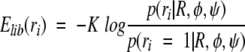(10)

where R is the residue type, and K is a constant, currently set to 3.0 based on optimization of the energy function for a 180-protein test set. The argument of the log is normalized to the highest probability rotamer (defined as r_i = 1), so that the energy of this rotamer is zero and all others are positive. The steric energy function between side-chain atoms and the backbone and between side-chain atoms of different residues is essentially the same as in earlier versions of SCWRL (Bower et al. 1997). This function is a very simple linear repulsive energy term, such that

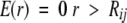(11)

where r is the interatomic distance, and R_ij is the sum of the hard-sphere radii for atoms i and j. Cβ is treated as a backbone atom. The radii used for atoms are as follows: carbon, 1.6 Å; oxygen, 1.3 Å; nitrogen, 1.3 Å; and sulfur, 1.7 Å. The form of the function is designed to represent the repulsive part of the van der Waals energy in a linear form. It is capped at a value of 10.0 kcal/mole to alleviate the fixed rotamer approximation.

Input and output

As with earlier versions of SCWRL, SCWRL3.0 takes a PDB-formatted file that contains backbone coordinates and outputs a file, also in PDB format, containing backbone and predicted side-chain coordinates. Also, SCWRL optionally takes two other files as input. First, a sequence file may be used to change the sequence of the protein. This is an ASCII text file containing only the new sequence. As with earlier versions of SCWRL, this file can be used to instruct SCWRL to preserve the cartesian coordinates of some side chains from the input PDB file by placing them in lower case in the file. These side chains are kept fixed throughout the calculation. Their interaction energies with the rotamers of all other side chains are added to the self-energies of the active side-chain rotamers. In benchmarking tests of homology modeling, keeping conserved residues in their template conformation leads to improved prediction accuracy (data not shown).

Another optional input file for SCWRL contains coordinates for ligands (ions, small molecules, nucleic acids, or proteins) that may interact with side chains to be predicted. These atoms are kept fixed, and are assigned atomic radii based on their atom types. All naturally occurring elements are represented within SCWRL. SCWRL attempts to determine the element from the atom name (see online documentation). Radii were obtained from an analysis of nonbonded ligand-protein atom distances in 5319 proteins in the PDB obtained from the PISCES server (http://dunbrack.fccc.edu/pisces; Wang and Dunbrack 2003). Given the radii for protein atoms (given above), the radii for other atom types, mostly ions, were determined from the minimum distances between ligand atoms of each element type and protein atoms of any type. For example, minimum Zn–O distances in the PDB are ∼1.9 Å. Because the radius of oxygen in SCWRL is 1.3 Å, the radius of Zn is 0.6 Å. Distances were determined such that there would not be significant repulsive interactions in the SCWRL energy function at atom–atom distances observed in the PDB. The radii for 46 elements were determined in this manner. Radii for other elements were arbitrarily set to 1.0 Å.

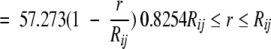
Disulfide bonds

We use an empirically derived scoring function to determine disulfide bond pairings. The function is evaluated for all cysteine pairs in a protein, and a disulfide bond is made if for any rotamers of a given pair, the following scoring function is <45.0,

(12)

where d is the Sγ₁–Sγ₂ distance, A₁ is the bond angle Cβ₁-Sγ₁-Sγ₂, A₂ is the bond angle Sγ₁-Sγ₂-Cβ₂, χ₂ is the dihedral angle Cα₁-Cβ₁-Sγ₁-Sγ₂, χ₄ is the dihedral angle Sγ₁-Sγ₂-Cβ₂-Cα₂, χ₃ is the dihedral angle Cβ₁-Sγ₁-Sγ₂-Cβ₂, and r₁ and r₂ are the rotamers for the first and second cysteines in the proposed disulfide. In a set of 1865 disulfides in 2778 protein structures, this function correctly identifies 1848 of them. It overpredicts 301 disulfides, nearly all of which occur with cysteines that are ligands for ions. In these cases, the disulfide bond function can be turned off with a command line flag (−u).

Implementation details

SCWRL3.0 implementation was done in object-oriented C++. C++ was chosen over other widely used programming languages used in computational biology (FORTRAN, C) because of the high level of abstraction and flexibility it confers. Taking advantage of data encapsulation, inheritance, and polymorphism, the source code uses logical high-level entities (e.g., cluster, biconnected component, residue). At the same time, the code is highly modular, so that changes can be made without affecting the rest of the code. Other advantage are the more error-proof syntax imposed by C++ comparing, for instance, with C, as well as memory allocation/deallocation via wrapper classes instead of the classical C-style memory handling, which is prone to overflows. In terms of design, we preferred an object aggregation approach versus object composition. This provides us with more options regarding future changes and code reusability. We also made extensive use of the Standard Template Library for the parts of the code that involved vectors, sets, stacks, and maps. The development and debugging was done with Microsoft Visual C++ .Net, but the source code was constrained to standard C++ only, in order to keep it cross-compiler and cross-platform compatible. For a C++ compiler for Linux and MacOS X, we used gcc, version 3. SCWRL3.0 has been compiled on Microsoft Windows XP, RedHat Linux 7.3 and 8.0, and MacOS X (version 10.2).

Benchmarking was performed on a dual AMD MP1800+ computer running RedHat Linux 7.3.

Test set

The test set used for speed and accuracy assessments consists of 180 proteins of resolution ≤1.8 Å and mutual sequence identity of <50%, and were obtained from the PISCES server. The chains used were the single-chains in PDB entries 2ilk, 1bec, 1rb9, 1thv, 1pot, 1tca, 2end, 6cel, 1lam, 8abp, 3ebx, 1thg, 2erl, 1pmi, 1kuh, 1ixh, 1c52, 1a7s, 1gci, 1nkd, 1koe, 1ycc, 1tif, 1orc, 2pth, 3grs, 1bs9, 2por, 1l58, 1dcs, 1tag, 3lzt, 1bd8, 1tyv, 1qnf, 1npk, 1mrj, 1eca, 3pte, 1bfd, 7rsa, 1nls, 1a68, 3cyr, 1lcl, 1uae, 2eng, 1a8d, 2acy, 1xnb, 1vqb, 1msi, 1moq, 1hxn, 3vub, 1hfc, 2hbg, 1aqb, 1kid, 1rzl, 1ctf, 1a8e, 1csh, 1pdo, 1smd, 1aba, 2tgi, 1bm8, 2rn2, 2a0b, 1ako, 2ctc, 1b6g, 1msk, 2qwc, 1bfg, 3nul, 1pda, 1arb, 1wab, 1gof, 1bg6, 2cpl, 1vie, 1cor, 1rhs, 1aie, 1bgf, 3cla, 1ifc, 1vjs, 4xis, 1ha1, 1dhn, 1amm, 2sak, 1jer, 1vhh, 1g3p, 1cyo, 1hyp, 1cbn, 3pyp, 1cex, 1ctj, 1a8i, 1mof, 1a6m, 1cnv, 1ryc, 1mrp, 1xjo, 2sn3, 2fdn, 1din, 2baa, 1aru, 1chd, 1cv8, 1bx7, 16pk, 1bdo, 2sns, 3lck, 3seb, 1al3, 1rie, 2dri, 1lbu, 1sbp, 1mml, 1ush, 1edg, 1ads, 2mcm, 1yge, 1whi, 1iab, 1ppn, 1zin, 1lst, 1hka, 1fna, 1poa, 1svy, 3sil, 1fus, 1mun, 1oaa, 1gai, 153l, 1cem, 119l, 1iuz, 1e70, 1mla, 1bj7, 1ezm, 1ra9, 2igd, 1nox, 1fnc, 1aop, 1opd, 2ayh, 1byi, 1cvl, 1ayl, 1axn, 2cba, 1pgs, 5pti, 1bkf, 1vns, 1aho, 1b6a, 1c3d, 1phb, 1rcf, and 1atg.

Availability

SCWRL3.0 is freely available to nonprofit research groups from http://dunbrack.fccc.edu/scwrl3/scwrl3.html. Commercial companies should contact the investigators by electronic mail at RL_Dunbrack@fccc.edu.

Results

As outlined in the Materials and Methods section, the SCWRL3.0 algorithm consists of a number of steps, some in common with earlier versions of SCWRL, some borrowed from other published algorithms, and some novel. We examined each step to determine its effect on reducing the size of the combinatorial problem.

Backtracking algorithm

We use a backtracking algorithm (Kreher and Stinson 1999) to find the minimum-energy combination of rotamers for each biconnected component. Backtracking algorithms are used to generate all feasible solutions to a combinatorial optimization problem by traversing a tree that represents all combinations of the system. This is illustrated in Figure 5 ▶. A number of techniques are available for pruning the tree, so that not all combinations must be enumerated. One of these is to use a bounding function, which is defined at each level of the tree. For the side-chain problem here, we use a bounding function shown in Equation 9 that is the sum of minimum self-energies and minimum pairwise energies for all residues further down in the tree. Another way to improve the pruning is to sort the rotamers of each residue by their self-energies, so that low-energy rotamers are encountered as early in the tree search as possible. It is also possible to sort the residues by their respective number of rotamers. We investigated the effect of these three variants, singly and in combination, and the results are shown in Table 1. In this table, "ener+" and "ener−" indicate sorting of rotamers from lowest-to-highest and highest-to-lowest energy, respectively. Similarly, "nrot+" and "nrot−" indicate sorting the residues from lowest to highest and highest to lowest number of rotamers, respectively. "Bound" means using the bounding function indicated in Equation 9.

Table 1.

Backtracking algorithm comparison

Algorithm	Trial 1	Trial 2	Trial 3	Trial 4	Trial 5	Trial 6
Nrot−, Ener−	415,007	7,074,673	3,591,422	4,856,216	15,209,910	8,610,675
Nrot−	115,799	138,707	30,052	3685	821,949	98,619
Nrot+, Ener−	27,362	119,237	34,396	32,175	42,355	30,904
Nrot−, Ener+	71,629	18,978	477	1932	7255	1487
None	2937	56,130	26,352	8264	42,983	45,055
Nrot+	5363	26,791	2055	3894	9907	9408
Nrot+, Ener+	1684	23,146	730	2201	2681	5321
Bound	906	2481	1360	1112	2692	1123
Nrot+, Ener+, Bound	72	68	70	71	76	62

Number of nodes searched with different sorting conditions and bounding functions (see text). "None" refers to the default SCWRL2.95 algorithm.

In Table 1, the results of six experiments are shown, in which self and pairwise energies were randomly generated for a 10-residue cluster, in which each residue had a random number of rotamers between 2 and 10. In all cases studied, each variation identified the same lowest-energy configuration. The results indicate that sorting residues by number of rotamers (nrot+), sorting rotamers by self-energies (ener+), and using the bounding function (bound) each has a significant effect. In combination, they are very powerful, reducing the number of nodes searched from ≥50,000 to <100. With random energies, the number of nodes can be pushed to ≥200 and still be solved in less than a minute (data not shown). With the energy function used currently in SCWRL in which many pairwise energies are zero, the algorithm is not as powerful because the bounding function sometimes does not change from level to level. However, breaking the degeneracy with favorable packing and electrostatic interactions will allow the branch-and-bound algorithm greater efficiency in solving larger clusters.

Computational complexity

SCWRL3.0 uses an updated version of the backbone-dependent rotamer library (Dunbrack and Cohen 1997; Dunbrack 2002), with improved Bayesian analysis of the probabilities and mean and variance of dihedral angles at all values of φ and ψ. The backbone-dependent rotamer library contains information on all rotamer types for each side chain. For instance, lysine has four dihedral angle degrees of freedom, each of which can take on one of three different rotamer values, for a total of 81 rotamers. However, many of these are sterically impossible and have never or only very rarely been seen in the PDB. Because the library contains many rotamers of very low probability, SCWRL reads in the rotamers from highest to lowest probability, given the backbone conformation, and keeps only the top D proportion of the cumulative density. Currently D = 0.9 is used, because the prediction rate does not improve with higher values of D (M.J. Bower, unpubl.). After the coordinates are constructed for the input rotamers, the DEE step with the simple Goldstein criterion (Goldstein 1994) is used to remove rotamers that cannot be part of the global minimum-energy configuration. In Table 2, we list the average number of rotamers that fall within the top 90% of density for each side-chain type, as well as the number that pass the DEE step. For Lys and Arg, the number of rotamers is reduced from 81 to less than 2 on average by the top-D and DEE criteria. However, the range is quite broad due to the variability in side-chain environments (buried, surface, number of near neighbors).

Table 2.

Average number of rotamers in the top 90% of density in the rotamer library and after dead-end elimination

Residue type	No. of rotamers in library	No. of top-D rotamers	σ	No. of DEE rotamers	σ
ARG	81	21.2	3.7	2.0	2.2
ASN	18	6.9	1.0	1.3	0.7
ASP	6	4.3	0.8	1.2	0.6
CYS	3	2.1	0.4	1.1	0.3
GLN	36	12.0	2.5	1.4	1.2
GLU	27	11.2	1.0	1.4	1.2
HIS	9	4.8	0.9	1.4	0.9
ILE	9	2.4	0.9	1.2	0.4
LEU	9	2.0	0.6	1.1	0.4
LYS	81	17.1	3.1	1.3	1.2
MET	27	8.9	1.3	1.9	1.5
PHE	6	2.6	0.6	1.3	0.6
PRO	2	1.9	0.3	1.0	0.2
SER	3	2.4	0.5	1.1	0.3
THR	3	1.6	0.6	1.1	0.2
TRP	9	4.7	0.8	1.7	1.0
TYR	6	2.5	0.7	1.3	0.5
VAL	3	1.5	0.7	1.0	0.2

Top-D indicates top 90% of density; DEE, dead-end elimination.

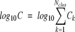
We can measure the complexity of the side-chain problem by calculating the log₁₀ of the number of viable combinations at each stage of the calculation. In Figure 6, A and B ▶, the log₁₀ combinations for the top-D rotamers and the post-DEE rotamers, respectively, are shown for the 180-protein test set versus the length of each protein. These values are calculated from the equation

(13)

where n_i is the number of viable rotamers for residue i. The log-top-D rotamer complexities are essentially linear in the number of residues. The DEE step reduces the complexity from ∼150 log₁₀ units for 300-residue proteins to 10 to 30 log₁₀ units.

Figure 6.

Complexity of combinatorial problem at various stages of calculation. Complexity is represented as log₁₀ of the number of combinations that would have to be searched at each stage, if subsequent stages were not performed. Test set of 180 proteins was used. (A) Log₁₀ of combinations of top 90% rotamers. (B) Log₁₀ of combinations of post-DEE rotamers. (C) Log₁₀ of sum of cluster combinations. (D) Log₁₀ of sum of biconnected component combinations. (E) Log₁₀ of total number of nodes in backtracking trees searched

After the DEE step, SCWRL converts the side-chain problem into a graph containing residues as vertices and interactions between residues as edges. An edge occurs between residues i and j if for some rotamers r_i and r_j there is an energy E_pair(r_i,r_j) ≠ 0. This graph is generally not connected but rather will comprise several smaller internally connected graphs, which do not have edges between them. The minimum-energy configuration of each of these connected subgraphs is part of the global minimum energy configuration of the entire system. Determining these subgraphs reduces the complexity of the problem from that of the total graph to that of the sum over the subgraphs. We refer to these connected subgraphs as clusters. In Figure 7 ▶, we show a histogram of the cluster sizes in the 180-protein test set. In this figure, clusters of size 1 are omitted. Of 34,342 non-Ala, non-Gly residues, only 4996 of them exist in clusters of more than one residue. Nearly all clusters are size ≤40, with one cluster in the 180-protein set of 78 residues. Once the clusters are determined, the complexity of the problem is reduced to a sum over the clusters,

Figure 7.

Cluster sizes in 180 proteins. Size of graphs after DEE step is performed and edges among residue vertices are determined. Clusters of size 1 are not shown.

(14)

where C_k is the complexity for each cluster k, and C is the total complexity of the problem. The results are shown in Figure 6C ▶.

Some clusters could be solved immediately by the backtracking algorithm, but many of them are still too large to be enumerated in a reasonable amount of time, as demonstrated by Figure 6C ▶. A novel step in SCWRL3.0 is to break up the cluster graphs into biconnected components, which can be solved separately for each articulation point and then combined to produce a global minimum energy configuration for the cluster. The success of the method depends on the size of these biconnected components and on whether they can be solved quickly. A histogram of the biconnected component sizes is shown in Figure 8 ▶. Most biconnected components have sizes of 2 or 3 residues, although a small number are as large as 20 residues. The complexity of the problem is now reduced to a sum over the biconnected components, as shown in Figure 6D ▶. Even the most complex protein now has complexity of <10¹¹. Finally, the backtracking algorithm solves each biconnected component without fully enumerating all of the combinations. The complexity is then the number of combinations actually evaluated by the backtracking algorithm. This is shown in Figure 6E ▶, in which the maximum number of combinations actually evaluated is <10⁷.

Figure 8.

Biconnected component sizes in 180 proteins. The number of biconnected components of size 1 is 2325 (truncated on the graph to show the distribution at higher sizes).

Although the DEE step is effective in reducing the complexity, it is not sufficient on its own to reduce the problem to manageable size for most proteins, either with or without the clustering step. However, the number of combinations after breaking the clusters into biconnected components is easily solved for each protein. The branch-and-bound algorithm is very efficient in solving the biconnected components, although its impact on the total size of the problem is small. However, as noted previously, if we add flexibility to the side chains and increase the number of interactions between residues, the branch-and-bound algorithm is likely to be very useful in keeping the calculation time to a minimum.

Speed

Previous versions of SCWRL were generally very fast compared with other side-chain prediction programs, but suffered from two drawbacks. One is that a number of heuristics were used to reduce the complexity by removing rotamers with backbone energies >5.0 kcal/mole (parameter EBBMAX) and ignoring pairwise interactions <10.0 kcal/mole when determining the residue graph (parameter EPAIRMIN). Varying these parameters by increasing EBBMAX and reducing EPAIRMIN in SCWRL2.95 increases the complexity and computation time of the problem rapidly. The other is that for a small number of proteins SCWRL would get stuck trying to solve very large clusters and, in fact, would never reach a solution. In Table 3, we compare the computational times for SCWRL2.95 and SCWRL3.0 with various settings of EBBMAX and EPAIRMIN. Although SCWRL2.95 solves the 180-protein test set in 17 min with the previous default settings, as these parameters are varied so that more rotamers and rotamer pairs are included in the calculation, the time increases rapidly. The number of proteins that can each be solved in ≤15 min of CPU time (for each protein) also decreases. We implemented EBBMAX and EPAIRMIN in SCWRL3.0 for purposes of comparison with SCWRL2.95. When these parameters are omitted (equivalent of EBBMAX of infinity and EPAIRMIN of 0.0), the time taken for SCWRL3.0 on the test set is 13 min. Even with EBBMAX of 50.0, SCWRL2.95 is only able to complete 132 proteins in 4.3 h. This time does not include the failures. We have set the default value of EBBMAX to 50.0 and EPAIRMIN to infinity (i.e., no minimum energy cutoff for pairs of rotamers) in SCWRL3.0.

Table 3.

Speed of SCWRL2.95 and SCWRL3.0 calculations on the 180-protein test set

		SCWRL2.95		SCWRL3.0
EBBMAX	EPAIRMIN	Time (sec)	No. completed	Time (sec)	No. completed
5	10	1012a	180	234	180
5	0	3430	174	228	180
50	10	8549	168	395	180
50	0	15,537	132	404a	180
∞	0	N.D.	N.D.	790	180

EBBMAX is the maximum backbone/side-chain interaction energy for a rotamer to be included in the calculations. EPAIRMIN is the minimum side-chain/side-chain interaction energy for two residues to be considered connected in determining clusters of interacting residues.

Each calculation was stopped if it took >15 min (900 sec). Time does not include the failures. Number completed is out of 180 proteins. N.D. indicates not done.

^a Default parameters for each program.

We also compared SCWRL3.0 with the generalized DEE algorithm of Looger and Hellinga (2001). These investigators present CPU time for several large proteins, including 1xwl (580 residues) 1bu7 (910 residues), 1a8i (812 residues), and 1b0p (2462 residues). For these same proteins, their times were 1823, 2472, 2590, and 3018 sec, respectively, on an SGI R12000 processor. SCWRL3.0 achieves times of 17, 43, 86, and 239 sec, respectively, on an Athlon MP1800+ processor. The AMD CPU is 1.3 to 1.8 times faster than the SGI R12000 (depending on the clock speed of the SGI CPU; see http://www.specbench.org/osg/cpu2000/results/cpu2000.html#SPECfp), which makes SCWRL at a minimum 7 (1b0p at 1.8×) and maximum 82 times (1xwl at 1.3×) faster on these four proteins.

Accuracy

We used the same set of 180 proteins to determine the prediction accuracy of SCWRL3.0 and to compare this accuracy to SCWRL2.95, the most recent, publicly released version of SCWRL. Although the energy function is essentially identical to that of SCWRL2.95, SCWRL3.0 uses a new rotamer library and is able to perform a search including all interactions in the energy function. These differences result in slightly higher prediction accuracy. Table 4 lists the χ₁ and χ₂ accuracy (within 40°) of each residue type achieved by the backbone-dependent rotamer library alone, SCWRL2.95, and SCWRL3.0. Using only the most preferred rotamer from the backbone-dependent rotamer library results in 73.0% χ₁ accuracy. The accuracy for SCWRL3.0 is 82.6% for χ₁ and 73.7% for χ₁₊₂ which are slightly higher than the results for SCWRL2.95 of 81.7% and 70.9%, respectively. Further analysis of prediction accuracy is outside the scope of this article, and will be considered when new energy functions are implemented.

Table 4.

Accuracy results for backbone-dependent rotamer library alone (BBDEP), SCWRL2.95, and SCWRL3.0 in 180-protein test set

		χ1 Prediction accuracy			χ1+2 Prediction accuracy
Residue type	No. of residues	BBDEP	SCWRL2.95	SCWRL3.0	BBDEP	SCWRL2.95	SCWRL3.0
PHE	1653	75.4	92.9	93.7	68.3	84.9	87.4
TYR	1633	74.1	91.0	92.3	68.9	83.8	86.5
ILE	2134	87.7	91.8	91.8	70.1	78.1	80.4
LEU	3406	72.9	89.0	89.9	66.1	80.1	81.8
VAL	2787	85.9	89.3	89.9	85.9	89.3	89.9
TRP	671	68.4	87.0	88.4	41.3	60.6	64.8
CYS	679	80.6	86.5	88.2	80.6	86.5	88.2
THR	2449	85.0	87.4	88.0	85.0	87.4	88.0
HIS	899	67.7	83.3	85.3	59.3	66.4	75.1
PRO	1994	82.6	83.9	84.4	82.6	83.9	84.4
ASP	2493	71.7	80.2	80.8	62.6	56.5	70.4
MET	789	64.9	76.9	80.4	37.8	59.8	65.1
ASN	2036	68.1	77.9	78.7	55.6	56.9	66.1
ARG	1888	62.6	75.8	76.9	48.7	61.9	63.7
GLN	1569	66.1	74.0	74.6	40.9	54.7	52.6
LYS	2319	66.5	73.9	74.0	46.8	57.0	57.0
GLU	2267	61.7	70.0	71.3	39.9	50.5	51.7
SER	2676	62.6	65.7	66.4	62.6	65.7	66.4
All	34,342	73.0	81.7	82.6	63.2	70.9	73.7

χ₁ prediction accuracy is expressed as percent of side chains with χ₁ dihedral angles within 40 degrees of the X-ray crystallographic value. For side chains with only χ₁, the χ₁ accuracy is given in the χ₁₊₂ columns. For χ₁₊₂ to be correct, both χ₁ and χ₂ must be within 40 degrees of their X-ray values. Residue types are sorted by their SCWRL3.0 χ₁ accuracy.

Discussion

As the number of protein families with at least one structure is rising rapidly, the need for fast and accurate homology modeling is increasing. Improving the accuracy will require more complex energy functions (Liang and Grishin 2002) and flexibility of side chains around rotamer dihedral angle values and standard bond lengths and angles (Mendes et al. 1999a,b; Xiang and Honig 2001). The new algorithm is robust enough to handle energy functions and conformational flexibility that increase the connectedness of side-chain interaction graphs. In the future, we plan to implement favorable packing interactions, hydrogen bonds, electrostatics, and solvation terms to improve side-chain prediction accuracy. Allowing for flexibility of side chains away from standard bond lengths and angles or fixed dihedral angles for each rotamer will also be tested for improved accuracy. Nevertheless, the current energy function and algorithm produce predictions that are better than nearly all published methods that are publicly available (G. Wang and R.L. Dunbrack, unpubl.), except some that are two to three orders of magnitude slower (Mendes et al. 2001b; Liang and Grishin 2002).

SCWRL has enjoyed widespread use in the protein structure prediction community because of its ease-of-use, accuracy, and speed. In CASP5, SCWRL was used by at least 12 groups for side-chain prediction (see http://www.forcasp.org). Of the top 10 groups in side-chain prediction on high sequence-identity targets, SCWRL was used by 5 of them, and the backbone-dependent rotamer library used in SCWRL was used by 2 other groups (see http://forcasp.org/modules.php?name=Papers&file=article&sid=1985). SCWRL is designed to be used as a homology-modeling tool, and so it preserves all input coordinate features (e.g., residue numbering, chain IDs, ligand atom positions), in contrast to many publicly available programs. We have designed SCWRL3.0 to retain these advantages, and at the same time to provide for increased speed and reliability and future opportunities for increased accuracy through new energy functions and flexibility.

References

- Berman, H.M., Westbrook, J., Feng, Z., Gilliland, G., Bhat, T.N., Weissig, H., Shindyalov, I.N., and Bourne, P.E. 2000. The Protein Data Bank. Nucleic Acids Res. 28 235–242. [DOI] [PMC free article] [PubMed] [Google Scholar]
- Bower, M.J., Cohen, F.E., and Dunbrack Jr., R.L. 1997. Prediction of protein side-chain rotamers from a backbone-dependent rotamer library: A new homology modeling tool. J. Mol. Biol. 267 1268–1282. [DOI] [PubMed] [Google Scholar]
- Dahiyat, B.I. and Mayo, S.L. 1996. Protein design automation. Protein Sci. 5 895–903. [DOI] [PMC free article] [PubMed] [Google Scholar]
- De Maeyer, M., Desmet, J., and Lasters, I. 1997. All in one: A highly detailed rotamer library improves both accuracy and speed in the modelling of side-chains by dead-end elimination. Fold Des. 2 53–66. [DOI] [PubMed] [Google Scholar]
- ———. 2000. The dead-end elimination theorem: Mathematical aspects, implementation, optimizations, evaluation, and performance. Methods Mol. Biol. 143 265–304. [DOI] [PubMed] [Google Scholar]
- Desjarlais, J.R. and Handel, T.M. 1995. De novo design of the hydrophobic cores of proteins. Protein Sci. 4 2006–2018. [DOI] [PMC free article] [PubMed] [Google Scholar]
- Desmet, J., De Maeyer, M., Hazes, B., and Lasters, I. 1992. The dead-end elimination theorem and its use in protein side-chain positioning. Nature 356 539–542. [DOI] [PubMed] [Google Scholar]
- Desmet, J., De Maeyer, M., and Lasters, I. 1997. Theoretical and algorithmical optimization of the dead-end elimination theorem. Pac. Symp. Biocomput. 1997 122–133. [PubMed] [Google Scholar]
- Desmet, J., Spriet, J., and Lasters, I. 2002. Fast and accurate side-chain topology and energy refinement (FASTER) as a new method for protein structure optimization. Proteins 48 31–43. [DOI] [PubMed] [Google Scholar]
- Dunbrack Jr., R.L. 1999. Comparative modeling of CASP3 targets using PSI-BLAST and SCWRL. Proteins 3 81–87. [DOI] [PubMed] [Google Scholar]
- ———. 2002. Rotamer libraries in the 21st century. Curr. Opin. Struct. Biol. 12 431–440. [DOI] [PubMed] [Google Scholar]
- Dunbrack Jr., R.L. and Cohen, F.E. 1997. Bayesian statistical analysis of protein side-chain rotamer preferences. Protein Sci. 6 1661–1681. [DOI] [PMC free article] [PubMed] [Google Scholar]
- Dunbrack Jr., R.L. and Karplus, M. 1993. Backbone-dependent rotamer library for proteins: Application to side-chain prediction. J. Mol. Biol. 230 543–574. [DOI] [PubMed] [Google Scholar]
- ———. 1994. Conformational analysis of the backbone-dependent rotamer preferences of protein sidechains. Nature Struct. Biol. 1 334–340. [DOI] [PubMed] [Google Scholar]
- Goldstein, R.F. 1994. Efficient rotamer elimination applied to protein side-chains and related spin glasses. Biophys. J. 66 1335–1340. [DOI] [PMC free article] [PubMed] [Google Scholar]
- Gordon, D.B. and Mayo, S.L. 1999. Branch-and-terminate: A combinatorial optimization algorithm for protein design. Structure Fold Des. 7 1089–1098. [DOI] [PubMed] [Google Scholar]
- Holm, L. and Sander, C. 1991. Database algorithm for generating protein backbone and sidechain coordinates from a Ca trace: Application to model building and detection of coordinate errors. J. Mol. Biol. 218 183–194. [DOI] [PubMed] [Google Scholar]
- Hwang, J.K. and Liao, W.F. 1995. Side-chain prediction by neural networks and simulated annealing optimization. Protein Eng. 8 363–370. [DOI] [PubMed] [Google Scholar]
- Keller, D.A., Shibata, M., Marcus, E., Ornstein, R.L., and Rein, R. 1995. Finding the global minimum: A fuzzy end elimination implementation. Protein Eng. 8 893–904. [DOI] [PubMed] [Google Scholar]
- Kelley, L.A., MacCallum, R.M., and Sternberg, M.J. 2000. Enhanced genome annotation using structural profiles in the program 3D-PSSM. J. Mol. Biol. 299 499–520. [DOI] [PubMed] [Google Scholar]
- Koehl, P. and Delarue, M. 1995. A self consistent mean field approach to simultaneous gap closure and side-chain positioning in homology modeling. Nat. Struct. Biol. 2 163–170. [DOI] [PubMed] [Google Scholar]
- Kono, H. and Doi, J. 1994. Energy minimization method using automata network for sequence and side-chain conformation prediction from given backbone geometry. Proteins 19 244–255. [DOI] [PubMed] [Google Scholar]
- Kreher, D.L. and Stinson, D.R. 1999. Combinatorial algorithms: Generation, enumeration, and search. CRC Press, Boca Raton, FL.
- Lasters, I. and Desmet, J. 1993. The fuzzy-end elimination theorem: Correctly implementing the side-chain placement algorithm based on the dead-end elimination theorem. Protein Eng. 6 717–722. [DOI] [PubMed] [Google Scholar]
- Lasters, I., DeMaeyer, M., and Desmet, J. 1995. Enhanced dead-end elimination in the search for the global minimum energy conformation of a collection of protein side-chains. Protein Eng. 8 815–822. [DOI] [PubMed] [Google Scholar]
- Laughton, C.A. 1994. Prediction of protein side-chain conformations from local three-dimensional homology relationships. J. Mol. Biol. 235 1088–1097. [DOI] [PubMed] [Google Scholar]
- Lee, C. and Subbiah, S. 1991. Prediction of protein side-chain conformation by packing optimization. J. Mol. Biol. 217 373–388. [DOI] [PubMed] [Google Scholar]
- Liang, S. and Grishin, N.V. 2002. Side-chain modeling with an optimized scoring function. Protein Sci. 11 322–331. [DOI] [PMC free article] [PubMed] [Google Scholar]
- Looger, L.L. and Hellinga, H.W. 2001. Generalized dead-end elimination algorithms make large-scale protein side-chain structure prediction tractable: Implications for protein design and structural genomics. J. Mol. Biol. 307 429–445. [DOI] [PubMed] [Google Scholar]
- Lovell, S.C., Word, J.M., Richardson, J.S., and Richardson, D.C. 2000. The penultimate rotamer library. Proteins 40 389–408. [PubMed] [Google Scholar]
- McGregor, M.J., Islam, S.A., and Sternberg, M.J.E. 1987. Analysis of the relationship between side-chain conformation and secondary structure in globular proteins. J. Mol. Biol. 198 295–310. [DOI] [PubMed] [Google Scholar]
- Mendes, J., Baptista, A.M., Carrondo, M.A., and Soares, C.M. 1999a. Improved modeling of side-chains in proteins with rotamer-based methods: A flexible rotamer model. Proteins 37 530–543. [DOI] [PubMed] [Google Scholar]
- Mendes, J., Soares, C.M., and Carrondo, M.A. 1999b. Improvement of side-chain modeling in proteins with the self-consistent mean field theory method based on an analysis of the factors influencing prediction. Biopolymers 50 111–131. [DOI] [PubMed] [Google Scholar]
- Mendes, J., Baptista, A.M., Carrondo, M.A., and Soares, C.M. 2001a. Implicit solvation in the self-consistent mean field theory method: Side-chain modeling and prediction of folding free energies of protein mutants. J. Comp. Aided. Mol. Design 15 721–740. [DOI] [PubMed] [Google Scholar]
- Mendes, J., Nagarajaram, H.A., Soares, C.M., Blundell, T.L., and Carrondo, M.A. 2001b. Incorporating knowledge-based biases into an energy-based side-chain modeling method: Application to comparative modeling of protein structure. Biopolymers 59 72–86. [DOI] [PubMed] [Google Scholar]
- Pierce, N.A., Spriet, J.A., Desmet, J., and Mayo, S.L. 1999. Conformational splitting: A more powerful criterion for dead-end elimination. J. Comp. Chem. 21 999–1009. [Google Scholar]
- Ponder, J.W. and Richards, F.M. 1987. Tertiary templates for proteins: Use of packing criteria in the enumeration of allowed sequences for different structural classes. J. Mol. Biol. 193 775–792. [DOI] [PubMed] [Google Scholar]
- Samudrala, R. and Moult, J. 1998. Determinants of side chain conformational preferences in protein structures. Protein Eng. 11 991–997. [DOI] [PubMed] [Google Scholar]
- Summers, N.L. and Karplus, M. 1989. Construction of side-chains in homology modelling: Application to the C-terminal lobe of rhizopuspepsin. J. Mol. Biol. 210 785–811. [DOI] [PubMed] [Google Scholar]
- Tarjan, R. 1972. Depth first search and linear graph algorithms. SIAM J. Comput. 1 146–160. [Google Scholar]
- Tuffery, P., Etchebest, C., Hazout, S., and Lavery, R. 1991. A new approach to the rapid determination of protein side chain conformations. J. Biomol. Struct. Dyn. 8 1267–1289. [DOI] [PubMed] [Google Scholar]
- Voigt, C.A., Gordon, D.B., and Mayo, S.L. 2000. Trading accuracy for speed: A quantitative comparison of search algorithms in protein sequence design. J. Mol. Biol. 299 789–803. [DOI] [PubMed] [Google Scholar]
- Wang, G. and Dunbrack Jr., R.L. 2003. PISCES: A protein sequence culling server. Bioinformatics (in press). [DOI] [PubMed]
- Wilson, C., Gregoret, L., and Agard, D. 1993. Modeling side-chain conformation for homologous proteins using an energy-based rotamer search. J. Mol. Biol. 229 996–1006. [DOI] [PubMed] [Google Scholar]
- Word, J.M., Lovell, S.C., LaBean, T.H., Taylor, H.C., Zalis, M.E., Presley, B.K., Richardson, J.S., and Richardson, D.C. 1999a. Visualizing and quantifying molecular goodness-of-fit: Small-probe contact dots with explicit hydrogen atoms. J. Mol. Biol. 285 1711–1733. [DOI] [PubMed] [Google Scholar]
- Word, J.M., Lovell, S.C., Richardson, J.S., and Richardson, D.C. 1999b. Asparagine and glutamine: Using hydrogen atom contacts in the choice of side-chain amide orientation. J. Mol. Biol. 285 1735–1747. [DOI] [PubMed] [Google Scholar]
- Xiang, Z. and Honig, B. 2001. Extending the accuracy limits of prediction for side-chain conformations. J. Mol. Biol. 311 421–430. [DOI] [PubMed] [Google Scholar]