The problem of the spreading of a liquid film along a solid surface: A new mathematical formulation

Abstract

A new mathematical model is proposed for the spreading of a liquid film on a solid surface. The model is based on the standard lubrication approximation for gently sloping films (with the no-slip condition for the fluid at the solid surface) in the major part of the film where it is not too thin. In the remaining and relatively small regions near the contact lines it is assumed that the so-called autonomy principle holds—i.e., given the material components, the external conditions, and the velocity of the contact lines along the surface, the behavior of the fluid is identical for all films. The resulting mathematical model is formulated as a free boundary problem for the classical fourth-order equation for the film thickness. A class of self-similar solutions to this free boundary problem is considered.

Section 1. Introduction

The problem of the spreading of a liquid film along a solid surface is nowadays widely known and attracts the attention of physicists, fluid mechanicians, and applied mathematicians (see refs. 1–13, where further references can be found). After the pioneering work of Bernis and Friedman (14) it has attracted a continuously growing amount of mathematical research (see refs. 15–24, where further references can be found; R. Kersner and A. Shishkov, F. Otto, and J. Hulshof and A. Shishkov, personal communications). A sketch of the phenomenon is shown in Fig. 1 (for simplification we assume symmetry of the film and a one-dimensional film flow).

Figure 1.

The thin film flow: A schematic representation. 1, Solid surface; 2, liquid film; and 3, gas.

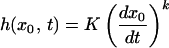
The basic equation for the film thickness h(x, t), due to Greenspan (1), is

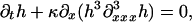1.1

where t is the time, x is the spatial coordinate, κ = 2γ/μ is a constant, γ is the surface tension, and μ is the viscosity of the liquid. Eq. 1.1 is derived on the basis of two assumptions: The first assumption is the applicability of the lubrication approximation (see ref. 25) to film flow. However, this assumption is valid for gently sloping flows only, for which ∂_xh is small and the vertical component of the velocity is negligible.

The second assumption is that the hydrodynamic pressure p is created entirely by the surface tension γ and the Laplace formula is valid, according to which p = −2γk, wherein the lubrication approximation curvature is equal to k = ∂_xx²h. The boundaries x = ±x₀(t) are the free boundaries of the boundary value problem for 1.1—i.e., they are not prescribed beforehand, and should be determined in the course of solution.

Since the partial differential equation 1.1 is of fourth order, at each of the two boundaries x = ±x₀(t) three conditions are expected to be needed to determine uniquely the evolution of the fluid film: apart from the two seemingly natural conditions (h = 0 and vanishing flux), an empirical condition is usually proposed which relates the velocities ±x′₀(t) of the free boundaries to the film slope ∂_xh, and which in the case of complete wetting is believed to reduce to the condition of zero slope.

The main difficulty of the lubrication theory of thin films is the following: If we assume that the lubrication approximation is valid up to the contact lines x = ±x₀(t)—i.e., if we assume that Eq. 1.1 holds at all points (x, t) satisfying |x| ≤ x₀(t)—then it follows, for example from a straightforward asymptotic expansion near the contact line, that the film should be nonexpanding. In other words, the function x₀(t) is nonincreasing and an infinite energy is needed for expansion of the spatial support of the film.

The usual approach to overcome this problem is the introduction of an “effective slip” of the fluid film at the solid surface (see ref. 12 for further references to the literature) which leads to an equation of the type 1.1 with the factor h³ replaced by h³ + βh², where β is an empirical small positive parameter often referred to as “effective slip parameter.” The dimension of β is that of length, and to obtain the qualitative agreement with experiments it should be small in comparison to the typical thickness of the film.

In this paper we propose an entirely different approach, without introducing the concept of effective slip. Its essence is as follows. It is not reasonable to assume that the lubrication approximation is valid up to the contour lines of the film. Therefore we divide the region occupied by the film into two or possibly three regions: the basic region, where the basic assumptions leading to Eq. 1.1 are valid; the contour region near the contour lines of the film, where the film is not necessarily gently sloping and where the Laplace formula is not valid due to nonequilibrium character of the distribution of the cohesive forces; and possibly a precursor region, which could exist ahead of the contour line [see de Gennes (10), where further references can be found).

Our two basic assumptions are the following:

(i)  The autonomy principle: For given material components (gas, liquid, and solid), given external conditions such as temperature and pressure, and given the velocity of propagation V = dx₀/dt of the contact line along the surface, the structure of the contour region is autonomous—i.e., the slope of the film and the distribution of the forces inside the contour region are identical for all films, independent of their size, time of extension, etc.

(ii)  The smallness condition: The longitudinal size of the contour region is small in comparison to the size of the basic region.

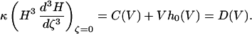
These mathematical assumptions correspond to the physical concept of strong short-range cohesive forces [see the excellent review by Dzyaloshinski et al. (26)] localized in a small region near the contact lines. In Section 2 we shall show that they lead to the following free boundary problem for h(x, t): The basic equation 1.1 holds in the basic region, while at an interface x = x₀(t) which separates the basic and contour regions, the three free boundary conditions hold:

1.2

where h₀(V), G(V), and C(V) are given functions of the velocity of propagation V determined by the nature of the materials and by the external conditions. We emphasize that here we shall use only “minimal” assumptions in the derivation of 1.2 in the sense that only further investigations and comparisons with the experiments can shed light on the nature of the functions h₀(V), G(V), and C(V). We consider the present paper to be basically an introduction of a new concept to describe advancing fronts: V = dx₀/dt > 0. To develop a more complete model one should incorporate such phenomena as film rupture and the disappearance of dry spots (in the one-dimensional formulation this corresponds to advancing fronts which meet each other).

In this paper we derive the free boundary conditions 1.2, analyze some special cases of them, and demonstrate that a natural mathematical approach to reduce the problem to the limiting case h₀ = 0, and, to deal with the singularities at the contour lines, used for instance in the mathematical theory of cracks (27, 28), does not work here. This is shown by using a complete description of the local traveling wave solutions to Eq. 1.1.

Section 2. The Physical Model of the Triple Contact Region

At the contour line there is contact of three phases: fluid, solid, and ambient gas. To derive the boundary conditions at the contour lines we propose to use the micromechanical approach based upon the explicit introduction of the cohesive forces and upon the principle of the “autonomy of the triple contact region” around the contour lines.

We note, first of all, that the basic hypotheses used in the derivation of Eq. 1.1, that of the lubrication approximation—i.e., of gently sloping flows—and that of fluid pressure created by the surface tension only, are not valid everywhere in the film. Near the contour lines the slope could be large, the height of the film is small, and the distribution of the cohesive forces does not allow the use of the simple Laplace formula. Therefore let us divide the film—i.e., the region occupied by the fluid (Fig. 1)—into three parts: (i) the basic region, where the basic assumptions leading to Eq. 1.1 are valid; (ii) the contour region near the contour lines, where the flow is not necessarily gently sloping, the lubrication approximation is invalid, and the distribution of the cohesive forces does not allow use of the simple Laplace formula; and (iii) the precursor region, which, according to de Gennes (ref. 10, where the previous sources are also referenced), does exist under certain circumstances ahead of the contact line (Fig. 2).

Figure 2.

The “autonomous” region near the contour line. 1, Basic region where Eq. 1.1 is valid; 2, autonomous contour region; and 3, precursor.

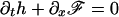
The relationship for the flux in the contour region becomes:

2.1

where ℱ is a certain function matching the ordinary expression κh³∂_xxx³h at the boundary between the contour region and the basic region.

Now we introduce the basic assumptions (cf. refs. 27 and 28):

(i) The Autonomy Principle. For given materials: fluid, gas, and solid surface, given external conditions: temperature and pressure, and a given velocity V of propagation of the contact line along the surface, the structure of the contour region is autonomous—i.e., the slope of the film and the distribution of forces inside the contour region is identical for all films, independent of their size, time of extension, etc. All these circumstances can influence the extension rate of the boundary, but when it is fixed, the structure is identical for all films.

(ii) The Smallness Condition. The longitudinal size d of the contour region is small in comparison with the size of the basic region.

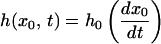
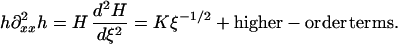
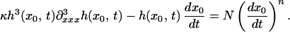
According to the equation of mass balance and 2.1, the equation governing the film height h takes the form

2.2

valid in both the basic and the contour regions. The usual asymptotic technique (29, 30) leads to a solution of traveling-wave type

2.3

which is being established in the vicinity of the contour lines in times of the order of d/V—i.e., instantaneously in the time scale of the film extension, x₀/V, V = dx₀/dt. Putting 2.3 into Eq. 2.2, we obtain

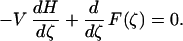2.4

After an integration of 2.4 we obtain

2.5

Here C(V) is an integration constant; generally speaking it can depend on the velocity of the contact line propagation dx₀/dt = V. Moreover, due to the autonomy of the contour region, C(V) is a universal function, identical for given external conditions for all films and for a given triplet: fluid–gas–solid surface.

According to the definition of the autonomous contour region the following relations should hold at its internal boundary x = x₀(t), ζ = 0:

2.6

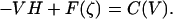
where h₀(V) is again a function of the spreading velocity. According to our assumptions this function is identical for all films under given external conditions and a given triplet. Due to 2.5 and 2.6 the following relation is obtained

2.7

Again, D(V) is a universal function for all films under given external conditions and a given triplet.

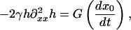
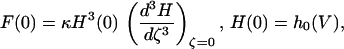
Let us turn now to the momentum balance of the contour region. The force acting from the side of the basic region on the contour region is equal to the extra fluid pressure at ζ = 0, p(0), times the height h₀(V) of the film at ζ = 0. It is equal to the tangential force, acting on the contour region from the solid surface (and, perhaps, also from the film precursor). Due to the autonomy, this tangential force is also a universal function of the velocity V: G(V). However, at the boundary between the basic region and the contour region the pressure is continuous, the lubrication approximation and the Laplace formula are valid, and therefore

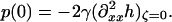2.8

Thus the condition of equilibrium assumes the form

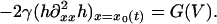2.9

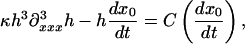
Summarizing, we obtain the conditions at the contour line ζ = 0, x = x₀(t) in the form 1.2. Unfortunately (see the next section), the natural procedure of the passage to the limit h₀ → 0 does not work directly. There are several different, more special, proposals concerning this model which can be discussed. Among them is keeping h₀(V) different from zero and neglecting the flux outside the contour region as well as the tangential force acting on the small contour region. In this case the boundary conditions at the moving boundary x₀(t) take the specially instructive form

2.13

2.14

2.15

Section 3. Impossibility of Simplifying the Boundary Conditions

Since h₀(V) is small in comparison with the film thickness h(x, t) in the basic region where the lubrication approximation is valid, it seems natural to simplify the problem in the following way. Consider the limiting procedure h₀(V) → 0 and try to find a singular solution to Eq. 1.1 with a coefficient at the singularity that depends on the velocity V. In fact, such a limiting procedure is traditional in the theory of cracks (see refs. 27 and 28). In particular, this singular solution should have a nonzero flux at the contour line (zero flux, as was mentioned in Introduction, would lead to a nonexpanding film). However, this procedure does not lead to a successful result. To show this, let us consider the local situation near the left contact line x = −x₀(t). This situation is described by the fast establishing traveling wave solution

3.1

Then Eq. 1.1 leads to the relation

3.2

According to our assumptions, we set

3.3

Integrating 3.2 and using conditions 3.3, we obtain the traveling wave problem

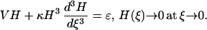3.4

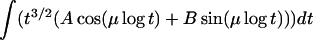
It can be proved (see below) that for ɛ > 0 any solution to the problem 3.4 has the following asymptotic behavior at ξ → 0

3.5

where C is a fixed constant which does not depend on the velocity. If ɛ < 0 the problem 3.4 does not possess positive solutions. The expansion 3.5 leads to an unphysical situation: the force acting on the contour region which, according to the previous section, is proportional to h∂_xx²h, is infinite at the edge of the fluid. Indeed, according to 3.5 at ξ → 0

3.6

This result means that for our free boundary problem the mathematical limiting procedure h₀(V) → 0 is expected to fail.

The asymptotic expansion 3.5 follows at once from the following, more precise statement:

(i)  For ɛ > 0, if H(ξ) is a smooth and positive solution to the problem 3.4, there exist constants A and B such that as ξ → 0⁺,

3.7

where

3.8

are absolute constants.

(ii)  For any ɛ > 0 and for any real numbers A, B there exists a region 0 ≤ ξ < ξ₀ where the problem 3.4 has a uniquely determined smooth and positive solution H(ξ) satisfying the relation 3.7.

(iii)  For ɛ ≤ 0, problem 3.4 does not possess any positive solution.

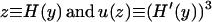
The proof of part iii is trivial and we omit it. For the remaining part of the proof we may assume without loss of generality that V = 1 and κ = ɛ = 1; indeed, if H(y) is a solution to problem 3.4 with V = 1 and κ = ɛ = 1, then the function

is a solution to problem 3.4 at any positive κ, ɛ, and V.

So let V = 1 and κ = ɛ = 1. Integrating the equation once, we end up with the problem

3.9

We claim that any solution H(y) to problem 3.9 satisfies

3.10

Because H‴ > 0 near y = 0 there exists

and hence there exists

If the latter limit is finite, then H‴(y) ≥ Cy⁻³ near y = 0 for some positive constant C, and three integrations yield a contradiction with the boundedness of H as y → 0⁺: hence H′(y) → +∞ as y → 0⁺ and we have proved the asymptotic relation 3.10.

According to 3.10 we may assume that y₀ is so small that H′(y) > 0 if 0 < y < y₀, which allows us to use H as an independent variable: setting

and using the relations dz/dy = H′ = u^1/3, H" = u^−1/3u′ and H‴ = u" − (u′)²/u, we obtain the new problem

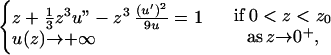3.11

where z₀ = H(y₀). Now we prove the following statements

(i)  Let z₀ in 3.11 be positive and let u(z) be a smooth and positive solution of problem 3.11. Then there exist A, B ∈ R such that as z → +∞,

3.12

where

(ii)  For any A, B ∈ R there exists z₀ > 0 such that the problem 3.11 has a unique smooth and positive solution u(z) satisfying 3.12.

First we observe that u = 9/5z is a solution to the equation z³u" − z³(u′)²/9u = 1. We introduce new variables

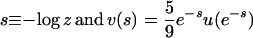and obtain the equation for v

3.13

Any positive solution of 3.13 satisfies the limiting relations

3.14

Indeed, accepting 3.14 for the moment, we observe that the general solution to the equation

is given by

3.15

where μ = /6, and it follows from 3.15 and standard linearization techniques that the solutions of 3.13 and 3.14 form a two-parameter family described by

Transforming this expression back in terms of u and z and redefining A and B, we finish the proof of our statement 3.12.

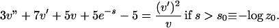
It remains now to prove 3.14. The function

satisfies the equation

if s > s₀. Multiplying the equation by w′ and setting

we obtain

and since F(p) is a strictly convex function which attains its minimum at p = 1, 3.14 follows at once.

The relation 3.12 implies that, as y → 0⁺,

or equivalently,

3.16

Because

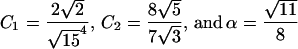
for certain constants à and B̃, integrating 3.16, redefining A and B, and setting C₁ = (64/15)^1/4, we obtain that, as y → 0⁺,

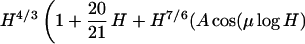Hence as y → 0⁺,

or, redefining A and B again, we obtain

This completes the proof of the basic relation 3.7.

Section 4. A Class of the Self-Similar Solutions

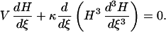
The equation 1.1 possesses a set of self-similar solutions under some special assumptions concerning the functions h₀(dx₀/dt), G(dx₀/dt), and C(dx₀/dt) which enter the boundary conditions 1.2 at the contact lines x = ±x₀(t). Depending on the values of parameters, these solutions belong to the first or the second kind.

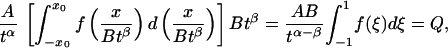
Indeed, assume that the functions h₀(dx₀/dt), G(dx₀/dt), and C(dx₀/dt) are power monomials. In this case the boundary conditions 1.2 at x = x₀(t) (we consider a symmetric case) take the form

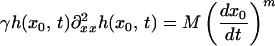4.1

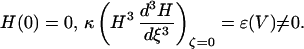
Here K, M, N, k, m, n are constants; the remaining notations are the same as previously. Due to the symmetry of the film spreading, the solution can be considered in the interval 0 ≤ x < ∞, and the boundary condition at x = 0 should be added:

4.2

Under the assumed special conditions the self-similar solution takes the form

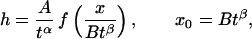4.3

where A, B, α, β are positive constants, and α and β are dimensionless. When we substitute 4.3 into Eq. 1.1 we obtain the following relation between the constants α and β:

4.4

which is necessary to avoid the explicit appearance of time in the coefficients of the resulting ordinary differential equation for the function f(ζ), where ζ = x/Bt^β:

4.5

Furthermore, substituting 4.3 into the first boundary condition 4.1, we obtain a relation:

from which two further relations follow:

4.6

and

4.7

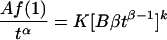
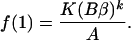
The function f(ζ) can be renormalized; therefore there exists a relation between the constants A and B. We may choose it in such a way that f(1) = 1, so that

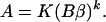4.8

In a way similar to 4.6, 4.7 the relations for m and n can be obtained from the second and third conditions 4.1

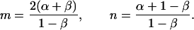4.9

Taking into account the first condition in the form

4.10

we obtain the second and the third conditions at ζ = 1 for the function f(ζ):

4.11

and

4.12

From 4.2 it also follows that

4.13

We assume for simplicity that M = 0 (negligible tangential force at the tip region), then the condition 4.11 is reduced to

4.14

The constant B and the second relation between α and β remain so far undetermined. Here the situation is different in principle in the cases N = 0 and N ≠ 0, i.e., in the cases where there is no inflow or outflow through the tip region, and where such outflow/inflow exists.

In the case N = 0 an integral conservation law holds:

4.15

where the constant parameter Q is known from the initial conditions.

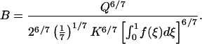
The relations 4.3 and 4.8 give

from which the basic relations follow:

4.16

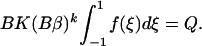4.17

From 4.4 and 4.16 we obtain

4.18

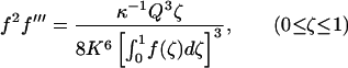
so that according to 4.6, k = . Under condition 4.18 the first integral of equation 4.5 can be obtained. Using conditions 4.13 and 4.18, the following relationship appears

4.19

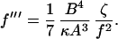
Furthermore, from 4.17 we obtain

4.20

This relation can be rewritten as

4.21

It is interesting to note a singularity in 4.21 which appears at K = 0, i.e., at h₀ = 0 (cf. the previous section).

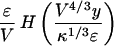
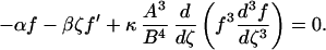
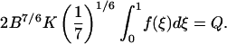
The construction of the self-similar solution reduces to the study of the nonlocal boundary value problem

4.22

In a forthcoming paper we shall prove the existence of a solution for any value of Q/κ^1/3K². In addition, we study its qualitative properties for large values of Q/κ^1/3K², which is expected to be the physically interesting case. If Q/κ^1/3K² ≫ 1, then f(0) ≫ 1 and the shape of the corresponding self-similar solution h(x, t) at fixed t is a parabola in the major part of the film; this result indicates the existence of two different time scales: away from the contour region the equilibrium is reached on a relatively short time scale.

In the same way the solution for the axisymmetric case can be constructed, in this case α = , β = . An attempt to construct this solution was performed by Starov (31) (see also ref. 32), but he did not use the proper boundary conditions.

In the case N ≠ 0 the integral conservation law does not exist, the second relation between the constants α and β should be obtained by solving a nonlinear eigenvalue problem, and the constant B remains undetermined. This is a typical situation for self-similar solutions of the second kind.

Section 5. Conclusion

The basic system 1.2 and the simplified system of free boundary conditions 2.13–2.15 obtained in this paper are essentially different from the systems discussed previously in the literature. First of all, the contact angle as a function of velocity should not be prescribed. According to 2.14 the contact line consists of the inflection points of the film surface, and condition 2.15 gives the nonzero flux at the contact line without introducing new functions other than h₀(dx₀/dt). In principle the system of boundary conditions 1.2 is of the same type as 2.13–2.15 but requires more information concerning the prescribed functions of the velocity. An instructive special case of the system 2.13–2.15 leads to a self-similar solution of the first kind, which is also considered in this paper.

References

- 1.Greenspan H P. J Fluid Mech. 1978;84:125–143. [Google Scholar]
- 2.Huh, C. & Scriven, L. E. (1971) J. Colloid Interface Sci., 85.
- 3.Dussan V, E B, Davis S H. J Fluid Mech. 1974;65:71–95. [Google Scholar]
- 4.Dussan V, E B. Annu Rev Fluid Mech. 1979;11:371–400. [Google Scholar]
- 5.Ngan C G, Dussan V, E B. J Fluid Mech. 1989;209:191–226. [Google Scholar]
- 6.Dussan V, E B, Ramé E, Garoff S. J Fluid Mech. 1991;230:97–116. [Google Scholar]
- 7.Hocking, L. M. (1981) Q. J. Mech. Appl. Math. 34, Part 1, 37–55.
- 8.Calliadasis S, Chang H-C. Phys Fluids. 1994;6:12–23. [Google Scholar]
- 9.Lacey A A. Stud Appl Math. 1982;67:217–230. [Google Scholar]
- 10.De Gennes, P. G. (1985) Rev. Mod. Phy. 57, Part 1, 827–863.
- 11.Bertozzi A L, Brenner M P, Dupont T F, Kadanoff L P. Ryerson Lab Report. Chicago: Univ. Chicago; 1993. [Google Scholar]
- 12.Oron A, Davis S H, Bankoff S G. Applied Mathematics Technical Report No. 9509. IL: Northwestern Univ. Evanston; 1996. [Google Scholar]
- 13.Shikhmurzaev Yu D. J Fluid Mech. 1997;334:211–250. [Google Scholar]
- 14.Bernis F, Friedman A. J Diff Eq. 1990;83:179–206. [Google Scholar]
- 15.Bernis, F. (1995) in Free Boundary Problems 1993, Toledo, Spain, Pitman Research Notes in Mathematics, eds. Diaz, J. I., Herrero, M. A., Liñan, A. & Vázquez, J. L., pp. 40–56.
- 16.Bertozzi, A. L. (1995) in Free Boundary Problems 1993, Toledo, Spain, Pitman Research Notes in Mathematics, eds. Diaz, J. I., Herrero, M. A., Liñan, A. & Vázquez, J. L., pp. 72–85.
- 17.Bernis F, Peletier L A, Williams S M. Nonlin Anal. 1992;18:217–234. [Google Scholar]
- 18.Beretta E, Bertsch M, Dal Passo R. Arch Rat Mech Anal. 1995;129:175–200. [Google Scholar]
- 19.Bertozzi A L, Pugh M. Commun Pure Appl Math. 1996;49:85–123. [Google Scholar]
- 20.Boatto S, Kadanoff L P, Olla P. Phys Rev E. 1993;48:4423. doi: 10.1103/physreve.48.4423. [DOI] [PubMed] [Google Scholar]
- 21.Bernis F. Adv Diff Eq. 1996;1:337–368. [Google Scholar]
- 22.Bernis F. C R Acad Sci Paris, Sér I. 1996;322:1169–1174. [Google Scholar]
- 23.Dal Passo R, Garcke H, Grün G. SFB 256. 1996. p. preprint. no. 467. [Google Scholar]
- 24.Bertsch, M., Dal Passo, R., Garcke, H. & Grün, G. (1997) Adv. Diff. Eq., in press.
- 25.Batchelor G K. An Introduction to Fluid Dynamics. Cambridge, U.K.: Cambridge Univ. Press; 1967. [Google Scholar]
- 26.Dzyaloshinskii I E, Lifshitz E M, Pitaevski L P. Sov Phys JETP. 1960;10:161–170. [Google Scholar]
- 27.Barenblatt G I. Adv Appl Mech. 1962;7:55–129. [Google Scholar]
- 28.Barenblatt, G. I. (1995) in Free Boundary Problems 1993, Toledo, Spain, Pitman Research Notes in Mathematics, eds. Diaz, J. I., Herrero, M. A., Liñan, A. & Vázquez, J. L., pp. 20–39.
- 29.Van Dyke M D. Perturbation Methods in Fluid Mechanics. 2nd Ed. Stanford, CA: Parabolic; 1975. [Google Scholar]
- 30.Cole J D. Perturbation Methods in Applied Mathematics. Toronto: Blaisdell; 1968. [Google Scholar]
- 31.Starov V M. J Colloid Interface Sci USSR. 1983;45:1154. [Google Scholar]
- 32.Brenner M, Bertozzi A. Phys Rev Lett. 1993;71:593–596. doi: 10.1103/PhysRevLett.71.593. [DOI] [PubMed] [Google Scholar]