Analysis of linear trade models and relation to scale economies

Abstract

We discuss linear Ricardo models with a range of parameters. We show that the exact boundary of the region of equilibria of these models is obtained by solving a simple integer programming problem. We show that there is also an exact correspondence between many of the equilibria resulting from families of linear models and the multiple equilibria of economies of scale models.

In Gomory and Baumol (1), we discussed the equilibria that arise from the classical linear Ricardian model of international trade when the productivity parameters e_i,j of the model are allowed to vary, limited only by a maximal productivity constraint, e_i,j ≤ e_i,j^max. We plotted each equilibrium as a point in a (Z₁, U₁) diagram, where Z₁ is country 1’s share of total world income, Z₁ = Y₁/(Y₁ + Y₂), and U₁ is the utility of country 1 at that equilibrium. We had similar diagrams in which we plotted (Z₂, U₂), where Z₂ = 1 − Z₁ is country 2’s share and U₂ is country 2’s utility.

We showed that in each case the resulting region of equilibria (R₁ for country 1 and R₂ for country 2) could be bounded above by a curve B_j(Z₁) obtained by solving a very simple linear programming problem for each value of Z₁. This upper bounding curve has a characteristic hill shape that persists over a wide range of models. Furthermore, as the number of industries in the model increases, we showed that the actual upper boundary of the region rapidly approaches this boundary curve.

The economic significance of these results comes from the characteristic hill shape of the region of equilibria. The hill shape implies that there is inherent conflict in international trade, that the best equilibria for one country are poor ones for the other, and that a country is better off with a partly developed trading partner than with a fully developed one. The fundamental mechanism at work is complementary to but different from the mechanisms employed in the analyses of international trade that also have shown the possibility of conflict in Hicks (2), Dornbush et al. (3), and Krugman (4). An excellent summary of the relevant history appears in Grossman and Helpman (5).

In this note we complete one component of this analysis by showing that the upper boundary of the region is given exactly by solving a closely related integer programming problem. The relation between the linear programming problem and the integer programming problem is that they are two different relaxations of the economies of scale problem introduced in Gomory (6). We discuss the close connection between the linear family and economies of scale models below.

This result enables us to examine models with a small number of products; models in which there is a considerable gap between the boundary given by the linear programming approximation and the actual boundary of the region of equilibria. This includes, for example, the famous model of trade in textiles and wine given by David Ricardo. These small models can and do turn out to have special characteristics, due to their small size, that disappear in all but the most contrived large models. These characteristics cause small models not to exhibit the inherent conflict that is present in almost all large models.

The Exact Boundary Theorem

As in Gomory (6) and Gomory and Baumol (7), we use x_i,j for the market share of country j in the ith industry. We again use Z_C for the classical income-share value, which here is simply the income share of the countries when e_i,j = e_i,j^max. We use the same linearized utility

1

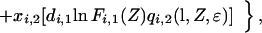
which is the same as the Cobb–Douglas utility at every equilibrium, to measure utility. In Eq. 1, ɛ is the vector {e_i,j} of productivities per unit of (labor) input and F_i,j(Z) is country j’s consumption share of the ith good derived from a Cobb–Douglas utility, so F_i,j(Z) = d_i,jZ₁/(d_i,2Z₁ + d_i,2Z₂). q_i,j in Eq. 1 is the quantity of good i produced in country j when it is the sole producer of i, so that

2

In Eq. 2, w_j is the wage level in country j and L_j is country j’s labor-force size. With this notation we assert the following theorem:

Exact Boundary Theorem. The upper boundary B_I,1(Z) of the region of equilibria R₁ for Z₁ ≤ Z_C is the solution of the maximization problem in integer x:

3a

while for Z₁ ≥ Z_C it is the solution of

3b

Note that the ɛ that appears in the linearized utility in the theorem is ɛ^max = {e_i,j^max}, the vector of maximal productivities.

Proof: Part 1. B_I,1(Z₁) lies above any equilibrium. Consider any equilibrium (x, Z₁, ɛ) with market shares x, productivities ɛ, and income share Z₁ ≤ Z_C, so that Eq. 3a applies. The market shares x satisfy the inequality in Eq. 3a as an equality. From x construct an integer x′ by setting x′_i,1 = 1 and x′_i,2 = 0 in the industries where country 1 is the sole producer and x′_i,1 = 0, x′_i,2 = 1 in all other industries. This new integer x′ has less producing industries in country 1 (x′_i,1 ≤ x_i,1). So x′ satisfies the inequality in Eq. 3a and is, therefore, a feasible integer solution to Eq. 3a. The objective function value for x′, Lu(x′, Z₁, ɛ^max), is also greater than or equal to the utility Lu(x, Z₁, ɛ) of the original equilibrium. This can be seen by a term-by-term (industry-by-industry) comparison of Lu(x′, Z₁, ɛ^max) with Lu(x, Z₁, ɛ). If the ith industry had only one producer in x, for example x_i,1 = 1, it still has only one producer in x′, so the only change is the replacement of e_i,1 by e_i,j^max, which only increases utility. If, however, the ith industry was shared in x, it now has x′_i,2 = 1 in x′. But for shared industries both countries produce at the same cost so e_i,1/w₁ = e_i,2/w₂ and we can see from Eq. 2 that q_i,1 = q_i,2. Therefore, the shift in x does not by itself affect the linearized utility. We then argue, as we just have done for the specialized industries, that the coefficient of x′_i,2 is greater than the coefficient of x_i,2 and this only increases utility. So Lu(x′, Z₁, ɛ^max) ≥ Lu(x, Z₁, ɛ). Because for any equilibrium (x, Z₁, ɛ) we can construct the corresponding integer x′, B_I,1(Z₁), the maximum over integer solutions must be as large as the utility of any equilibrium with share Z₁.

Proof: Part 2. There is an equilibrium with the same linearized utility as B(Z). Let x be the maximizing solution to the integer programming problem for that same Z₁. Since Z₁ < Z_C, we know from Gomory (6) or Gomory and Baumol (1) that with market shares x satisfying the inequality in Eq. 3a, there is an industry in which country 1 can be the cheaper producer, but in which it is not producing. In symbols, there is an i for which e_i,1^max/w₁ > e_i,2^max/w₂, but x_i,1 = 0. If we increase this x_i,1, the objective function increases. If we increase x_i,1 to 1, we have a new integer x with a larger value of the objective function. Since x was already the maximizing integer solution satisfying Eq. 3a, we must conclude that increasing x_i,1 to 1 must have violated the inequality in Eq. 3a. Therefore, there is a value of x_i,1 < 1 that produces equality in Eq. 3a. We adopt this value of x_i,1 thus forming a new vector x′ with one noninteger component. We next choose a new smaller value for e_i,1 that makes both countries equally cheap producers in industry i; that is, we choose e_i,1 so that e_i,1/w₁ = e_i,2^max/w₂. With this new e_i,1, no change in utility results in going from x to x′. But x′ now has share Z₁ and satisfies the conditions for an equilibrium. Thus we have produced an equilibrium with share Z₁ and with a linearized utility value as great as the maximizing integer solution. Parts 1 and 2 together prove the theorem for equilibria with Z₁ ≤ Z_C; the proof for Z₁ ≥ Z_C is almost identical.

Using the Exact Boundary Theorem

We can solve Eqs. 3a and 3b by using standard integer programming techniques. Our model is in fact the simplest of all integer programming problems, the knapsack problem. We have solved a series of small problems by using dynamic programming to obtain the data in the figures below. Although our techniques allow us to catalogue all small models, we will not do that, but rather we will watch the evolution of one small model as the number of industries increases.

Fig. 1 shows the results for Ricardo’s classical textile-wine example. There are only two industries. Country 1 (England) excels in one of them (textiles), so that e_1,1^max = 1 whereas e_1,2^max = 0.55, and the other country (Portugal) excels in the other industry (wine), so that e_2,2^max = 1 and e_2,1^max = 0.45. All equilibria with e_i,j ≤ e_i,j^max are plotted. In Fig. 1A we have plotted world output as measured by country 1’s utility function. In Fig. 1B we show country 1’s utility, and in Fig. 1C we show country 2’s utility measured in country 2 utility units. The boundary in Fig. 1B is simply the boundary in Fig. 1A multiplied by country 1’s share of world income, Z₁. The boundary in Fig. 1C would be world output utility multiplied by country 2’s share if the world output were measured by country 2’s utility. There is a sharp peak in world output above the classical level Z_C. This is where England specializes in textiles and Portugal specializes in wine, and both have attained maximal productivity. This peak is high enough that the best outcome for each country is attained there, as Fig. 1 B and C shows. So in the two-product case, the classical specialized outcome is the best possible result for both countries. But this is far from typical.

Figure 1.

(A) Two industries, world utility. (B) Two industries, country 1 utility. (C) Two industries, country 2 utility.

In the three-industry model shown in Fig. 2, country 1 is better in two industries with combined demand somewhat less than the demand for the one industry in which country 2 is best. We show world utility in Fig. 2A, together with country 1’s utility, and the utility of country 2 in Fig. 2B. Although the classical level is still good for both countries, there are points to the left in Fig. 2B that are about as good for country 2.

Figure 2.

(A) Three industries, world and country 1 utility. (B) Three industries, country 2 utility.

In Fig. 3, a four-industry model, country 1 is better in two industries and country 2 is better in two industries. We have combined all the utilities in a single figure. Country 1 utility is read from the right vertical axis and country 2 utility is read from the left. Already the best equilibrium is clearly different for the two countries.

Figure 3.

Four industries, all utilities.

In Fig. 4, a six-industry model, we have added the smooth linear (not integer) programming boundaries that we referred to in the introduction. Note that they are already close to the exact boundaries and that the equilibria best for the two countries are clearly different from one another. As in Gomory and Baumol (1), the equilibrium that is best for country 1 is rather poor for country 2 and vice versa. We have returned to the inherent conflict that in Gomory (6) characterizes models with large n. This is avoided only in the models with the very smallest number of products.

Figure 4.

Six industries, all utilities and linear programming boundaries.

The Connection with Scale Economies Models

All of this, together with our earlier work, point to a close connection between families of linear models and models with economies of scale. We have explored that connection in Gomory and Baumol (7) and summarize it herein as follows:

The Correspondence Principle.

We say that a scale-economies model M(f_i,j) corresponds to a linear family model if it has the same labor-force sizes L₁ and L₂ and the same country demand values d_i,j. However, instead of linear production functions e_i,jl_i,j, the model M(f_i,j) has production functions f_i,j(l) with economies of scale, defined as nondecreasing average productivity, f_i,j(l)/l. We assume that there is a well-defined derivative df_i,j(l)/dl at l = 0 and that f_i,j(L_j)/L_j, which is the largest productivity value that f_i,j(l)/l can attain in the model, is e_i,j^max.

Theorem 5.1 (Correspondence Theorem). From any specialized equilibrium (x, Z₁) of the scale-economies model, we can construct a corresponding equilibrium (x, Z₁, ɛ) of the linear family having the same x and Z₁ and an ɛ given by: (i) the e_i,j for producers is average productivity at the economies equilibrium, so e_i,j = f_i,j (l_i,j)/l_i,j, and (ii) the e_i,j for nonproducers is marginal productivity at output zero, so that e_i,j = df_i,j(0)/dl_i,j.

Many Corresponding Equilibria.

If the economies model has many equilibria, each will clearly correspond to a different equilibrium (x, Z₁, ɛ) of the family of linear models. One economies model is, therefore, a way of looking at a large sample of the equilibria of a family of linear models. Fig. 5 shows the (linear programming) boundary for country 1’s region of equilibria from a linear family model, together with the equilibrium points corresponding to one rather small economies model. The set of economies equilibria display the characteristic shape described in Gomory (6).

Figure 5.

Country 1 utility and economies equilibria.

The location of the equilibria corresponding to M(f_i,j) in the region of equilibria of the linear family depends on the nature of the scale economies. If the production functions f_i,j(l) have productivities f_i,j(l)/l that go on increasing until l = L_j, the corresponding equilibria tend to be low in the region of equilibria of the linear models. This is because equilibrium labor quantities l_i,j are generally small compared with the size of the entire work force L_j. Therefore, the e_i,j = f_i,j(l_i,j)/l_i,j that they produce in the corresponding equilibria will tend to be small compared with e_i,j^max = f_i,j(L_i,j)/L_i,j. This results in equilibria with relatively low productivity and low utility levels. On the other hand, if the production functions have already reached full economies of scale when each country is supplying its own needs in autarky, the corresponding equilibria are high up in the region. In fact they are all maximal productivity equilibria, because e_i,j = f_i,j(l_i,j)/l_i,j = f_i,j(L_i,j)/L_i,j = e_i,j^max. Fig. 5 shows a model with mild scale economies, so that the dots representing equilibria from the economies model are part way up the country 1 region.

Theorem 5.3 (Maximal Productivity Correspondence Theorem). The 2ⁿ − 2 specialized maximal productivity equilibria always correspond to the equilibria of a single economies model.

References

- 1.Gomory R E, Baumol W J. Proc Natl Acad Sci USA. 1995;92:1205–1207. doi: 10.1073/pnas.92.4.1205. [DOI] [PMC free article] [PubMed] [Google Scholar]
- 2.Hicks J R. Oxford Economic Papers. 1953;5:117–135. [Google Scholar]
- 3.Dornbush R, Fischer S, Samuelson P A. American Economic Review. 1977;67:823–839. [Google Scholar]
- 4.Krugman P R. In: Structural Adjustment in Developed Open Economies. Jungenfelt K, Hague D, editors. London: Macmillan; 1986. pp. 35–49. [Google Scholar]
- 5.Grossman G M, Helpman E. Technology and Trade. Cambridge, MA: National Bureau of Economic Research; 1994. , Working Paper 4926, pp. 1–73. [Google Scholar]
- 6.Gomory R E. J Econ Theory. 1994;62:394–419. [Google Scholar]
- 7.Gomory R E, Baumol W J. Linear Trade-Model Equilibrium Regions, Productivity, and Conflicting National Interests, C. V. Starr Economic Research Report 9631. New York: New York Univ.; 1996. [Google Scholar]