Control of time-dependent biological processes by temporally patterned input

Abstract

Temporal patterning of biological variables, in the form of oscillations and rhythms on many time scales, is ubiquitous. Altering the temporal pattern of an input variable greatly affects the output of many biological processes. We develop here a conceptual framework for a quantitative understanding of such pattern dependence, focusing particularly on nonlinear, saturable, time-dependent processes that abound in biophysics, biochemistry, and physiology. We show theoretically that pattern dependence is governed by the nonlinearity of the input–output transformation as well as its time constant. As a result, only patterns on certain time scales permit the expression of pattern dependence, and processes with different time constants can respond preferentially to different patterns. This has implications for temporal coding and decoding, and allows differential control of processes through pattern. We show how pattern dependence can be quantitatively predicted using only information from steady, unpatterned input. To apply our ideas, we analyze, in an experimental example, how muscle contraction depends on the pattern of motorneuron firing.

When measuring input–output relations in biological systems, it is often observed that the magnitude of the output depends not just on the magnitude of the input, but also on its temporal pattern—its arrangement in time. The pattern of firing of a neuron—to cite the most notable example—is found to modulate seemingly every activity-dependent variable, including the spread of the electrical activity within the neuron (1), transmitter and hormone release (2–8), postsynaptic integration of the signal (9), levels of second messengers (8, 10, 11), as well as more complex consequences such as synaptic plasticity (12–14), regulation of ion-channel complements (15–17), neurite growth and motility (11, 18), and gene expression (11, 19, 20). Another output variable that is modulated by neuronal firing pattern is muscle contraction (21–25). Fig. 1 shows a dramatic example of this in a well known preparation, the accessory radula closer (ARC) neuromuscular system of Aplysia (26–29). Even though all five motorneuron firing patterns shown contain the same mean density of spikes, they produce very different peak, and more importantly mean, levels of contraction. Further examples of pattern dependence are found in biochemical systems, for instance in response to different frequencies of oscillation in levels of hormones and intracellular second messengers (30, 31).

Figure 1.

Pattern and pattern dependence: definitions and examples. (A) Specification of the input waveforms used throughout this work. t, time; i, input amplitude; 〈i〉, mean i; P, period; F, duty cycle; ℐ₀, unpatterned waveform of steady input at i = 〈i〉; ℐ_x, a patterned waveform of three times higher input for one-third of the time. (B) Dependence of contraction of the ARC muscle of Aplysia on (C) the pattern of motorneuron firing. Experiments were done as in (28, 29). Motorneuron B15 [(26); B15 was used in all experiments presented in this paper; results with B16 were similar] was intracellularly stimulated to fire spikes [individual spikes were driven by separate brief current injections (28), not shown] in the desired pattern, always of the form in A. The firing frequency was taken as the input variable i and contraction amplitude as the output variable o (A13). Contractions were isotonic and unloaded; length was monitored with an isotonic transducer. ō, peak contraction; 〈o〉, mean contraction. With steady, unpatterned firing (waveform ℐ₀), the contraction reaches the steady state ō(ℐ₀) = 〈o〉(ℐ₀) (Left); with patterned firing (waveforms ℐ_x), it reaches different values ō(ℐ_x) and 〈o〉(ℐ_x), as indicated for the rightmost pattern. By Eq. 2, normalizing the values for ℐ_x by that for ℐ₀ establishes the scale of absolute pattern dependence Φ, shown on the right of B.

Temporal pattern dependence is thus a very common phenomenon; indeed, it will be one of our conclusions here that it is necessarily ubiquitous. However, beyond the basic observations of its presence, its study has been limited by the lack of a conceptual framework with which to quantitatively define, understand, and predict pattern dependence in biological systems. In this paper, we shall develop such a framework. We shall then use the experimentally advantageous ARC-muscle system to illustrate and test our ideas.

Formalization of the Problem

To be able to see under what circumstances pattern dependence can, or cannot, arise, we must first pose the question, and define “pattern” and “pattern dependence,” more precisely. (Nevertheless, from the mathematical standpoint, our presentation and notation in this paper is informal, aiming at an intuitive sketch of the main points rather than complete precision. More technical matters are noted in Appendices A1–A14.)

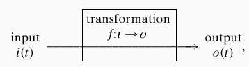
Consider an arbitrary input–output relation

1

where i, and therefore o, varies with time, t. Our question becomes: what forms of f are sufficient or necessary for patterns in i to affect such properties of o as its peak (ō) and mean (〈o〉) amplitude?

Clearly, pattern is a property of an interval of time; we can suppose i to be periodic and study one period, P. For simplicity, we shall in this paper concern ourselves only with steady-state pattern dependence, after i has been applied sufficiently long for o to be invariant in successive periods. Let I = ∫_P i dt, the “amount” of i in P, and 〈i〉 = I/P, the mean i. Similarly, 〈o〉 = (1/P)∫_P o dt. Any particular input waveform ℐ_x [i.e., the sequence i_x(t), t∈P] is completely defined by 〈i_x〉 and the distribution of I_x over P—the pattern. Both properties will affect o. Given only one input waveform or waveforms differing in both properties, with f unknown, the effect of pattern is indeterminate (see AppendixA1). [This has obvious experimental implications (A2).]

To isolate the effect of pattern, we therefore consider further only waveforms with the same 〈i〉, which differ only in pattern. In particular, we shall use sets of waveforms of the sort shown in Fig. 1 A and C, where each waveform ℐ_x concentrates the same I > 0 into a single block of i_x = 〈i〉/F_x occupying a different fraction 0 < F_x ≤ 1 of P (i.e., F is the “duty cycle”). Such waveforms are a natural representation of a variety of biological patterns—in Fig. 1, the grouping of neuronal spikes into bursts—and can serve as elementary constituents of more complex waveforms. (Square waveforms of this sort are also used in most experimental work.) Our qualitative conclusions will be applicable to patterns more generally (even irregular patterns: see A14), but this subset will serve as a test case for which we shall perform the analysis of pattern dependence in quantitative terms (A3).

It is convenient to always include in our set of waveforms the special waveform ℐ₀ with F₀ = 1, i₀ = 〈i〉—steady input with no pattern. In this case, we can write the ratios of the output with patterned input to that with steady, unpatterned input,

2

for the absolute dependence Φ of the peak (ō) and mean (〈o〉) output on the pattern x imposed on mean input 〈i〉. Generally, of course, ō(ℐ₀) = 〈o〉(ℐ₀) (A4), and, since 〈o〉(ℐ_x) ≤ ō(ℐ_x), Φ_〈o〉 ≤ Φ_ō. All of this is indicated graphically in Fig. 1.

We find that the mean output is pattern independent (Φ_〈o〉 = 1) if and only if f is a linear transformation (A5 and A6). If f(i) = constant, Φ_ō = 1 also. In any case, as long as f is instantaneous, the value of P is immaterial.

Properties of Biologically Important Transformations.

To actually compute Φ, we must specify f. We shall now specify f that is itself time dependent (A4), implicit in the differential equation describing the kinetic schema

3

(where 0 ≤ a ≤ 1; α, β, p, q, constants; q = 1, 2, 3 …) (A7). Rather than producing o directly, i now controls the rate of a reaction that produces o. This is a natural way to think of many biological mechanisms, and schema 3 is representative of schemata used throughout biophysics, biochemistry, and physiology (32–38). Such schemata share three important properties that are a universal feature of real biological processes: nonlinearity, saturability, and time dependence that can be described by a characteristic time constant (A8). Since it will be these properties that determine our qualitative conclusions, these again will be applicable well beyond the exact form of schema 3, which is just one particular form specified for the purposes of quantitative analysis.

Properties of Pattern Dependence

Given any f and any input waveform, we can compute Φ. This can always be done numerically. However, for our canonical waveforms as input to the simple f given by schema 3, we can obtain analytical solutions, because we can explicitly integrate the differential equation involved (A9). This yields the time course of a, and thus of o, as they rise and fall during the two phases of the pattern (see Fig. 2F). The requirement that in the dynamical steady state of the system the rise and fall must be equal fixes the absolute elevation of the output waveform, and so gives ō and 〈o〉. Thus, in the dynamical steady state reached with patterned i, just as in the true steady state reached with steady i, we are able to convert knowledge of the kinetics of o into knowledge of its absolute amplitude.

Figure 2.

Theoretical properties of pattern dependence, with transformation f given by schema 3. (A–C) For three representative cases, Φ_ō (Left) and Φ_〈o〉 (Right) are plotted as functions of the pattern (F, P), using Eqs. 6 and 7 in A9. Coordinates as well as locations of the line P ≈ τ (A8) and surface Φ = 1 are indicated in the upper middle diagram. Φ = 1 is represented in medium gray, Φ > 1 lighter, and Φ < 1 darker. In all cases α,β = 1, p and q are as indicated, and 〈i〉 = 0.01 (A) or 0.25 (B and C). These values of 〈i〉 were chosen to give o_∞(〈i〉) ≈ 0.01 and τ ≈ 1 in all three cases. (D) Linear plot of the circled region in C. (E) The steady-state f: o_∞ − i relations for the three cases in A–C (A10). For P ≫ τ, Φ_ō and Φ_〈o〉 may be computed from such relations as follows. As F3 shows, ō(ℐ_x) = o_∞(i_x) and 〈o〉(ℐ_x) = Fo_∞(i_x), and of course ō(ℐ₀) = 〈o〉(ℐ₀) = o_∞(〈i〉). Then, from Eq. 2, Φ_ō = o_∞(i_x)/o_∞(〈i〉) and Φ_〈o〉 = Fo_∞(i_x)/o_∞(〈i〉 = Fφ_ō). Setting Φ_ō = 1 and Φ_〈o〉 = 1 yields equations for the two lines shown. For any particular 〈i〉 and F [here illustrated for 〈i〉 on curve B and F = 0.5, so that i_x = 2〈i〉], defining the points 1–4 as shown and writing o_∞,1 for the o_∞ value at point 1, etc., we see that Φ_ō = o_∞,2/o_∞,1 = o_∞,2/o_∞,4 and φ_〈o〉 = Fo_∞,2/o_∞,1 = o_∞,2/o_∞,3. (Φ is much smaller here than in A–C because 〈i〉 is much larger.) Φ can thus be computed even from a purely empirical o_∞−i relation. In this theoretical case, of course, we know the precise equivalent general expressions for Φ (A10). (F) Time courses of o at the three locations indicated in A—i.e., the solutions (A9) of schema 3 (Eq. 5) with α, β, p, q = 1 (since q = 1, these are also the time courses of a), for the input waveforms ℐ₀ and ℐ_x with 〈i〉 = 0.01, F = 1/3, i_x = 3〈i〉 (Bottom), when P ≪ τ (F1), P ≈ τ (F2), and P ≫ τ (F3).

Thus, we can derive analytical expressions giving Φ_ō and Φ_〈o〉 for any pattern x in terms of α, β, p, q, and 〈i〉 (A9). Because f is time dependent, we must now include P in the specification of x. With our waveforms, any pattern x is uniquely defined by the pair (F, P), allowing x to be plotted in two dimensions and Φ in the third (A3). This is what we have done in Figs. 2 A–C and 3C; Figs. 3E and 4 show sections at a single F. (In Figs. 2 A–C and 4, extended log scales are used to emphasize the asymptotic behavior at extremes, but, as the linear plot in Fig. 2D shows, only fairly small, physiological changes in F and P are in fact needed to change Φ substantially.)

Figure 3.

Experimental analysis of pattern dependence in the Aplysia ARC-muscle system. (A and B) Contraction kinetics and o_∞−i relations (from the experiment in B and two others) obtained with steady, unpatterned motorneuron firing (schematically indicated under B). To summarize the data for the purposes of computation, we fitted the kinetics, at each i, with a delay d(i), then a single-exponential rise with time constant τ(i), to the steady-state amplitude o_∞(i) (thin, smooth curves in B). Though the actual kinetics are clearly more complex, this form appeared to provide the most simple yet reasonably adequate empirical description of the data. (C) Φ_ō and Φ_〈o〉 predicted from the values obtained from A and B (mesh; computed using the same strategy as in A9) and experimentally measured (scatter points; steady-state measurements as in Fig. 1 B and C). The measured values are from 11 preparations, which gave surfaces of Φ of similar shape but different absolute amplitude. The values from each preparation were therefore scaled so as to normalize the reference value Φ(F = 0.5, P = 10 s) to the mean from all preparations (Φ_ō, 27 ± 19 SD, range 13–75; Φ_〈o〉, 14 ± 9 SD, range 6–37). The mean 〈i〉 was 5.7 Hz (±1.2 SD, range 4–8); the same value was used in the theoretical computations. The mean deviation of the experimental points from the predicted surface is 3.4 for Φ_ō, 1.0 for Φ_〈o〉 (n = 132, values for F = 1 excluded). (D) Cooling the preparation (here from 20.3 to 14.9°C; unpatterned firing at 4 Hz) greatly increases contraction amplitude. (E) Concomitantly, cooling greatly reduces Φ. Means ± SEM from four preparations (not normalized) first at 20–21.1°C, then 14.9–15°C. 〈i〉 = 4–5.5 Hz; F = 0.25. [The experiments in Figs. 1 B and C and 3 A–C were done at the “warm” temperatures. All temperatures used are in the physiological range for Aplysia (40).]

Figure 4.

Different processes can be tuned to respond to different patterns of the same input variable. This is, essentially, a section through the φ_〈o〉 surface in Fig. 2C (thus p = 1, q = 3, 〈i〉 = 0.25) at F = −3 for three processes with time constants two orders of magnitude apart: process 1, α = 400, β = 1,000; process 2, α = 4, β = 10; process 3, α = 0.04, β = 0.1. “Windows” of pattern dependence such as these are observed experimentally (11, 19, 20).

As f is nonlinear, we expect pattern dependence. However—and this is the key point—the nonlinearity only appears on time scales longer than τ, the time constant of f (A8). The input pattern exists on time scales shorter than P. Only when P > τ, so that the nonlinearity and the pattern overlap and interact, does the pattern dependence become expressed (A6).

This can be seen in Fig. 2 A–C, which are plots of the surfaces of Φ_ō and Φ_〈o〉 for three representative cases. In the P direction, each plot is divisible into two regions of distinct Φ, above and below P ≈ τ. [In the F direction, Φ(F = 1) = 1 by definition for all P (front edge); pattern dependence becomes expressed as F decreases.] The characteristic pattern dependence seen in each region can be understood by examining the limiting values that Φ tends to when P ≫ τ or P ≪ τ, when f, in effect, becomes time independent again, and Φ ceases to vary with P. Typical time courses of o when P ≫ τ, P ≈ τ, and P ≪ τ are shown in Fig. 2F.

When P ≫ τ, f becomes, relative to the time scale of the input pattern, infinitely fast; o relaxes instantaneously to its new steady-state value, o_∞, whenever i changes (Fig. 2F3); the nonlinearity in f is always fully developed. Then pattern dependence is fully expressed, and its character and magnitude can be found simply by examining the nonlinearity of the steady-state f—the standard o_∞−i “dose-response” relation (shown for the three cases in Fig. 2E). In other words, for P ≫ τ, Φ can be computed—even without kinetic information or indeed any specific model for f—from just the steady-state output that is reached with steady, unpatterned input of different amplitudes [for details see Fig. 2E (legend) and A10]. In agreement with our earlier result, Φ_ō is represented in the o_∞ − i plot by a horizontal line through 〈i〉, Φ_〈o〉 = 1 by a sloping line through 0 and 〈i〉 (Fig. 2E). Upward departure of the o_∞ − i relation from these lines gives “positive” pattern dependence (Φ > 1; greater output with grouped input), downward departure “negative” pattern dependence (Φ < 1; greater output with dispersed input). In Fig. 2 A–C, these are shown in lighter and darker tones, respectively.

We note, first, that Φ greatly depends on 〈i〉. At different values of 〈i〉, the same pattern will have very different quantitative, and in some cases even qualitative, effects.

Qualitatively, as the o_∞−i relation is always strictly increasing (for p > 0), we always find Φ_ō > 1 no matter what 〈i〉 we choose. But the finite amount of a in schema 3, resulting in downward curvature of the o_∞−i relation, gives Φ_〈o〉 < 1. Thus, interestingly, the saturating dose-response relations that abound in biology inherently impose “negative” pattern dependence of mean output. “Positive” pattern dependence, requiring a region of upward curvature in the o_∞−i relation, becomes superimposed when p > 1 or q > 1, but only over a limited range of low 〈i〉. Both kinds of pattern dependence are observed experimentally (2–8, 11, 19, 20). At the crayfish opener neuromuscular junction, for example, summation of excitatory junctional potentials leading to muscle contraction shows “positive” pattern dependence, while induction of long-term potentiation shows “negative” pattern dependence (39).

When P ≪ τ, f becomes, relative to the time scale of the input pattern, infinitely slow; within any particular period, o does not sense changes in i at all (Fig. 2F1); thus ō = 〈o〉 and Φ_ō = Φ_〈o〉. The important question is whether, in the steady state, the output stabilizes at the same 〈o〉 regardless of pattern. If it does, then Φ_ō = Φ_〈o〉 = 1—the output is pattern independent. This is true if and only if, when P ≪ τ, f becomes linear (A11). With schema 3, this happens only when p = 1 (Fig. 2 A and C). When p ≠ 1, Φ_ō = Φ_〈o〉 ≠ 1 (Fig. 2B). This can be thought of as the result of inclusion, within f, of a preceding input–output step with instantaneous nonlinearity (A12). Thus, two forms of f with similar o_∞−i relations and therefore similar pattern dependence when P ≫ τ, such as schema 3 with p = 1, q > 1 and p > 1, q = 1, may nevertheless give very different pattern dependence as P decreases depending on exactly how their nonlinearities depend on time.

Analysis of Pattern Dependence in a Real System

We can now see how well these principles apply in a real experimental case of pattern dependence, that in the Aplysia ARC-muscle system. We take the frequency of motorneuron firing as the input variable i and contraction amplitude as the output variable o (A13). Then, from just contraction parameters obtained with steady, unpatterned firing—now not only the final amplitude but also the kinetics of development of the contraction (Fig. 3 A and B)—we are able to compute, in the same way as for the theoretical cases, predictions of the complete surfaces of both Φ_ō and Φ_〈o〉. These predictions prove to be very accurate when they are then tested with actual patterned firing (Fig. 3C). Pattern dependence indeed develops when P > τ, of the order of several seconds. As expected from the curvature of the o_∞−i relation (Fig. 3A), we see strong “positive” pattern dependence, with hints of underlying “negative” pattern dependence of Φ_〈o〉 at small F and large P. As in the theoretical cases, the balance between “positive” and “negative” pattern dependence shifts toward the latter if 〈i〉 is increased toward saturation of the o_∞−i relation.

Interestingly, the same shift can be achieved, without changing 〈i〉, by contraction-enhancing modulation. The effect of temperature (a physiological variable for a poikilotherm such as Aplysia) is shown in Fig. 3 D and E; modulatory transmitters (27–29) have similar though lesser effects. (In this context, we note that our framework predicts another important way in which pattern dependence can be modulated, namely by a change in τ.)

Two further points are worth emphasizing. First, rather than using schema 3, or indeed postulating a priori any precise kinetic model for f, in this case we simply described the observed kinetics with arbitrary, purely empirical functions. Thus there is nothing essential about the particular form of schema 3; our analysis applies generally. If we know the kinetics—no matter how complex—with which the output develops in response to steady input i*, we can always predict Φ for the pattern with i_x = i*. If we do not have a precise model for f, we simply assume, as we did in this case, that the kinetics are the same whenever i* occurs, whether steadily or as part of a pattern. That is, we assume that the kinetics depend purely on i, and not, for example, on o as well. This is a reasonable starting assumption, and indeed it holds for schema 3 and many similar models. An experimental test of the predicted Φ is then a test of this assumption: for the ARC muscle in Fig. 3C, it appears valid. Of course, if we formulate a precise model for f, perhaps incorporating a different assumption, again Φ can be predicted and tested. Thus, pattern dependence can be used, experimentally as well as theoretically, to discriminate between different kinetic models.

Second, the analysis applies to any input–output relation, without requiring knowledge of intermediate steps, which may be, as in the ARC-muscle case, many and complex.

Significance of Biological Pattern Dependence

In this paper, then, we have developed a conceptual framework for a quantitative understanding of temporal pattern dependence in biological processes. These concepts have both retrospective and prospective utility. Where pattern dependence has been demonstrated [e.g., with the patterns of neuronal firing (1–25) or oscillating hormone levels (30, 31)] they allow prediction of the properties of the underlying mechanisms. Three other areas that come to mind where temporal pattern is well known to be important are activity-dependent determination and maintenance of muscle properties (41), clinical pharmacokinetics (31, 42), and massed vs. spaced training in experimental psychology (43, 44). But beyond the known cases, temporal patterns are ubiquitous in biology (30, 45–47). In addition to many different kinds of neuronal firing patterns (48–51), diverse biochemical oscillations (30) and intracellular Ca²⁺ spikes and waves (30, 52–54) are well known. Time-dependent, nonlinear reactions and transformations are universal. And, whenever a patterned variable acts through such a reaction, the output can be predicted to be pattern dependent in the way we have described.

Of course, many patterns arise primarily from the need to time, phase and synchronize activity vis-à-vis other processes or the external world (48–51, 55–57). Even then, pattern dependence of the output of any reaction that inputs the patterned variable will, at least, be an automatic consequence of the existence of such patterns. More interestingly, however, pattern dependence may provide a mechanism by which different patterns are detected and decoded. One important case is the decoding of information encoded in temporal spike patterns in the brain (58–60). Our analysis constrains the properties a process should possess to be able to decode specific patterns. Conversely, given a particular process, it constrains the set of patterns that can be meaningful, in the sense of being distinguishable from other patterns. For example, patterns cannot be differentiated on the basis of P when P ≫ τ or P ≪ τ; thus any process that is to accomplish this must have τ ≈ P. And, if f becomes linear when P ≪ τ, all patterning or even irregular variability on time scales ≪τ is irrelevant (A14).

Finally, differential control of multiple processes may even be the primary role of some patterns. Fig. 4 shows how different processes can be tuned, by virtue of their different time constants, to respond preferentially to different patterns of the same input variable. By varying the input pattern, one or another process can be selected. Already, experimental examples of this have been reported. In the crayfish opener neuromuscular system that we mentioned earlier, for instance, bursts of motorneuron firing contract the muscle without inducing long-term potentiation, whereas steady firing at the same mean frequency has the converse effect (39). Similarly, the extra dimension of temporal pattern may help explain how different signals acting through a common set of processes (e.g., several hormones all acting via intracellular Ca²⁺ or cAMP in the same cell) can yet have specific effects (52–54, 61, 62). Clearly, when considering biological variables, temporal pattern is a dimension that should not be neglected.

Appendix

A1.

We test for pattern dependence of 〈o〉, for instance, by asking whether there exists a function g such that, simultaneously for each given input waveform,

4

or equivalently 〈o〉 = g(〈i〉)—i.e., can pattern be disregarded? If g does not exist—i.e., some 〈i〉 corresponds to more than one 〈o〉—〈o〉 is pattern dependent. If g exists—i.e., no 〈i〉 corresponds to more than one 〈o〉—〈o〉 is pattern independent or, trivially, there is only one waveform with that particular 〈i〉, so it necessarily corresponds to just one 〈o〉.

A2.

As a consequence of A1, pattern dependence can be established unambiguously only with input waveforms of the same 〈i〉. (In the experimental literature, this rule is not always observed.) Otherwise, pattern dependence may only be inferred, on the basis of assumptions about f.

A3.

More formally, our treatment of pattern can be thought of as follows. In most general terms, pattern is, essentially, the waveform ℐ_x itself, an infinite-dimensional variable. With our canonical subset of waveforms, we reduce the number of dimensions, in a plausible way, to three: F, P, and 〈i〉. We then define the pattern x more strictly in terms of F and P only, and to extract its effect from the total effect of ℐ_x, we restrict the set of waveforms considered at any one time further so that 〈i〉 becomes a constant parameter rather than a variable. More realistically, of course, both pattern and 〈i〉 will vary simultaneously. However, the same data that are needed to compute the effect of pattern will also yield that of 〈i〉, and thus the total effect (e.g., Fig. 3 A–C).

A4.

ō(ℐ₀) = 〈o〉(ℐ₀) is assured as long as f is time independent, or time dependent only because it has a (decaying) “memory” of the history of i, as in schema 3. In this paper, we assume that f has no extraneous time dependence that is not tied in this way to the input waveform.

A5.

Over the relevant set of i. Proof along the lines of Eq. 4; we find, of course, f = g.

A6.

Most practical cases, of course, will be a matter of approximation: Φ → 1 if the nonlinearity in f is sufficiently small, the pattern is sufficiently modest (F → 1) or, when f is time dependent, its time constant is sufficiently longer than P.

A7.

Schema 3 is described by

5

A8.

The time “constant” varies with i (see A9). Furthermore, at each F there are two time constants, for i = 〈i〉/F and i = 0. For simplicity, we refer to this whole set of related time constants by the generic term “τ”.

A9.

We solve Eq. 5 in A7, then Eq. 2, for the input waveforms in Fig. 1A. For ℐ_x with i_x = 〈i〉/F, in the dynamical steady state of the system, a cycles from a minimum (a̱) to a maximum (ā) along a₁(t − t_a̱) = a_∞,x − (a_∞,x − a̱)exp[−(t − t_a̱)/τ_x], where τ_x = (αi_x^p + β)⁻¹and a_∞,x = αi_x^pτ_x, until ā = a₁(FP), then back along a₂(t − t_ā) = ā exp[−β(t − t_ā)] until a̱ = a₂([1 − F]P). Combining, we obtain ā = a_∞,x[1 − exp(−FP/τ_x)]/{1 − exp[−FP/τ_x − β(1 − F)P]} and a̱ = ā exp[−β(1 − F)P]. For ℐ₀ with i₀ = 〈i〉 and F = 1, a(t) = ā = a̱ = a_∞,0. Then, with all a’s related to the corresponding o’s by o = a^q,

6

7

For any q, Eq. 7 has a straightforward but lengthy explicit solution, omitted here.

A10.

From A9, o_∞(i) = a_∞^q(i) = [αi^p/(αi^p + β)]^q. Substituting this into the expressions for Φ_ō and Φ_〈o〉 in terms of o_∞ in Fig. 2E legend, or taking the limit of Eqs. 6 and 7, as P/τ → ∞, Φ_ō → [(α〈i〉^p + β)/(α〈i〉^p + βF^p)]^q and Φ_〈o〉 → FΦ_ō.

A11.

As P/τ → 0, o(t) → constant, and the steady state may be found simply by equating the time-averaged rates of increase and decrease of o. Only if the net i-dependent component of these rates is linear with i_x is the steady-state o = 〈o〉 the same for all Fi_x = 〈i〉. In the specific case of schema 3, from Eq. 5 or by taking the limit of Eqs. 6 and 7, as P/τ → 0, 〈o〉 → [α〈i〉^p/(α〈i〉^p + βF^p−1)]^q, and Φ_〈o〉 → [(α〈i〉^p + β)/(α〈i〉^p + βF^p−1)]^q.

A12.

That is (decomposing Eq. 5), i* = i^p; da/dt − αi*(1 − a) − βa; o = a^q. How pattern dependence propagates, in general, through such chains or networks of multiple steps is clearly of interest, but beyond the scope of this paper. An important factor is the degree to which the pattern in i survives the transformation to appear as a pattern in o. In Fig. 2B, for instance, although Φ_ō is the same whether P < τ or P > τ, o is patterned only in the latter case.

A13.

Since spikes are discrete, firing frequency is not truly a continuous variable. Pattern becomes meaningless when, roughly, P < 2/〈i〉. However, in the experiments reported in this paper, this limit was sufficiently low not to be a problem. In Figs. 1 B and C, and 3C, for example, with mean 〈i〉 = 7 and 5.7 Hz, the limit was 0.29 and 0.35 s, respectively.

A14.

The argument in A11 can be generalized to spectral components of the input waveform with frequencies ≫τ⁻¹.

References

- 1.Bourque C W. Trends Neurosci. 1991;14:28–30. doi: 10.1016/0166-2236(91)90180-3. [DOI] [PubMed] [Google Scholar]
- 2.Andersson P-O, Bloom S R, Edwards A V, Järhult J. J Physiol (London) 1982;322:469–483. doi: 10.1113/jphysiol.1982.sp014050. [DOI] [PMC free article] [PubMed] [Google Scholar]
- 3.Ip N Y, Zigmond R E. Nature (London) 1984;311:472–474. doi: 10.1038/311472a0. [DOI] [PubMed] [Google Scholar]
- 4.Cazalis M, Dayanithi G, Nordmann J J. J Physiol (London) 1985;369:45–60. doi: 10.1113/jphysiol.1985.sp015887. [DOI] [PMC free article] [PubMed] [Google Scholar]
- 5.Birks R I, Isacoff E Y. J Physiol (London) 1988;402:515–532. doi: 10.1113/jphysiol.1988.sp017218. [DOI] [PMC free article] [PubMed] [Google Scholar]
- 6.Peng Y, Horn J P. J Neurosci. 1991;11:85–95. doi: 10.1523/JNEUROSCI.11-01-00085.1991. [DOI] [PMC free article] [PubMed] [Google Scholar]
- 7.Whim M D, Lloyd P E. J Neurosci. 1994;14:4244–4251. doi: 10.1523/JNEUROSCI.14-07-04244.1994. [DOI] [PMC free article] [PubMed] [Google Scholar]
- 8.Whim M D, Lloyd P E. Proc Natl Acad Sci USA. 1989;86:9034–9038. doi: 10.1073/pnas.86.22.9034. [DOI] [PMC free article] [PubMed] [Google Scholar]
- 9.Segundo J P, Perkel D H, Moore G P. Kybernetik. 1966;3:67–82. doi: 10.1007/BF00299899. [DOI] [PubMed] [Google Scholar]
- 10.Peng Y, Zucker R S. Neuron. 1993;10:465–473. doi: 10.1016/0896-6273(93)90334-n. [DOI] [PubMed] [Google Scholar]
- 11.Fields R D, Nelson P G. J Neurobiol. 1993;25:281–293. doi: 10.1002/neu.480250308. [DOI] [PubMed] [Google Scholar]
- 12.Larson J, Lynch G. Science. 1986;232:985–988. doi: 10.1126/science.3704635. [DOI] [PubMed] [Google Scholar]
- 13.Grover L M, Teyler T J. Nature (London) 1990;347:477–479. doi: 10.1038/347477a0. [DOI] [PubMed] [Google Scholar]
- 14.Markram H, Tsodyks M. Nature (London) 1996;382:807–810. doi: 10.1038/382807a0. [DOI] [PubMed] [Google Scholar]
- 15.Li M, Jia M, Fields R D, Nelson P G. J Neurophysiol. 1996;76:2595–2607. doi: 10.1152/jn.1996.76.4.2595. [DOI] [PubMed] [Google Scholar]
- 16.LeMasson G, Marder E, Abbott L F. Science. 1993;259:1915–1917. doi: 10.1126/science.8456317. [DOI] [PubMed] [Google Scholar]
- 17.Turrigiano G, Abbott L F, Marder E. Science. 1994;264:974–977. doi: 10.1126/science.8178157. [DOI] [PubMed] [Google Scholar]
- 18.Fields R D, Neale E A, Nelson P G. J Neurosci. 1990;10:2950–2964. doi: 10.1523/JNEUROSCI.10-09-02950.1990. [DOI] [PMC free article] [PubMed] [Google Scholar]
- 19.Sheng H Z, Fields R D, Nelson P G. J Neurosci Res. 1993;35:459–467. doi: 10.1002/jnr.490350502. [DOI] [PubMed] [Google Scholar]
- 20.Itoh K, Stevens B, Schachner M, Fields R D. Science. 1995;270:1369–1372. doi: 10.1126/science.270.5240.1369. [DOI] [PubMed] [Google Scholar]
- 21.Gillary H L, Kennedy D. J Neurophysiol. 1969;32:607–612. doi: 10.1152/jn.1969.32.4.607. [DOI] [PubMed] [Google Scholar]
- 22.Stein R B, Parmiggiani F. Brain Res. 1979;175:372–376. doi: 10.1016/0006-8993(79)91019-9. [DOI] [PubMed] [Google Scholar]
- 23.Zajac F E, Young J L. J Neurophysiol. 1980;43:1206–1220. doi: 10.1152/jn.1980.43.5.1206. [DOI] [PubMed] [Google Scholar]
- 24.Bevan L, Laouris Y, Reinking R M, Stuart D G. J Physiol (London) 1992;449:85–108. doi: 10.1113/jphysiol.1992.sp019076. [DOI] [PMC free article] [PubMed] [Google Scholar]
- 25.Stevens E D. J Physiol (London) 1996;494:279–285. doi: 10.1113/jphysiol.1996.sp021490. [DOI] [PMC free article] [PubMed] [Google Scholar]
- 26.Cohen J L, Weiss K R, Kupfermann I. J Neurophysiol. 1978;41:157–180. doi: 10.1152/jn.1978.41.1.157. [DOI] [PubMed] [Google Scholar]
- 27.Weiss K R, Brezina V, Cropper E C, Heierhorst J, Hooper S L, Probst W C, Rosen S C, Vilim F S, Kupfermann I. J Physiol (Paris) 1993;87:141–151. doi: 10.1016/0928-4257(93)90025-o. [DOI] [PubMed] [Google Scholar]
- 28.Brezina V, Bank B, Cropper E C, Rosen S, Vilim F S, Kupfermann I, Weiss K R. J Neurophysiol. 1995;74:54–72. doi: 10.1152/jn.1995.74.1.54. [DOI] [PubMed] [Google Scholar]
- 29.Brezina V, Orekhova I V, Weiss K R. Science. 1996;273:806–810. doi: 10.1126/science.273.5276.806. [DOI] [PubMed] [Google Scholar]
- 30.Goldbeter A. Biochemical Oscillations and Cellular Rhythms. Cambridge: Cambridge Univ. Press; 1996. [Google Scholar]
- 31.Hrushesky, W. J. M., Langer, R. & Theeuwes, F., eds. (1991) Ann. N.Y. Acad. Sci. 618.
- 32.Hodgkin A L, Huxley A F. J Physiol (London) 1952;117:500–544. doi: 10.1113/jphysiol.1952.sp004764. [DOI] [PMC free article] [PubMed] [Google Scholar]
- 33.Colquhoun D, Hawkes A G. Proc R Soc London B. 1977;199:231–262. doi: 10.1098/rspb.1977.0137. [DOI] [PubMed] [Google Scholar]
- 34.Colquhoun D, Hawkes A G. Proc R Soc London B. 1981;211:205–235. doi: 10.1098/rspb.1981.0003. [DOI] [PubMed] [Google Scholar]
- 35.Fersht A. Enzyme Structure and Mechanism. San Francisco: Freeman; 1977. [Google Scholar]
- 36.Woledge R C, Curtin N A, Homsher E. Energetic Aspects of Muscle Contraction. London: Academic; 1985. [PubMed] [Google Scholar]
- 37.Kenakin T. Pharmacologic Analysis of Drug-Receptor Interaction. 2nd Ed. New York: Raven; 1993. [Google Scholar]
- 38.Gutfreund H. Kinetics For the Life Sciences: Receptors, Transmitters and Catalysts. Cambridge: Cambridge Univ. Press; 1995. [Google Scholar]
- 39.Baxter D A, Byrne J H. In: The Neurobiology of Neural Networks. Gardner D, editor. Cambridge, MA: MIT Press; 1993. pp. 71–105. [Google Scholar]
- 40.Kupfermann I, Carew T J. Behav Biol. 1974;12:317–337. doi: 10.1016/s0091-6773(74)91503-x. [DOI] [PubMed] [Google Scholar]
- 41.Pette D, Vrbova G. Rev Physiol Biochem Pharmacol. 1992;120:115–202. doi: 10.1007/BFb0036123. [DOI] [PubMed] [Google Scholar]
- 42.Holford N H G, Benet L Z. In: Basic and Clinical Pharmacology. 6th Ed. Katzung B G, editor. Norwalk, CT: Appleton & Lange; 1995. pp. 33–47. [Google Scholar]
- 43.Kling J W, Riggs L A, editors. Woodworth and Schlosberg’s Experimental Psychology. 3rd Ed. Rinehart and Winston, New York: Holt; 1971. [Google Scholar]
- 44.Kandel E R. Cellular Basis of Behavior. New York: Freeman; 1976. [Google Scholar]
- 45.Berridge, M. J., Rapp, P. E. & Treherne, J. E., eds. (1979) J. Exp. Biol. 81. [DOI] [PubMed]
- 46.Rapp P E. Prog Neurobiol. 1987;29:261–273. doi: 10.1016/0301-0082(87)90023-2. [DOI] [PubMed] [Google Scholar]
- 47.Winfree A T. The Geometry of Biological Time. Berlin: Springer; 1990. [Google Scholar]
- 48.Harris-Warrick R M, Marder E, Selverston A I, Moulins M, editors. Dynamic Biological Networks: The Stomatogastric Nervous System. Cambridge, MA: MIT Press; 1992. [Google Scholar]
- 49.Steriade M, McCormick D A, Sejnowski T J. Science. 1993;262:679–685. doi: 10.1126/science.8235588. [DOI] [PubMed] [Google Scholar]
- 50.Marder E, Calabrese R L. Physiol Rev. 1996;76:687–717. doi: 10.1152/physrev.1996.76.3.687. [DOI] [PubMed] [Google Scholar]
- 51.Laurent G. Trends Neurosci. 1996;19:489–496. doi: 10.1016/S0166-2236(96)10054-0. [DOI] [PubMed] [Google Scholar]
- 52.Meyer T, Stryer L. Annu Rev Biophys Biophys Chem. 1991;20:153–174. doi: 10.1146/annurev.bb.20.060191.001101. [DOI] [PubMed] [Google Scholar]
- 53.Petersen O H, Petersen C C H, Kasai H. Annu Rev Physiol. 1994;56:297–319. doi: 10.1146/annurev.ph.56.030194.001501. [DOI] [PubMed] [Google Scholar]
- 54.Gu X, Spitzer N C. Nature (London) 1995;375:784–787. doi: 10.1038/375784a0. [DOI] [PubMed] [Google Scholar]
- 55.Bourne, H. R. & Nicoll, R. (1993) Cell 72/Neuron 10 (Suppl.), 65–75. [DOI] [PubMed]
- 56.Hopfield J J. Nature (London) 1995;376:33–36. doi: 10.1038/376033a0. [DOI] [PubMed] [Google Scholar]
- 57.König P, Engel A K, Singer W. Trends Neurosci. 1996;19:130–137. doi: 10.1016/s0166-2236(96)80019-1. [DOI] [PubMed] [Google Scholar]
- 58.Abbott L F. Q Rev Biophys. 1994;27:291–331. doi: 10.1017/s0033583500003024. [DOI] [PubMed] [Google Scholar]
- 59.Ferster D, Spruston N. Science. 1995;270:756–757. doi: 10.1126/science.270.5237.756. [DOI] [PubMed] [Google Scholar]
- 60.Rieke F, Warland D, de Ruyter van Steveninck R, Bialek W. Spikes: Exploring the Neural Code. Cambridge, MA: MIT Press; 1997. [Google Scholar]
- 61.Bygrave F L, Roberts H R. FASEB J. 1995;9:1297–1303. doi: 10.1096/fasebj.9.13.7557019. [DOI] [PubMed] [Google Scholar]
- 62.Ghosh A, Greenberg M E. Science. 1995;268:239–247. doi: 10.1126/science.7716515. [DOI] [PubMed] [Google Scholar]