Rod and cone contributions to the a-wave of the electroretinogram of the macaque

Abstract

The electroretinogram (ERG) of anaesthetised dark-adapted macaque monkeys was recorded in response to ganzfeld stimulation and rod- and cone-driven receptoral and postreceptoral components were separated and modelled. The test stimuli were brief (< 4.1 ms) flashes. The cone-driven component was isolated by delivering the stimulus shortly after a rod-saturating background had been extinguished. The rod-driven component was derived by subtracting the cone-driven component from the mixed rod–cone ERG. The initial part of the leading edge of the rod-driven a-wave scaled linearly with stimulus energy when energy was sufficiently low and, for times less than about 12 ms after the stimulus, it was well described by a linear model incorporating a distributed delay and three cascaded low-pass filter elements. Addition of a simple static saturating non-linearity with a characteristic intermediate between a hyperbolic and an exponential function was sufficient to extend application of the model to most of the leading edge of the saturated responses to high energy stimuli. It was not necessary to assume involvement of any other non-linearity or that any significant low-pass filter followed the non-linear stage of the model. A negative inner-retinal component contributed to the later part of the rod-driven a-wave. After suppressing this component by blocking ionotropic glutamate receptors, the entire a-wave up to the time of the first zero-crossing scaled with stimulus energy and was well described by summing the response of the rod model with that of a model describing the leading edge of the rod-bipolar cell response. The negative inner-retinal component essentially cancelled the early part of the rod-bipolar cell component and, for stimuli of moderate energy, made it appear that the photoreceptor current was the only significant component of the leading edge of the a-wave. The leading edge of the cone-driven a-wave included a slow phase that continued up to the peak, and was reduced in amplitude either by a rod-suppressing background or by the glutamate analogue, cis-piperidine-2,3-dicarboxylic acid (PDA). Thus the slow phase represents a postreceptoral component present in addition to a fast component of the a-wave generated by the cones themselves. At high stimulus energies, it appeared less than 5 ms after the stimulus. The leading edge of the cone-driven a-wave was adequately modelled as the sum of the output of a cone photoreceptor model similar to that for rods and a postreceptoral signal obtained by a single integration of the cone output. In addition, the output of the static non-linear stage in the cone model was subject to a low-pass filter with a time constant of no more than 1 ms. In conclusion, postreceptoral components must be taken into account when interpreting the leading edge of the rod- and cone-driven a-waves of the dark-adapted ERG.

It is generally believed that the leading edge of the a-wave of the dark-adapted electroretinogram (ERG) that is produced in response to a flashed stimulus is the direct reflection of currents from photoreceptors, both rods and cones. In humans and macaque monkeys the rod photocurrents are thought to be able to dominate the rod-driven a-wave for up to 25 ms (e.g. Hood & Birch 1990a,b; Jamison et al. 2001), while later contributions from the photocurrents are believed to be obscured by the positive-going b-wave. However, negative-going potentials that are NMDA-sensitive, and therefore presumably of postreceptoral origin, have been observed to contribute significantly to the rod-driven a-wave in the cat (Robson & Frishman 1996).

Hood & Birch (1993, 1995) interpreted the first 11 ms of human cone-driven a-waves as directly reflecting cone photocurrents though Paupoo et al. (2000), who fitted the first 9–15 ms of their cone-driven a-wave records with a cone receptor model, cautioned that they could not exclude the possibility that these responses had included a postreceptoral component. Following Bush & Sieving's (1994) demonstration that the photopic a-wave in the macaque is in part provided by a PDA-sensitive, and hence presumably postreceptoral, negative component, Jamison et al. (2001) showed that with intense stimuli this component could be seen very early in the response.

The present experiments were undertaken to determine the extent to which postreceptoral signals contribute to the leading edge of both rod- and cone-driven a-waves of the macaque ERG as a preliminary to then refining the mathematical models that can be used to describe the purely receptoral part of the waveform. We have extracted the rod- and cone-driven photoreceptoral and postreceptoral contributions of the mixed rod-cone ERG using a transient rod-suppression procedure and have used pharmacological agents to identify the early postreceptoral contributions to the a-waves. The models for photoreceptor and rod-bipolar cell responses that we have applied to the ERG are based on versions of the models previously proposed by Hood & Birch (1990a,b), Lamb & Pugh (1992), Cideciyan & Jacobson (1996), Smith & Lamb (1997), Paupoo et al. (2000) and Robson & Frishman (1995, 1996). Some results of this study have appeared previously in abstracts (Robson et al. 1999, 2002).

METHODS

Animal preparation

Subjects were 10 adult macaque monkeys (Macaca mulatta) between 3.5 and 8 years of age, all of which were also subjects for other studies. All procedures adhered to the ARVO Statement for the Use of Animals in Ophthalmic and Vision Research and were approved by the Institutional Animal Care Committee of the University of Houston.

In chronic survival experiments monkeys were anaesthetised with ketamine (20–25 mg kg⁻¹i.m.) and xylazine (0.8–0.9 mg kg⁻¹) and injected subcutaneously with atropine sulphate (0.04 mg kg⁻¹). Anaesthesia was maintained at a level sufficient to prevent the animal from moving or blinking, with the same or smaller doses given hourly. The chin rested on a small pliable pillow, and no head restraint was used. Heart rate (80–140 beats min⁻¹ with this drug regimen) and blood oxygen (S_p,O2 > 80 mmHg) were monitored continuously with a pulse oximeter (model 44021; Heska Corp, USA). If heart rate decreased below 80 beats min⁻¹, anaesthesia was discontinued and yohimbine (0.5 mg kg⁻¹i.v.) was administered. If S_p,O2 was < 80 mmHg, oxygen was administered. When the recording session (generally 3–5 h) was over, anaesthesia was discontinued, and animals were returned to their cages after they woke up.

Monkeys used in acute, terminal experiments (subjects ES, ET, SN) were initially anaesthetised with ketamine and xylazine (same dose as above) after which deep anaesthesia sufficient to keep vital signs steady during surgery, recording and intraocular injections was maintained with urethane (100 mg kg⁻¹ loading dose, followed by i.v. infusion of 20 mg kg⁻¹ h⁻¹). Animals were placed in a head holder, with lidocaine (lignocaine, 1 %) injected at pressure points. The temporal bone was removed to expose the side of the eye, and the eye was fixed on a ring. About 2 mg indomethacin was applied to the eyes to suppress inflammatory reactions. Eye movements were inhibited by infusion of pancuronium bromide (2 mg kg⁻¹ h⁻¹), which was sufficient to establish neuromuscular blockade. Animals were artificially ventilated so that the expired CO₂ was maintained at 4 % (± 0.3 %) by adjusting stroke volume and respiration rate. Heart rate (100–150 beats min⁻¹ with this drug regimen) and blood pressure (> 80 mmHg) were continuously monitored. Lactated Ringer solution (2.5 %) was infused (2–4 ml kg⁻¹ h⁻¹) to maintain hydration and ion balance. If blood pressure began to fall, the feet were elevated. If these vital signs all fell below normal, the experiment was terminated. Rectal temperature was maintained between 36.5 and 38 °C with a water-circulated heating pad. Both pupils were fully dilated to about 8.5–9 mm diameter with topical tropicamide (1 %) or atropine sulphate (0.5 %), and phenylephrine HCl (2.5 %). At termination of the acute experiment, which lasted 16–30 h, animals were killed with an overdose of sodium pentobarbital (100 mg kg⁻¹).

ERG recordings

In chronic experiments ERGs were recorded differentially between silver-coated nylon fibre electrodes (Dawson et al. 1979) placed across the centre of the cornea of each eye, and moistened with sodium carboxymethylcellulose (1 %). A needle inserted under the scalp served as the ground electrode. Each fibre electrode was anchored with a dab of petroleum jelly near the inner canthus and electrically connected at the outer canthus. The non-tested eye was covered with a black cloth. In acute experiments, vitreal ERGs were recorded between a chlorided silver wire in the vitreous humor and a chlorided silver plate in the orbit just behind the eye. Corneas of all eyes were covered with gas permeable contact lenses. Chronic and acute recording methods yielded very similar flash ERGs in individual animals.

Visual stimulation and light calibration

Visual stimulation was provided by rear illumination of a translucent white diffusing screen of 35 mm diameter. This uniformly illuminated concave screen was positioned very close to the eye being tested so as to fill the whole visual field of that eye while being invisible to the other eye. Entry of stray light into the non-stimulated eye through the pupil was further minimised by covering it with an opaque occluder. The flashed ganzfeld stimuli were provided either by blue light from light-emitting diode lamps (LEDs) having a peak output at 462 nm and a half-height bandwidth of 40 nm or, for producing much higher energy flashes, white light from a small xenon flash tube. The wide-angle LEDs and the flash tube were positioned at one end of a metal cylinder which had a matt white internal surface and whose other end was closed by the diffusing screen. Stimulus energy was altered by altering flash duration (64 μs to 4.1 ms for the LEDs, 8–128 μs for the xenon flash tube). The LEDs were driven by a constant current source so that the flash energy was exactly proportional to the duration of the electrical signal. The xenon flash tube was also driven with an approximately constant current but the luminous energy was not linearly related to duration and had to be calibrated. In all cases flashes were assumed to occur at an instant half-way through the applied electrical pulse (although not exactly correct for the xenon flashes, the error was always less than 50 μs). A rod-saturating steady adapting light was provided by separate blue LEDs driven by a continuous current that was adjusted to give the required luminance.

Lights were calibrated with a photometer that could measure either scotopic or photopic luminance (IL1700, International Light, USA). To calibrate the xenon flashes the photometer was used in its high-speed integrating mode (with the silicon detector being voltage biased) to determine the total luminance energy for each flash duration; an average value (standard deviation about 2 %) was calculated for 20 repetitions of each flash. Because the luminance energy provided by a current pulse delivered to the LEDs was precisely proportional to the pulse duration, it was only necessary to determine the average absolute luminance produced by a train of 100 μs pulses at 1 kHz to calculate the luminance energy for a single pulse of any duration. This made it easy to use the LEDs to deliver a series of stimuli whose luminance energy incremented by a factor of two at each step.

Photopic (ph.) and scotopic (sc.) retinal illuminances (in trolands; Td) were calculated for a pupil diameter of 8.5 mm with no correction for the Stiles-Crawford effect. Conversions to photoisomerisations (R*) per rod assume that 1 sc. Td s produces, on average, 12.5 R* per rod, based on the value of 8.6 R* per rod for humans (Breton et al. 1994), adjusted to take account of the 20 % smaller diameter of the macaque eye.

Electrical recording and signal processing

Signals were amplified by a direct-coupled (DC) pre-amplifier whose input offset was automatically reset before each trial. Further amplification and low-pass filtering at 300 Hz (one pole) were provided by a Tektronix model 5A22N amplifier. Amplified and filtered signals were digitised at 1 kHz with a resolution of 1 μV. A relatively low sampling frequency was adopted to reduce the data storage requirement to one that could be accommodated by the data acquisition system (Cambridge Research Systems AS-1). However, it should be noted that responses of rods and cones even to very high energy stimuli contain essentially no energy above 500 Hz as indicated by the absence of any significant effect of removing components above 500 Hz from either model responses, or from human ERGs sampled at higher rates (4 or 5 kHz) with recording systems having bandwidths of at least 1 kHz (data from Hood & Birch, 1997; Friedburg et al. 2001). Data were thus adequately sampled at 1 kHz. The effect of the 300 Hz filter (which was included to reduce the high-frequency noise that was aliased into the pass band) was primarily to delay the recorded signal by 0.53 ms, though it also slightly slowed the responses to the strongest stimuli, increasing the rise time (10–90 %) by about 0.4 ms which was taken into account in our modelling. Experiments in which rod responses to relatively low energy stimuli were studied were run using repeated trials of 15 s during which 3–5 flashes of increasing strength were separated by 2–4 s, times long enough to minimise adaptation effects. Xenon flashes in excess of 2000 sc. Td s, were delivered singly and repeated with at least 1–1.5 min between them. Most isolated cone-driven recordings were made using a 1 s rod-saturating adapting light (of 2000 sc. Td) repeated every 3 s, with the test flash being delivered 300 ms after offset of the adapting light.

Trials involving the lower energy stimuli were repeated 10 or 20 times and the digitised records were summed before being stored. Often such stored records were summed with other equivalent records. The stored records were digitally processed to remove the largest Fourier component whose frequency was close to 60 Hz (computed over the whole 15 s recording epoch). This ‘notch’ filter had no discernible effect on records that did not contain coherent 60 Hz interference. Most records were either not further filtered or, when only relatively late slower components were of interest, they were digitally smoothed by twice applying a simple FIR filter that weighted every three consecutive data points by 0.25, 0.5 and 0.25. For purposes of display, and before fitting models to recorded data, the records were rezeroed by adding whatever constant was required to adjust to zero the mean value of the signal over the 5 or 6 ms preceding each stimulus. Occasionally slow drifts were removed by subtracting a voltage that changed steadily from zero at the beginning of the recording epoch to the difference between the voltages at the beginning and end of this time.

Pharmacological blockade

Intravitreal injections (50–80 μl) of pharmacological agents were made with a sterile 30-gauge needle through the sclera into the vitreal cavity. The agents remained in the vitreous humor for a long time, providing effects analogous to continuous retinal perfusion. The agents (and the number of eyes in which they were used) were: N-methyl-d-aspartic acid (NMDA, 2–4 mm, n= 3) to suppress light-driven activity of inner-retinal cells (Robson & Frishman, 1995); cis-piperidine-2,3-dicarboxylic acid (PDA, 2–5 mm, n= 6; Bush & Sieving, 1994) or the AMPA/kainate receptor antagonist 6,7-dinitroquinoxaline-2,3-dione (DNQX, 0.1 mm, n= 1) to block transmission to hyperpolarising (OFF) bipolar, horizontal and inner-retinal cells and l-2-amino-4-phosphonobutyric acid (APB, 1–3 mm, n= 5) to block transmission to depolarising (ON) bipolar cells (Slaughter & Miller, 1981). In two eyes tetrodotoxin citrate (TTX; 1–2 μm) was injected prior to other agents. Final vitreal concentrations were calculated assuming a vitreal volume of 2.1 ml. Doses were chosen to maximise effects on the flash ERG. Although the raised IOP following intravitreal injections may result in a non-specific reduction of ERG amplitude that can last about 15 min, with the volumes we injected such effects were rarely observed and recordings used for subsequent analysis were taken more than 45 min after any injection.

Derived rod photoresponse

The later time course and the saturation characteristic of the rod photoresponse were assessed using the probe flash technique of Pepperberg et al. (1997). Briefly, ERG responses were obtained when a high-intensity, rod-saturating xenon probe flash (10⁴ sc. Td s) was presented at a range of fixed delay times after a test flash. The amplitude of the response to the probe flash was measured at 8 ms (at the time of its peak) from records obtained by subtracting the response to the test flash alone from the response to the combined test and probe flashes. The difference between this amplitude and the amplitude of the response to the probe flash alone was taken to be the amplitude of the derived rod response to the test flash at the instant that the amplitude of the probe flash was measured (see Robson & Frishman, 1998).

General aspects of modelling

In many cases model curves were fitted to the recordings of the macaque rod- and cone-driven ERG. Details of the models and values for the parameters are given in the text and figure legends.

Several methods were used to determine the model parameters though in all cases the available data was treated as an ensemble. This means that when, for example, we had recordings for a number of different stimulus energies, it was assumed that the model parameters were the same for each recording, and that all the differences between the different recordings were related to the difference in the stimulus energy. In some cases we used formal error minimisation methods to determine the values of the model parameters that gave the best fit. For the simpler cases (e.g. estimating the responsivity constant at various times after a stimulus, see Fig. 4B) we used the Levenberg-Marquardt method as implemented in SigmaPlot (SPSS Inc., USA). In more complex cases (e.g. fitting a complete model of the rod photoreceptor response to the leading edge of the ERG over a very wide range of stimulus energies, Fig. 11B) we used the downhill simplex method of Nelder and Mead by incorporating the routines provided by Press et al. (1992) into programs written in C. In some cases, however, we simply adjusted the parameters of the model until the plotted model curves appeared by visual inspection to provide the best fit to the data. This seemed to be the best way to assess models that were expected to describe the envelope of a limited data set (e.g. Fig. 11A) or where it was not clear how to determine which data to exclude and how the included data should be weighted. In this context it is worth noting that the primary motivation for showing model responses in the present study is to indicate that some particular simple model can provide an acceptable description of the behaviour of the system being studied. It also should be noted that the correspondence of model responses with experimental records would in no way be affected by any slight distortion of the recorded waveforms introduced by the low-pass filter used in making the recordings, as all model responses were computed on the assumption that they were acted upon by an equivalent filter (see eqn (6)).

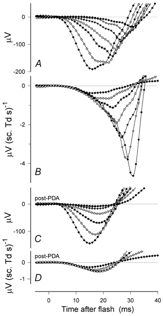
Figure 4. Isolated rod-driven ERG.

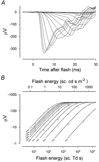
A, records showing the first 30 ms of isolated rod responses obtained with a wide range of stimulus energies (see Fig. 1 for the mixed rod–cone responses from the same session, sm451). B, amplitude of the responses measured at fixed times between 3 and 15 ms after the flash vs. stimulus energy on double-logarithmic scales. Data have been fitted with eqn (1) as an ensemble (i.e. with a common value for V_max) using a Levenberg-Marquardt error minimisation method. Response is initially proportional to stimulus energy but then saturates in a manner intermediate between an exponential and a hyperbolic function (eqn (1), F= 0.7).

Figure 11. Fits of non-linear model to rod-driven responses.

A, energy-scaled rod-driven responses from macaque XE (Fig. 4) plotted on double-logarithmic axes and fitted with lines generated by a model that included non-linear saturation. The delay and sensitivity parameters were chosen to provide a good fit of the linear kernel of the model to the envelope of the data at early times (< 12 ms) and then V_max was adjusted to give a good fit to the later part of the leading edge of the a-wave. B, same results plotted without energy scaling on semi-logarithmic axes to show the fit of the model at early times. The grey lines show fits of the non-linear rod photoreceptor model described in the text. Parameter values were obtained by fitting data points earlier than 11 ms, and having amplitudes less than 80 % of the peak, as an ensemble using the downhill simplex method of Nelder and Mead to minimise the total unweighted squared error over the data set. Points used for parameter estimation have been left unconnected by black lines. The time scales have not been adjusted to take account of the delay introduced by the low-pass filter of the recording system.

RESULTS

Dark-adapted ERG

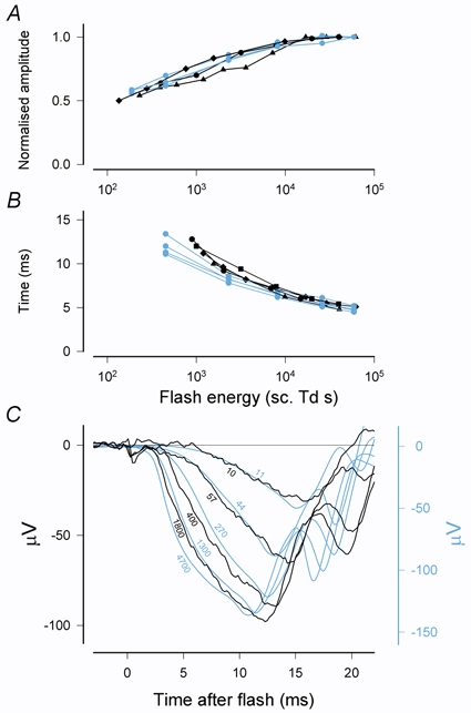
Figure 1A and B shows on an expanded time scale the a-waves of a family of ERG responses, some of which are shown more completely in the inset. These ERGs were obtained from a normal dark-adapted macaque eye in response to brief flashes with luminous energies ranging from 0.37 to 59 000 sc. Td s (i.e. about 4.6 × 10⁵ to 7.4 × 10⁵R* per rod). Although these responses represent combinations of signals from both rods and cones as well as from various postreceptoral cells, the leading edge can be reasonably well fitted (as shown by the grey lines in Fig. 1B) by the simple model originally proposed by Lamb & Pugh (1992) to account for the initial time course of the photocurrent generated by amphibian rods and subsequently shown to fit, about as well as in this example, the leading edge of human a-waves (Breton et al. 1994).

Figure 1. Dark-adapted mixed rod-cone ERG.

A, energy of blue flashes in A and B increased from 0.37 to 188 sc. Td s (0.086–43.8 ph. Td s) by factors of 2 in nine steps; the strongest five flashes were white with energies of 450, 2300, 8200, 26000 and 59000 sc. Td s (270, 1300, 4700, 14800, 33500 ph. Td s). The inset shows selected responses on a longer time scale so that the whole ERG can be viewed. B, the early part of records fitted with a simple delayed Gaussian model of the leading edge of rod photoresponses (Lamb & Pugh, 1992; Breton et al. 1994). (Subject: XE; session: sm451.)

It might be supposed that the slight failures of the model that can be seen at very early times for the strongest stimuli and at later times for the weakest stimuli are related to the composite nature of the mixed rod-cone ERG. However, most recent studies of the human a-wave (e.g. Hood & Birch, 1990a,b, 1993, 1995; Cideciyan & Jacobson, 1993, 1996; Smith & Lamb, 1997; Friedburg et al. 2001) in which various methods have been used to separate the rod- and cone-driven ERGs, have found that even when the rod and cone a-waves are considered separately, the fit of the model can be improved by some modifications to Lamb & Pugh's formulation. We now examine the isolated rod- and cone-driven a-waves of the macaque ERG to see if modifications to the basic model can result in further improvements in its descriptive power of these responses.

Isolating rod- and cone-driven components

In order to obtain records of cone-driven ERG responses that were uncontaminated by rod-driven signals we chose an adaptation method that would allow us to record cone-driven responses to both weaker blue stimuli as well as to much stronger white ones. However, because a steady background that is sufficiently strong to suppress all rod activity also has a significant adapting effect on cone-driven responses (even though it may have little effect on the cones themselves), we adopted a transient rod-saturation procedure similar in principle to that used by Nusinowitz et al. (1995) and Friedburg et al. (2001). In our procedure the test stimulus was delivered 300 ms after turning off a blue adapting light of 2500 sc. Td (∼470 ph. Td) that had been kept on for 1 s. Although preliminary probe-flash experiments (not illustrated) had shown that a light with this retinal illuminance and duration fully saturates all the rods for at least 0.5 s after the light is extinguished, it was important to determine whether or not the sensitivity of the cone system would fully recover within this time.

Isolated cone-driven ERG

Figure 2 shows responses to a flash of 44 ph. Td s (188 sc. Td s) that was delivered at various times with respect to the extinction of the adapting light (from 200 ms before the light was turned off to 700 ms after it was turned off). Although in the fully dark-adapted state this stimulus produced an a-wave of 270 μV amplitude, at all times illustrated here the amplitude was much reduced by the adapting light. While the background was still on (record labelled −200 ms) the amplitude of the a-wave was reduced to 40 μV but it recovered to ∼100 μV shortly (100 ms) after the background was turned off and remained unchanged at the later times of 400 and 700 ms.

Figure 2. Isolating the cone-driven response.

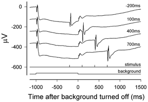
Responses to a blue test flash of 44 ph. Td s (188 sc. Td s) presented at different times relative to a rod-saturating background of 2500 sc. Td that was on for 1 s in every 3 s. The top trace shows the response to a test flash delivered 800 ms after turning the background on (i.e. −200 ms relative to turning it off). The next traces show, successively, responses to flashes delivered 100, 400 and 700 ms after turning the background off. (XE, sm465.) The dark-adapted response to the same stimulus can be seen in Fig. 1 for the same animal recorded in another session.

This effect can be more clearly seen in Fig. 3A which shows responses obtained at the different times superimposed on a faster time scale, for flashes of 5.5 ph. Td s (top records), 44 ph. Td s (middle) and 34 000 ph. Td s (bottom). By 100 ms after extinction of the background, the leading edge of the a-wave had already recovered to exactly the same size as it would after 400 or 700 ms, although later portions of the response still changed a little between 100 and 400 ms. These results indicate that for the leading edge at least, it is not necessary to wait longer than 100 ms after extinction of a background of this luminance and duration to obtain effectively dark-adapted cone-driven responses. However, to provide a margin of safety, the test stimulus was normally delivered 300 ms after the background was turned off. By this time the transient response elicited by extinguishing the background had subsided sufficiently to make it unnecessary to subtract the response to the background alone from that to the test stimulus and background combined.

Figure 3. Isolated cone-driven responses.

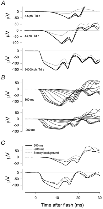
A, responses to a blue test flash of 5.5 ph. Td s (top records), a blue test flash of 44 ph. Td s (middle records) and a white flash of 34 000 ph. Td s (bottom records) delivered 800 ms after turning on a rod-saturating background (thin line) or 100, 400 or 700 ms after turning it off. Dark-adapted responses to the same stimuli can be seen in Fig. 1. (XE, sm465.) B, families of responses to flashes of different energies delivered either 300 ms after turning off the background that was on for 1 s in every 3 s (top records) or 800 ms after turning it on (i.e. −200 ms relative to turning off the background; bottom records). Flash energies were 5.5, 11, 22, 44, 270, 1300, 4700, 4700, 15 000, 34 000 ph. Td s (24–59 000 sc. Td s) (ZE, sm468.) C, responses to a blue test flash of 5.5 ph. Td s (top records) and a white flash of 34000 ph. Td s (bottom records) delivered 300 ms after turning the background off (thick line), 800 ms after turning the background on (i.e. −200 ms relative to turning off the background; thin line) or presented on a continuous background (dashed line). (ZE, sm468.)

Figure 3B shows sets of responses to a wide range, 6000: 1, of stimulus energies applied either 200 ms before (bottom set) or 300 ms after (top set) extinguishing the rod-suppressing background for a different animal (ZE). As was observed in Fig. 3A, for all three animals that we studied in this way, the amplitude of the a-wave evoked by all but the weakest stimuli increased by ∼30–60 μV after the background was turned off. This was largely the result of a continued slow rise towards the peak that was much reduced, or absent in some cases, while the background was on. In Fig. 3B, while the background was on, the records either reached a plateau (after ∼5 ms with the strongest stimuli) or were obviously levelling off well before they were interrupted by the later positive-going components. After the background had been turned off the records all approached approximately the same steady slope as they progressed towards the a-wave peak. Our interpretation of the slow rise as a negative postreceptoral component that is more easily adapted than the cone photocurrent will be discussed later.

Because it is well known that the amplitude of both the a-wave and the b-wave of the photopic ERG continues to grow for some time after the initial reduction produced by turning on an adapting background (Peachey et al. 1989; Murayama & Sieving, 1992), we also compared responses to test stimuli delivered after extinguishing the background with ones recorded while a steady background of the same luminance was on for at least 15–20 min. Figure 3C shows typical cone-driven responses obtained 300 ms after turning off a background of 2500 sc. Td together with responses recorded 800 ms after turning on the background, as well as responses recorded after the background had remained on for 15–20 min. Although in each of the three animals we observed some recovery of the amplitude of the leading edge of the cone-driven a-wave when the background remained on for the longer time, and in some cases it was more than that illustrated in Fig. 3C, this never grew to be as large as it rapidly became after turning the background off.

As a result of these observations we concluded that cone-driven signals recorded shortly after turning off a rod-suppressing background provide a better indication of the cone-driven component of the mixed rod- and cone-driven dark-adapted ERG than recordings made using a continuous adapting background, even if it is on long enough for responses to grow to full amplitude. A further advantage of isolating the rod-driven response by subtraction of two ERGS evoked by exactly the same stimulus is that the early receptor potential and any stimulus artefact are cancelled from the resulting rod-driven ERG.

Isolated rod-driven ERG

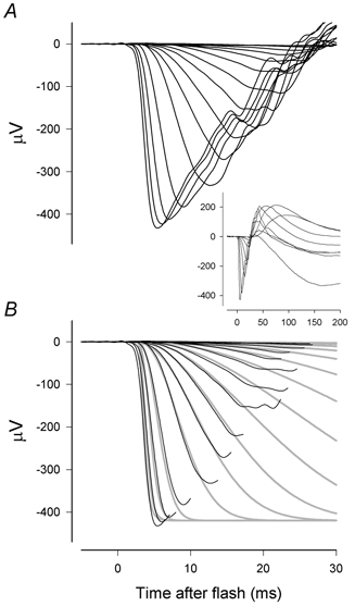
Figure 4A shows the first 30 ms of a typical set of isolated rod-driven ERGs obtained with the same wide range of stimulus energies shown in Fig. 1. While the peak a-wave amplitudes in response to strong stimuli are less than in the mixed rod-cone ERG, the records do not look very different from the mixed ERGs from which they were derived (Fig. 1A). However, inspection of records obtained with weaker stimuli that give rise to a-wave amplitudes of no more than about one-third the maximum shows a rapid downward acceleration that starts a few milliseconds before the a-wave peak, making the peak more prominent than it otherwise would be. While this feature is presumably also present in the mixed records, in those records it is obscured by the onset of early cone-driven oscillatory potentials (as seen in records in Fig. 3B after about the first 10 ms).

It is clear from Fig. 4A that the rod-driven a-wave is a complex non-linear response. Not only does the peak amplitude approach some saturated value as the stimulus energy is increased, but the time course of the wave changes. In particular, the time-to-peak and the time to the first zero-crossing are not constant and independent of stimulus energy as they would be if the responses were generated entirely by a linear system or any simple system with a static non-linearity. Thus any model that describes the curves in full would have to include either intrinsically time-dependent non-linearities or involve summing the outputs of multiple parallel systems with static non-linearities. Because it is not immediately practicable to devise such a model, initially the aim of explaining the leading edge of the a-wave as the response of a single system remains more appropriate.

Several studies (following Hood & Birch, 1990a,b) have adopted such an aim and have applied models originally developed to describe the responses of functionally isolated rods (e.g. Baylor et al. 1984) to the leading edge of the rod-driven a-wave. Such models all suppose that the rod response is in effect generated by applying a slightly delayed signal proportional to the light as the input to a low-pass filter that is followed by a static non-linearity, though Lamb & Pugh (1992) derived their equivalent model from a rather different perspective. All these models take as a starting point that when the ERG amplitude is small it is proportional to the stimulus energy and its waveform is invariant with respect to the energy.

A simple way to demonstrate that this initial proportionality between response amplitude and stimulus energy applies to the rod-driven a-wave is to plot the amplitude measured at fixed times vs. stimulus energy on double-logarithmic scales. The result of doing this at times between 3 and 15 ms after the stimulus is shown in Fig. 4B for the responses of Fig. 4A. At times later than about 5 ms, the amplitude rises with energy to a peak before declining, and thus for clarity, data points in Fig. 4B for energies greater than those giving the maximum response have been omitted. This makes it easier to see that, for each measurement time, amplitudes below the maximum lie close to a single function of stimulus energy that has been appropriately shifted horizontally to fit each data set. The function used here is intermediate between an exponential and a hyperbolic function:

(1)

where V_t is the ERG voltage at time t, V_max is the maximum voltage, E is the stimulus energy, k_t is the responsivity at time t and F is a constant between 0 and 1. In this case F was set to 0.7 (see later) and the lines were fitted as an ensemble using the Levenberg-Marquardt error minimisation method with the data points all equally weighted.

Measurements of responsivity (as just defined) allow us to assemble information about the time course of the linear processes underlying the rod-driven ERG responses to stimuli with widely varying energies and so obtain a good description of how the output of the hypothesised linear filter increases at early times (as originally suggested by Baylor et al. 1974). Figure 5A shows on double-logarithmic axes the estimates of rod responsivity obtained from the fits of the curves in Fig. 4B as a function of time (3–15 ms, open circles). Similar measurements are shown (open symbols) for two other macaques, one of which (triangles, animal DE) was tested on two separate occasions and provided measurements as early as 2 ms after the stimulus flash. The filled circles are plots of the numerical results of an analysis of a single human ERG (presented in legends to Fig. 1 and Fig. 2 of Friedburg et al. 2001) made in essentially the same way. In this figure, as well as in Fig. 6 and Fig. 9, the time scale has been adjusted to take account of the small delay introduced by the low-pass filters used to limit the bandwidth of the signal prior to its digitisation. This adjustment makes it possible to compare directly the time course of the macaque and human responsivity functions which were recorded with different low-pass filters.

Figure 5. Rod responsivity at early times.

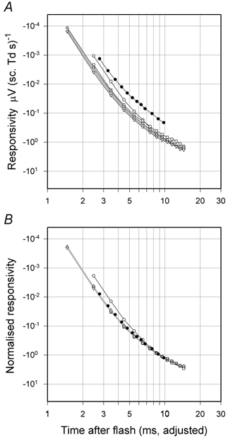
A, shown on double-logarithmic axes (open circles) are the estimates of rod responsivity obtained from the fits of the curves in Fig. 4B as a function of time (3–15 ms). Similar measurements (open symbols) made on two other macaques one of which (DE, triangles) was tested on two separate occasions (sm466 and sm469). The filled circles are for a single human ERG (TDL, data from Friedburg et al. 2001). B, plots from A arbitrarily normalised to unity at 9 ms after the flash. In both A and B the time has been adjusted to take account of the group delay of the recording filter (0.53 ms for the macaques and 0.23 ms for human). The grey line is drawn through the means of the two sets of readings from macaque DE.

Figure 6. Energy-scaled rod a-wave.

Rod a-wave records for macaque DE (similar to those of Fig. 4A) have been scaled by stimulus energy and replotted on the same double-logarithmic axes as Fig. 5A. The figure also contains a replot of the curve from Fig. 5 with interpolated responsivity values for the same macaque. As in Fig. 5 the time scale has been adjusted to take account of delay introduced by the low-pass filter of the recording system. Responses generated by LED pulses were subject to small corrections at early times to take account of the stimulus duration. This was done by assuming that the effect of stimulus duration would be the same on the recordings as it was calculated to be for the model that was subsequently fitted to the data.

Figure 9. Linear model of rod photoresponse.

A linear model as described in the text was fitted to isolated rod a-wave responsivity vs. time for one animal (DE), two sessions averaged, and plotted on double-logarithmic axes (sm466 and sm469). The continuous grey line shows the linear responses of a model with the following parameters: delay 3.35 ms of order n= 13, phototransduction time constants 30, 70 and 150 ms. The delay, the value of n and a sensitivity parameter were adjusted to provide a good fit by eye to the first 12 ms of the data. The dashed grey line is the prediction of a model that includes a positive PII component that is generated as the third integral of the response predicted by the rod model. The relative responsivity of the PII component is set to a value that results in the rod and PII responses summing to zero at 24 ms after the flash, a typical time for the zero crossing obtained after blocking all postreceptoral responses other than those of ON bipolar cells (see Fig. 10B for an example). The time scale has been adjusted to take account of the group delay of 0.53 ms introduced by the low-pass filter of the recording system.

While there was variation between individual macaques in the magnitude of their responses (and an even bigger difference for the human), the time courses of the responses in Fig. 5A during the first 10–15 ms of the rod a-waves were all very similar. This is more obvious in Fig. 5B where each plot has arbitrarily been normalised to unity at 9 ms after the flash. Results from two of the macaques and the human are essentially identical while results from the third macaque are just slightly more delayed. Although we shall later consider mathematical formulations of the time course of the early responses, the grey lines in Fig. 5A and B are simply a cubic-spline interpolation of the geometric means of the two separate sets of data from macaque DE. These data fall on a smooth curve whose log-log slope becomes progressively less at later times, ranging from about −6 at 2 ms to −2 at 12–15 ms after the flash.

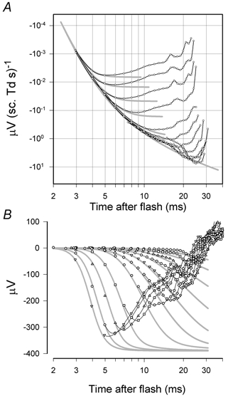
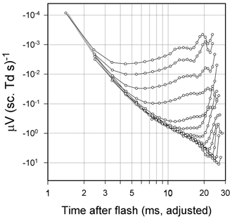
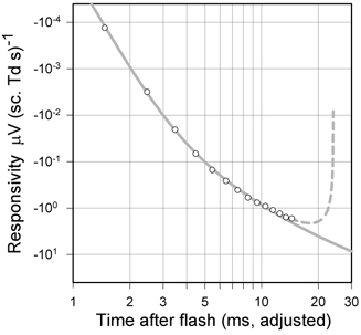
A simpler way to see how responsivity varies with time while also examining the limits of the range of linear operation is to superimpose on a single plot energy-scaled versions of the rod ERG records obtained with stimuli of various energies. To illustrate this, Fig. 6 and Fig. 7B are energy-scaled replots of the a-waves of Fig. 4A and Fig. 7A. Whereas Fig. 7B shows the data on linear axes, Fig. 6 uses the logarithmic co-ordinates of Fig. 5B and has copied to it the curve from Fig. 5B with interpolated responsivity values for macaque DE. In Fig. 6, the earliest part of each energy-scaled record falls along a common line that corresponds closely to the responsivity curve. However, at later times, each record falls away from the common envelope as the response saturates.

Figure 7. ERG responses to seven stimuli of energies increasing by factors of two from 7.9 to 509 sc. Td s.

A, rod-driven ERG obtained after subtracting cone-driven responses from mixed rod-cone ERG (not shown). B, replot of the records in A scaled by stimulus energy. C, responses to the same range of stimulus energies after intravitreal injection of PDA (4 mm). D, replot of the records in C scaled by stimulus energy. (NI, sm404.)

The records for the higher-energy stimuli (the upper six or seven records in Fig. 6 and the upper three in Fig. 7B) have a different appearance from those obtained with lower stimulus energies. These records break away from the common envelope gradually and show a relatively flat maximum whereas the lower-energy records deviate more abruptly from the common envelope and show an exaggerated, sharper peak. This change in the form of the records occurs around 15 ms after the stimulus and, as indicated in experiments with intravitreal pharmacological agents below, probably reflects negative contributions from postreceptoral cells whose responses grow to exceed those of the rods at later times but saturate at a lower level.

Postreceptoral contributions to the rod-driven a-wave

Although it is generally supposed that the positive-going signal from depolarising (ON) bipolar cells is primarily involved in determining the time of the a-wave peak, it is likely that early contributions from other postreceptoral cells also influence the peak, at least at lower stimulus energies. To investigate this we examined the effects of suppressing the light-evoked activity of most postreceptoral cells (except depolarising bipolar cells that possess metabotropic, mGluR6, receptors) by blocking synaptic transmission involving ionotropic glutamate receptors with the non-specific glutamate analogue PDA injected into the vitreous chamber.

Control ERGs illustrated in Fig. 7A and B show, respectively, isolated rod-driven ERG records and energy-scaled versions of the same records. Responses are shown to seven stimuli with energies increasing by factors of two from 7.9 to 509 sc. Td s. All stimuli produced responses small enough to be in the linear range of operation for at least the first 10 ms (as indicated by the superposition of the energy-scaled records in B), while being large enough to give reasonably noise-free records. In the control condition, the late negative peak characteristic of low amplitude rod-driven a-waves (e.g. Fig. 6) can be seen in the unscaled records of Fig. 7A, and it becomes prominent in the energy-scaled records (Fig. 7B). Also seen in the energy-scaled records of Fig. 7B is that the leading edges of the a-waves all closely conform to a common envelope nearly up to the time of the prominent peak. However, the trailing edges are widely separated and there is a steady reduction in the time to the first zero-crossing as stimulus energy is increased (upper records). This indicates that the mechanisms contributing to the later part of the a-wave are operating in a very non-linear manner.

Figure 7C and D shows the equivalent records for the same eye after injection of PDA. Figure 7D shows responses to only the four strongest stimuli. Although PDA reduced the a-wave amplitude for all stimulus energies (compare Fig. 7A with 7C), the effect, which was also seen in similar experiments in four other animals, was particularly marked for the lower amplitude a-waves. Also over a substantial range of low-energy stimuli (i.e. up to about 100 sc. Td s), PDA made the time course of the a-wave invariant with stimulus energy, giving it a constant time-to-peak of about 19 ms (considerably shorter than in the control records), a constant time to the first zero crossing of about 25 ms and a constant energy-scaled amplitude (see Fig. 7D and also Fig. 10B). This implies that there is a substantial range of stimulus energies over which the isolated rod photocurrent and rod (or rod-driven ON) bipolar cell components are effectively generated by linear mechanisms (at least for the first 25 ms of their response). Jamison et al. (2001), in similar experiments found that PDA increased the peak amplitude of the a-wave slightly, but did not observe the constant time of zero-crossing, suggesting a smaller effect of PDA in their experiments. We show below that the pharmacologically isolated a-waves that we found after PDA can be described by a simple model that combines responses of rods and rod-bipolar cells.

Figure 10. Effect of pharmacological suppression of postreceptoral responses.

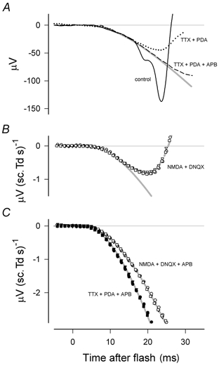
A, superimposed unscaled responses to a flash of 19.8 sc. Td s both before administering any drug (continuous black line) as well as after injecting TTX and PDA (dotted line) and then APB (dashed line) (SN, sm241). The continuous grey line was generated by fitting the linear rod model described in the text. B, energy-scaled responses following intravitreal injection of NMDA and DNQX to block all postreceptoral activity other than that of ON bipolar cells (ES, sm188). The dashed grey line is the sum of the linear responses of models of rod photoreceptors and ON bipolar cells (see text and Fig. 9). The continuous grey line shows the modelled photoreceptor response alone. Flash energies were 16, 32 and 64 sc. Td s. C, energy-scaled responses of two animals following intravitreal injections of NMDA, DNQX and APB (ES, sm188, open symbols) or TTX, PDA and APB (SN, sm241, filled symbols). Grey lines are linear responses of the rod photoreceptor model described in the text; parameters were chosen to give the best fit by eye. Flash energies for sm241 were 4.5, 8.9 and 19.8 sc. Td s.

Modelling the rod response

It is generally accepted that the early part of the photocurrents of isolated photoreceptors can be described by a model in which a static saturating non-linearity follows several linear dynamical elements (e.g. Penn & Hagins, 1972; Baylor et al. 1974; Lamb & Pugh, 1992). By extension, it has been supposed that the photocurrent-related component of the ERG recorded from the whole isolated retina or the intact eye can be modelled by assuming that the photocurrent (slightly modified by a linear low-pass filter related to the photoreceptor membrane capacitance) is linearly converted to a voltage as it flows through a resistive extracellular path in the retina (e.g. Penn & Hagins, 1972; Hood & Birch, 1990a,b; Smith & Lamb, 1997). Thus, we can describe the time course of the photocurrent-related ERG responses by a linear model so long as their amplitude remains small enough for saturating non-linearities to be unimportant. A good linear model of this kind may provide useful information about the linear elements involved.

The linear model that we have chosen (e.g. to generate the curve in Fig. 9), incorporates many of the features of models previously proposed to account for either the rod photocurrents or the ERG a-wave. The model is a cascade of several stages whose overall effect on an input signal is calculated by successively convolving this signal with the impulse response of each stage. In practice we have done this numerically using signal and response functions sampled at 20 μs intervals. When the model is used only to account for small-signal linear behaviour it does not matter in what order the convolutions are performed. However, when we subsequently modify the model to include the saturating non-linearity, it will be important that the dynamical elements are correctly placed before or after the non-linearity.

In common with previous models we incorporate a short delay which we have chosen to formulate as a cascade of many exponential delays with equal time constants. The impulse response of such a composite delay is:

(2)

where the order of the filter (n) is an integer equal to the number of stages and τ_d is the total delay time. The form of this function is shown in Fig. 8A for values of n between 1 and 14. For n around 12 (a typical value we found to fit the very early part of the rod a-wave), the function has returned to close to zero at roughly twice the delay time, indicating that approximating this composite delay by a transport delay of about 2.5 to 3.5 ms, as in some previous models, would produce significant differences at times less than 6 or 7 ms after the flash. For purposes of curve fitting it is convenient to use a delay function with continuous parameters of the form:

(3)

where the factorial is replaced by a gamma function. For integer values of n this reduces to eqn (1).

Figure 8. Rod photoreceptor model functions.

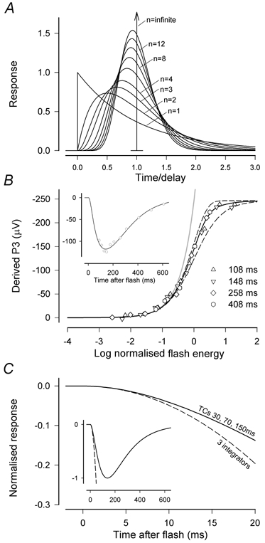
A, impulse response of the delay function described by eqn (2). When n becomes very large the function approaches an impulse at time 1, equivalent to an ideal transport delay. The form of this function for values of n between 1 and 14 is shown in diagram. B, the derived rod response to test flashes covering a range of energies at 108, 148, 258 and 408 ms estimated using a saturating probe-flash procedure. The probe flash had an energy of 15 000 sc. Td s and responses were measured 8 ms after it was delivered. The data were first fitted as an ensemble with a saturating function intermediate between an exponential and a hyperbolic function (eqn (1) with F= 0.7) to provide a single value for the maximum response and a responsivity constant for each time. The responsivity constants were then used to normalise the data for each time to obtain the superimposed values that are plotted. The continuous line shows the model fit for F= 0.7 while the dashed lines show the exponential and hyperbolic functions (F= 1 and F= 0, respectively). The inset shows measurements of the derived rod response at various times after a test flash of 2.5 sc. Td s. The line is the response of a model having a delay of 3.0 ms, a three-stage filter with time constants of 30, 70 and 150 ms and a saturating non-linearity intermediate between an exponential and a hyperbolic function (eqn (1) with F= 0.7). (XE, sm410.) C, comparison of the time course of the normalised linear impulse response using two different formulations, one that includes three integrations (Lamb & Pugh, 1992), and one that contains the three time constants (TCs) estimated from saturating probe-flash measurements of the later time course of the rod photocurrent as in B. Inset shows the same comparison on reduced scales to show the entire time course of the impulse response.

Although the delay is often described (as we have just done) as though it precedes the transduction process, it is not necessary that this be the case. In reality, the delay may relate to a later mechanism or process or result from the combination of several shorter delays occurring at different points in the cascade. However, as far as modelling is concerned the only requirement is that it should be operative prior to the non-linearity (this is not necessary for a transport delay).

Following Lamb & Pugh's (1992) analysis of the kinetics of the rod transduction cascade that characterised the three major biochemical stages of the cascade as integrators, most models of the leading edge of the rod response have been based on this formulation. However, earlier descriptive models that were intended to apply to the complete waveform of the rod's response and not just the initial portion (e.g. Penn & Hagins 1972; Baylor et al. 1984) had suggested that the waveform was shaped by four or more cascaded low-pass filter elements that acted as ‘leaky’ integrators, having time constants for which various values were proposed. To resolve the apparent contradiction in these results (which may be partly explained by the absence of any explicit delay in the earlier models), we examined the time course of derived rod responses in macaques (see inset to Fig. 8B for an example) using the rod-saturating probe-flash procedure of Pepperberg et al. (1997). Although in macaques this technique did not provide good measurements of the response at times much earlier than the peak, which occurred at 138 ± 11 ms (n= 6), the later part of the response was adequately modelled as the slightly delayed (3 ms) output of a three-stage low-pass filter (with time constants of 30, 70 and 150 ms) that was followed by a saturating non-linearity intermediate between exponential and hyperbolic. Thus, taking into account Lamb & Pugh's (1992) theoretical arguments and our ability to fit the later part of the derived rod response with a model of this kind, we incorporated a three-stage low-pass filter with these representative time constants into a model primarily intended to describe the leading edge of the a-wave.

The impulse response of the main transduction cascade that is represented by the three-stage filter is described by:

(4)

where the convolution operation is represented by * and τ₁, τ₂ and τ₃ are 30, 70 and 150 ms (though this is not to imply that the time constants of the three successive biochemical stages are necessarily in this order).

Our decision to incorporate a three-stage filter with relatively short time constants, rather than three ideal integrators with infinite time constants, was partly to be able to account for the complete time course of the rod response and partly because simple simulations showed that the difference between the impulse response of the three-stage low-pass filter with these time constants and that of three cascaded ideal integrators (Lamb & Pugh's model) became significant at times relevant to the present study. To illustrate this, Fig. 8C compares the linear impulse responses of these two candidate models for the major stages of the transduction cascade and shows that the difference becomes detectable at times longer than about 5 ms. The inset shows the entire time course of the responses. When the delay that is common to both models is included, this would become 8 or 9 ms after the stimulus.

Having obtained expressions for the impulse response functions of the delay and transduction stages we now can calculate the waveform of the output from the transduction mechanism (O_transducer) in response to any arbitrary light input with time course Φ(t), by convolving this function with the impulse response functions of the delay and the transduction cascade:

(5)

where k is a responsivity constant. In practice the duration of the stimulus flash was ignored (i.e. the waveform was assumed to be a delta function) if the duration was less than 128 μs, as it was for all xenon flashes. For longer flashes generated by the LEDs, Φ(t) was a rectangular pulse whose time course was explicitly incorporated into the computations.

There are two more elements whose effects must be considered in computing the waveform of the electrical signal (V_record (t)) that is recorded in response to a light stimulus, even if the signal from the transduction mechanism is small enough for the saturating non-linearity to be ignored. These elements are: the electrical filter formed by the capacitances of the cell membranes of the photoreceptor inner and outer segments together with the resistances of the associated intra- and extracellular current paths, and any low-pass electrical filter used in the recording system to limit the bandwidth of the signals. If the ‘membrane filter’ is assumed to have the characteristics of a single-stage low-pass filter (a rough approximation; see Penn & Hagins, 1972) then its impulse response function will be an exponential as also will be that of the simple low-pass recording filter, such as used in our own system.

Thus the final recorded output can be computed as:

(6)

where, in our experiments, τ_amplifier is 0.53 ms (corresponding to a corner frequency of 300 Hz).

Model fits to experimental data in the linear range

Since τ_membrane is probably much less than 1 ms (see Penn & Hagins, 1972), we cannot expect to differentiate its effect from that of the many notional elements making up the delay for responses in the linear range. Therefore we have not treated it as a separate element when adjusting the parameters of our linear model to fit the experimental measurements. Thus, with the time constants of the cascade set to the values given above, the linear model has only three free parameters, the duration of the delay (τ_d), the order of the delay (n), and the responsivity constant (k).

Figure 9 shows that a good fit to the measurements can be achieved when the three free parameters are adjusted to match the model to the data over the range 2–12 ms. While the fit is very good up to about 10 or 11 ms, there is indication of a small but systematic divergence at the longest times (between 10 and 15 ms) where the data lie above the model curve.

The a-wave after blocking inner-retinal and hyperpolarising bipolar cells

In this section we consider, as did Jamison et al. (2001), whether the model that describes the first 10–12 ms of the energy-scaled a-wave can also satisfactorily describe any later part of the rod response when this is revealed by pharmacologically suppressing the contributions of all postreceptoral cells. Figure 10A shows responses of one animal to a flash of 19.8 sc. Td s before administering any drug (continuous line), after injecting TTX and PDA (dotted line) and then after APB had been added (dashed line). Although the drugs had a profound effect on the later part of the a-wave, in neither case was there any specific effect on the early part of the leading edge which was well fitted up to about 15 ms in this example by our rod-response model (grey line). The effect of TTX and PDA, which blocked all postreceptoral activity except that of depolarising bipolar cells, was particularly dramatic, changing the initial negative deviation of the control a-wave from the model line into a positive deviation. A similar effect was obtained in another animal with a mixture of NMDA and DNQX and this is shown by the energy-scaled plots of Fig. 10B. These plots also illustrate how the summed linear responses of rods and rod-bipolar cells can be described by adding the output of a simple rod-bipolar cell model that is described below to that of our rod model (dashed grey line).

After injecting APB to block depolarising rod-bipolar cells as well, the leading edge of the a-wave followed the modelled rod photoreceptor line for a longer time. This can be seen by comparing the black dashed line with the continuous grey line in Fig. 10A or the data points from the two animals with the grey model lines in the energy-scaled plots of Fig. 10C. Although blocking all postreceptoral responses resulted in an a-wave that was well described by the rod model out to about 25 ms, at longer times the ERG (e.g. Fig. 10A) still turned upward as has been observed in other studies in which postreceptoral responses were blocked (e.g. Kang Derwent & Linsenmeier, 2001).

A model for the leading edge of PII

To estimate more quantitatively the magnitude of the relative contributions made to the rod-driven a-wave by the rods and the rod-bipolar cells (or, perhaps for stronger stimuli, by rod-driven depolarising cone-bipolar cells) we examined in more detail post-PDA (or post-NMDA/ DNQX) rod-driven a-waves as illustrated in Fig. 10B. These we fitted with a linear model of the kind that was developed to describe similar results from cat (Robson & Frishman, 1996). This model was based on the finding that the initial part of the leading edge of the ERG response of cat rod-bipolar cells (termed ‘PII’) is well described as a signal that initially rises after a short delay as the fifth power of time (Robson & Frishman, 1995), a time course that can be explained by the existence of a G-protein cascade in the bipolar cell with similar kinetics to the cascade in rods. On this basis it was supposed that PII would rise as the third integral of the rod response in the same way as the rod response was thought to rise as the third integral of the light stimulus. While a three-stage filter with finite time constants might be expected to provide a better model of the process generating PII than three integrators, we do not yet know what these time constants might be. We have therefore retained the triple integration of the rod signal as an approximation to the early part of the bipolar cell response that could be added to the rod response to obtain the complete ERG. The relative amplitudes of the rod and rod-bipolar cell components were adjusted to sum to zero at 24 ms, the experimentally determined time of the first zero crossing of responses in the linear range. The dashed grey line in Fig. 10B, and that in Fig. 9, shows the modelled sum of the photoreceptor and rod-bipolar cell responses; the continuous grey line plots the rod component alone.

The satisfactory fit to the data of the dashed grey line in Fig. 10B supports our use of this rather simple model. From the model we can estimate the relative contributions of rods and rod-bipolar cells to the a-wave at different times after the stimulus. While there is no exact time at which PII commences, the model indicates that PII has grown to be 5 % of the photoreceptor signal at 11.5 ms and 10 % at 14.3 ms. If the response of depolarising rod-bipolar cells has become of significant magnitude by about 13 ms after the flash (where it is about 8 % of the photoreceptor signal) it is possible that the predominantly negative signals seen in the rod-driven ERG after about 15 ms (e.g. Fig. 10A) could be generated by inner-retinal cells of the ON-pathway that are synaptically activated by these bipolar cells.

Modelling the non-linear responses of the rods

As well as using the rod-saturating probe-flash procedure to examine the time course of the derived rod response we also examined the amplitude-energy relation near the peak at times when the response was quite large. An example for an animal in which measurements were made at several different times is shown in Fig. 8B. In all cases the relationship was slightly less abrupt than an exponential function and slightly more abrupt than a hyperbolic function (both of which are linear at low levels). In this, as in the four other animals we examined, a satisfactory fit was provided by an intermediate curve as given by eqn (1) with F= 0.7 and we have adopted this formulation to describe the saturation at earlier times as well.

Thus, to calculate the time course of rod responses to stronger stimuli than those for which the behaviour is linear, the transducer output is assumed to be subject to a static saturating non-linearity that is a weighted combination of exponential and hyperbolic saturating functions. Specifically, O_transducer in eqn (6) is replaced by:

where O_max is the amplitude of the saturated output and F is set to 0.7.

A set of energy-scaled rod-driven responses from macaque XE fitted with lines generated by this model and plotted on double-logarithmic axes is shown in Fig. 11A while Fig. 11B shows results plotted without energy scaling on semi-logarithmic axes to demonstrate the good fit of the model at early times. Adjustment of the four free parameters of this model (the three needed for the linear kernel of the model together with a fourth that determines the saturation level) provides an excellent description of the set of responses nearly up to the peak when the stimuli are of high energy and the peak occurs earlier than 10 ms, and for the first 10 to 12 ms when the stimulus energy is lower. There was no obvious discrepancy between the model and the experimental results that made it necessary to invoke any significant ‘membrane filter’ operating after the non-linearity or any other non-linearity than the one already postulated.

To obtain more insight into the good fit achieved without a ‘membrane filter’ after the non-linearity, we refitted the data with a model that explicitly included a single-stage filter at the output. The optimum value for the time constant of this filter was always less than 0.2 ms and including the filter produced a negligible improvement in the fit. If the time constant was forced to be 1 ms (e.g. Smith & Lamb, 1997) the fit was not quite as good, although it could be improved by allowing the value of F to be increased to 1 (i.e. by assuming an exponential saturation function).

Cone-driven responses

We now consider how to model the cone-driven a-waves, recalling that when these were recorded shortly after a rod-suppressing background had been turned off (Fig. 3B) they included a slowly rising component in addition to the faster-settling component more characteristic of the records obtained while the background was still on. These differences are clearly seen in Fig. 12A and B, which shows another family of responses to stimuli of different strengths applied either 300 ms after the rod-saturating adapting background was turned off or 800 ms after it was turned on. As noted earlier, the slow rise in records after the background was turned off attained about the same limiting slope (prior to the sudden upturn after about 10–15 ms) with the weakest stimuli as it did with the strongest and it was suggested that this slow component originated from postreceptoral cells. We now tested this by examining the effect on the slow rise of intravitreal injection of pharmacological agents that would block postreceptoral activity.

Figure 12. Cone-driven receptoral and postreceptoral responses.

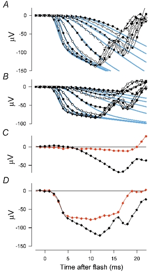
A, responses to stimuli of different strengths (blue: 6.9, 13.7, 27.4, 55 and white: 270, 1300, 4740, 14800, 33600 ph. Td s) all applied 300 ms after a rod-saturating adapting light was turned off. B, responses to the same set of stimuli delivered 800 ms after the adapting light was turned on. The blue lines show fits of the model described in the text that combines the response of cone photoreceptors with a postreceptoral response generated as the integral of the cone response. (XE, sm451.) C and D, pairs of responses to stimuli with energies near the extremes of the families shown in A and B before (black symbols and lines) and after (red) administration of PDA. (XE, sm409.)

Figure 12C and D shows pairs of responses to stimuli of two energies (the stimuli giving records with filled triangles in Fig. 12A and B) delivered 300 ms after turning off a rod-suppressing background before (black records) and after administration of PDA (red records). The leading edges of the control responses in Fig. 12C and D display the same characteristic time course as those of Fig. 12A. In contrast, the response to the highest energy stimulus after PDA showed no sign of a steady rise in voltage preceding its abrupt upturn at 16 ms, and may even have slightly declined before this time. With the weaker stimulus (Fig. 12C) the slowly increasing response seen in the control record was very attenuated by PDA and the final slope before the upturn was essentially abolished. The leading edges of the post-PDA responses resembled those obtained with the background light on (Fig. 12B). However, there were some differences between the effects of the background and PDA, mainly later in the responses; in particular, the responses on the background, but not after PDA, continued to grow, albeit slowly, up to the sudden change to a positive slope. In addition, PDA removed the oscillatory potentials (OPs) near the appearance of the b-wave, whereas the adapting background had no clear effect on these potentials. It should be noted here that PDA blocks transmission not only to OFF bipolar cells but also to amacrine and ganglion cells that could be involved in generation of OPs. Taken altogether these observations indicate that the a-wave of the ‘dark-adapted’ cone-driven ERG, recorded as described above, contains a substantial negative postreceptoral component that grows up to the time of the a-wave peak and that, with the strongest stimuli, this component can reach a significant amplitude around 5 ms after the stimulus.

We can obtain some indication of the characteristics of this slower component from the form of the responses. Firstly we note (e.g. Fig. 3, and Fig. 12A and B) that for the strongest stimuli the early rapid rise of the (saturated) a-wave is followed by a later part with an approximately constant slope, though in the presence of the adapting background this can be very shallow. Since the strongest stimuli must have turned off the cone outer-segment current rapidly and completely, we can assume that the signal transmitted from the cones to the postreceptoral cells for these stimuli approximates a step whose amplitude is independent of stimulus energy. Because this input results in a steadily rising output signal (i.e. in the form of a ramp), we can infer that the postreceptoral mechanisms must effectively integrate the signal from the cones on a time scale of at least 10 ms (this being the duration of the ramping portion of the response). However, this would not immediately explain how the much weaker stimuli that produce much smaller responses from the cones give rise to a slow response that builds up to have approximately the same final slope. To account for this we may imagine that transmission from cones to hyperpolarising bipolar cells, or at some even later retinal stage, saturates at a lower input level than that resulting from complete suppression of the cone photocurrent. While this is all speculative, we can easily see if a mechanism of this kind can provide a quantitatively reasonable account of the observed responses.

To generate the receptoral component of the cone-driven ERG, we have used the same model as for the rods (eqns (2)–(6)) with some modification of the parameters. The time constants of the transduction cascade have all been reduced by a factor of four, in line with the relation of the time-to-peak of the responses of isolated macaque cones and rods (Baylor et al. 1984; Schnapf et al. 1990). We have also assumed that for the cones the ‘membrane filter’ effect is significant and have therefore included a filter stage following the saturating non-linearity. The early negative postreceptoral component of the ERG (V_PR) has arbitrarily been assumed to be the result of integrating a signal from the cones proportional to the contribution (V_C) that they make to the ERG up to some limit (V_SAT) at which saturation sets in abruptly; no other delay is incorporated into this pathway. Thus, we can write:

(7)

where K_PR is a constant,V= max (V_C,V_SAT)and t≥ 0.

The recorded cone-driven ERG (V_CD-ERG) is then obtained by adding together the receptoral and postreceptoral contributions and convolving the sum with the impulse response function of the amplifier (a(t)):

(8)

In adjusting the parameters to obtain a satisfactory fit to the data, it was assumed that the delay and filter time constant would not be altered by the adapting conditions. The model provides an acceptable description of at least the first 10 ms of the data in Fig. 12A and B; the only adjustments required to fit the two sets are to the responsivity and saturation levels of the receptoral and postreceptoral mechanisms. The parameters of the model curves are given in the legend to Fig. 12; however, one parameter of particular interest is the time constant of the cone ‘membrane filter’. In every case (3 animals) a value of 1 ms provided a satisfactory fit.

Macaque and human rod- and cone-driven a-waves

Most previous studies that developed descriptive models of the leading edge of the a-wave were undertaken in humans, but the present study in anaesthetised macaques made it possible to examine the effects of intravitreal pharmacological agents and to obtain less noisy recordings. Because the principal use of models of this kind is to aid in interpreting human ERGs and understanding human retinal function, it is reasonable to ask how similar the human and macaque ERGs really are. For the leading edge of the rod a-wave in Fig. 5 the energy-scaled responses from a typical human were extremely similar to those measured in macaque. A further indication of the similarity can be obtained by examining the amplitude and time-to-peak vs. energy relations of rod-driven a-waves as shown in Fig. 13A and B, which compares our measurements on three macaques with published measurements on several normal humans (Cideciyan & Jacobson, 1993; Thomas & Lamb, 1999; Friedburg et al. 2001). The a-wave peak amplitudes (Fig. 13A) have been normalised to their maximum value (absolute amplitudes will depend upon recording methods and eye size) while the times-to-peak (Fig. 13B) have only been adjusted by very small amounts to take account of the different stimulus durations and recording filters in the various studies (see legend to Fig. 13 for details).

Figure 13. Comparison of macaque (blue) and human (black) ERG a-waves.

A, comparison of peak amplitudes of rod-driven a-waves of three macaques (XE, ZE and DE) with published measurements on several normal humans (Cideciyan & Jacobson, 1993; Thomas & Lamb, 1999; Friedburg et al. 2001). a-wave peak amplitudes have been normalised to their maximum value. B, times-to-peak of rod-driven a-waves adjusted by very small amounts to take account of the different stimulus durations and recording filters used in the different studies. Data of Breton et al. (1994) from mixed rod-cone ERGs are also included here. C, cone-driven responses from a macaque (blue) together with a set from a human (NS, data from Paupoo et al. (2000); black). Numbers on the curves are stimulus energies in ph. Td s. Apart from a very small time shift to allow for different recording filters and an arbitrary adjustment of the relative amplitude scales to bring the two sets of records into line, no other adjustments have been made.

It can be seen that not only is there relatively little variability between different individuals, but also there is no consistent difference between macaques and humans except that the time-to-peak for weaker flashes is slightly longer in humans. Although it is not clear what causes this difference in timing, it may reflect differences in the magnitudes of the postreceptoral components relative to the photoreceptor component. In macaques, contributions from rod-driven postreceptoral components become significant within 12–15 ms after the stimulus even when the amplitude is small enough for linear operation. For larger responses (such as those considered here) these components become significant at earlier times.

Cone-driven a-waves

The a-waves of isolated cone-driven ERGs from macaques and humans are also very similar. Figure 13C shows a set of records from a macaque (made using the transient rod-saturation technique) together with a set from a human published by Paupoo et al. (2000). Apart from a very small time shift to allow for different recording filters and an arbitrary adjustment of the relative amplitude scales, no other adjustments were made. The records interdigitate almost as well as if they had come from a single subject, indicating great similarity in the a-waves of macaque and human. The human records were made using a relatively weak blue background (280 sc. Td) and relied upon the residual effect of previous illumination to saturate the rods, making it likely that postreceptoral components were present at close to their dark-adapted level, as in the macaque records. Other human cone-driven a-waves illustrated in Hood & Birch (1993, 1995) show very similar waveforms, including the later slow rise. Those recordings were made using a red flash with subsequent subtraction of the response to a scotopically matched blue flash, another way to isolate the cone-driven a-wave. The cone-driven a-waves that we recorded also have a very similar waveform to those previously recorded from anaesthetised macaques by Jamison et al. (2001) on a background of less than 10³ sc. Td, as illustrated in their Fig. 4 (though there is a factor of 2 error in the time scale in that figure; J. A. Jamison, personal communication).

DISCUSSION

In this paper we have described a study of the a-wave of the ERG of the dark-adapted macaque that has allowed us to define more precisely how far the leading edge of the a-wave reflects simply the photocurrents of the retinal receptors and to provide an improved descriptive model of the waveform of both rod and cone receptor components. Since the recordings we have obtained from anaesthetised macaques are not easily distinguished from those of normal humans, it seems likely that the modified models that we have used to describe our results could equally well be used to describe the leading edge of the rod- and cone a-waves of the human ERG.

Isolating the cone-driven ERG

An important first step in our study was the separation of rod and cone responses. Although there is no doubt that a purely cone-driven (photopic) ERG can be obtained, as it routinely is in clinical practice, by applying a continuous rod-saturating background, it requires careful titration of the background illumination to find a level that will completely suppress the rods without affecting cone-driven responses. While it may be possible to find a background level at which the rods are completely saturated but the cones themselves are minimally affected (e.g. Hood & Birch, 1993), it is not clear that there is any level that will saturate the rods (and hence all rod-driven components) but leave all cone-driven components unaffected. Indeed, given the significance of adaptation in the generation of contrast-related signals from the proximal retina and the requirement for this to function adequately as the transition from rod to cone vision is accomplished, it seems unlikely that there would be any such level.

We therefore adopted a procedure to saturate the rods completely that was similar to that described by Nusinowitz et al. (1995) and Friedburg et al. (2001), except that we used a long pulse of blue light (2500 sc. Td for 1 s) rather than a brief flash of greater energy. We reasoned that the greater integration time of rods compared to cones would make a longer pulse the best way to saturate the rods while stimulating the cones as little as possible. In both cases one relies on identifying a time during which there has been full recovery of the cone-driven ERG components before there is any recovery of the rods, so that responses during this period can be assumed to be from the effectively dark-adapted cone system. As shown in Fig. 2 and Fig. 3A, the period between 100 ms and at least 700 ms after extinguishing the background meets this requirement and the presence in our records of a continued slow rise in the response preceding the peak of the a-wave is a good indication that the more readily adapted postreceptoral component has been adequately recorded. It should be noted that we are convinced that this is a cone-driven component rather than a rod-driven response to scattered light (e.g. Nusinowitz et al. 1995), not only because our ganzfeld completely filled the visual field but also because the gradient of the sloping portion of the response was effectively independent of stimulus energy unlike any kind of rod-driven response. When the cone-driven ERG is to be subtracted from the mixed rod-cone ERG to isolate the rod-driven response, it is clearly desirable that the recorded cone-driven component be as similar as possible to the one in the mixed response.

Early postreceptoral contributions to the cone a-wave

There are at least three reasons for believing that the later slow rise of the cone-driven a-wave reflects a cone-driven, postreceptoral component. (1) For high-energy stimuli the leading edge has a distinctive transition between the early sigmoidal rise and the later almost linear sloping portion of the waveform that commences about 4 ms after the stimulus, strongly suggesting a two-part response. (2) The sloping portion of the waveform was much more affected by background light than the earlier portion, as seen by comparing the two parts of Fig. 3B or Fig. 12A with 12B. A progressive reduction in the sloping portion of the cone-driven a-wave was noted in humans by Paupoo et al. (2000) when the steady background was increased in steps from about 30 to about 1.7 × 10⁴ ph. Td. (3) The strongest support for there being two portions of the cone-driven a-wave is that intravitreal PDA essentially abolished the later slow rise both when the stimulus energy was high and also when it was much lower (Fig. 12C and D). In the latter case PDA almost completely removed the a-wave. Further, in support of the waveform of the post-PDA record being the cone photoreceptor response, suction electrode recordings from cone outer segments show a similar plateau in response to stimuli strong enough to saturate the response (Schnapf et al. 1990).

The effectiveness of PDA in abolishing or greatly reducing the amplitude of the cone-driven a-waves in the macaque has been thoroughly studied previously by Bush & Sieving (1994) who suppressed rod responses with a steady background of 2000 sc. Td. They reported that a PDA-sensitive component made up a large proportion of the peak amplitude of the photopic a-wave near threshold though at higher intensities this component became constant in amplitude while the PDA-insensitive cone receptor component continued to grow. In their studies, due to the presence of the background, the postreceptoral component's maximum amplitude was only about 10 μV. However, despite the difference in peak amplitude due, presumably, to adaptation of the postreceptoral component, our observations on the receptoral and postreceptoral origins of cone a-waves (e.g. Fig. 12), which are summarised in Fig. 14, are in agreement with their observations.

Figure 14. Macaque a-waves for stimuli of four different energies.

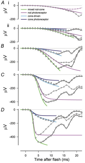
Stimulus energies increase from A to D. The data points show the recorded mixed rod–cone ERG (circles), the smaller cone-driven ERG obtained after suppressing the rods (triangles), and the isolated rod-driven ERG (squares). The purple and dark blue lines plot, respectively, the responses of models described in the text for the rod and cone photoreceptor responses; the light blue and the green lines show the model responses for the cone-driven ERG (cone photoreceptor response combined with a cone-driven postreceptoral component) and the mixed rod-cone ERG (modelled rod photoreceptor response combined with the modelled cone-driven ERG). At later times when the data points are not described by the models, they are joined by black lines (DE, sm469). A, blue flash: 23.5 sc. Td s, 7.1 ph. Td s. Ai and Aii show the responses to a blue flash that is in the linear range for the rods and rod-bipolar cells. Ai includes the response of the linear photoreceptor–rod-bipolar cell model (dashed purple line). The recorded response deviates from this combined model after about 12–13 ms due to intrusion of a negative postreceptoral component, but remarkably continues to follow the modelled rod photoreceptor response for several milliseconds. B, blue flash: 188 sc. Td s, 57 ph. Td s. C, white flash: 2300 sc. Td s, 1300 ph. Td s. D, white flash: 59 000 sc. Td s, 34 000 ph. Td s.

Although several observations indicate that the cone-driven a-wave includes an early negative postreceptoral component, it is not clear what cells or mechanisms generate this voltage. The results of PDA blockade are not definitive because PDA not only blocks the responses of OFF bipolar cells and horizontal cells, it also suppresses glutamatergic transmission in the more proximal retina. However, Bush & Sieving (1994) also showed that the photopic a-wave is essentially unaffected by APB, indicating that the negative postreceptoral component is not generated in the ON pathway, though this still leaves the possibility that the component is generated by proximal retinal cells of the OFF pathway rather than more directly by OFF bipolar cells themselves. We have found that NMDA produces some reduction in the amplitude of the cone-driven a-wave, indicating the presence of a contribution from postsynaptic responses of proximal retinal cells in addition to the contribution that probably arises from OFF bipolar cells (authors' unpublished observations).

Further indication of the origins of the postreceptoral component of the cone-driven a-wave are obtained by considering its time course. This component can be adequately modelled as the first integral of the cone photocurrent response (i.e. as the result of a process with a time constant of at least tens of milliseconds). If the ON pathway had been involved then it would have been more appropriate to assume a component generated as the third (or higher) integral of the cone signal, since the metabotropically activated ON bipolar cells will introduce additional integrations (Robson & Frishman 1995). In contrast, the ionotropic activation of OFF bipolar cells probably introduces little more than a very short delay, leaving a need only to explain the observed single integration. We may speculate that the component could be generated as a result of the response of Müller cells to a change in [K⁺]_o due to entry of K⁺ into OFF bipolar or more proximal cells at light onset and that it is the kinetics of the [K⁺]_o change that give rise to the integration. This idea is supported by our preliminary studies showing that the slow component can be removed by intravitreal injection of Ba²⁺ to block the effect on Müller cells of changes in [K⁺]_o by blocking the cells' K⁺ channels.

Rod and cone receptor models

A major emphasis of this work has been to provide improved descriptive mathematical models of the contributions of rod and cone photoreceptors to the flash-evoked ERG. To this end, for several interrelated reasons, we have modified the mathematical formulations that have previously been proposed.

Firstly we wished to provide models of the flash-evoked ERG that could in principle describe responses at times much later than the first few milliseconds during which the receptor components are the sole constituents of the response. Ideally, the models should describe the whole time course of the receptor response which, in the case of the rods, lasts hundreds of milliseconds and, in the macaque, peaks around 140 ms. For this reason, we have approximated the kinetics of the cascade with a low-pass filter having three independent stages. The assumption that the kinetics of the transduction cascade can be modelled as three simple first-order operations implies that inactivation of each of the active molecular species involved in the transduction cascade is a Poisson process so that the lifetimes of the active molecules are exponentially distributed Though it is believed that the inactivation of activated rhodopsin is not such a simple process (Rieke & Baylor, 1998; Whitlock & Lamb, 1999) but takes place in a number of stages so that the activity initially declines more slowly, this will have little effect on the early part of the overall response unless it is the lifetime of the activated rhodopsin that is the shortest of the three. We have relied upon probe-flash measurements of the later part of the derived rod-response waveform to estimate the values of the time constants involved. Although we are not very confident of the probe-flash measurements for the first half of the rising phase of this response, we found that estimates of the time constants were quite tightly constrained by the later, more reliable points. In all cases the tail of the recovery phase indicated a dominant time constant close to 150 ms while the relatively short time-to-peak (about 140 ms) could only be achieved if the shorter of the other two time constants was no more than about 30 ms. Secondly, we noted that for characterisation of the initial delay a transport delay was inappropriate if responses earlier than about twice the apparent delay time (2.5–3.5 ms) were considered. Therefore we could not expect to use this kind of delay to model the rising edge of any rod-driven a-wave whose amplitude comes close to saturation because, as seen in Fig. 13A, responses of this amplitude peak at 7 ms or less. Thus we adopted a form for the impulse response of the delay that was first suggested by Baylor et al. (1974). They indicated that a better fit to early responses of turtle cones could be obtained if they modified their six-stage filter model of the later time course of the responses by replacing the filter stage with the shortest time constant (10 ms) with a ten-stage filter in which each stage had a time constant one-tenth as long. As Baylor et al. (1974) pointed out, this ‘composite’ delay would provide a ‘fair representation of the delay introduced by diffusion of a small molecule over a distance of 2 or 3 μm’. Cobbs & Pugh (1987) adopted a four-stage version of this model to describe responses of salamander rods while Cideciyan & Jacobson (1996), who believed that the delay reflected the kinetics of three significant microsteps in the transduction cascade, modelled human rod a-waves using a composite delay with three stages.

As a generalisation of the idea of a composite delay we adopted the formulation given in eqn (2) or (3) which simply extends this idea to an n-stage delay where n is adjusted to provide the best fit of the model without prejudice as to the physical basis of the delay. For rod responses, the best fit was obtained with a delay having 12 or 13 stages, whereas a five-stage delay was best for cone responses. Although this difference in the form of the delay in rods and cones must relate to differences in the underlying physical processes and might reflect shorter diffusion distances in the cones, the nature of these differences cannot be determined from ERG measurements alone

Another useful modification to the rod and cone models was to reduce substantially the time constant of the ‘membrane filter’ that has been supposed to make the recorded ERG voltage change occur more slowly than the conductance change of the outer segment membrane that causes it. For rods we find that the time constant is not more than 0.2 ms - not very different from the value calculated by Penn & Hagins (1972) - while in cones it appears to be about 1 ms. These values are lower than previous estimates made from human ERG recordings of about 1 ms for rods (Smith & Lamb, 1997) and between about 2 and 5 ms for cones (Hood & Birch, 1993, 1995; Cideciyan & Jacobson, 1996; Smith & Lamb, 1997). For the rods our lower value is a consequence both of our adoption of a delay function that mimics the effect of an output filter on the very early part of the linear response and our assumption of a less abrupt saturation characteristic than exponential that mimics the effect of an output filter on the shape of the response to a very strong stimulus as it approaches the saturation level. This less abrupt saturation characteristic could be related to some non-uniformity in the intensity of the light reaching the retina or to some heterogeneity among the photoreceptors contributing to the response. With respect to the cones, the substantially shorter time constant for the ‘membrane filter’ is mainly a result of our identifying the slower part of the cone-driven a-wave as a postreceptoral ERG component rather than as a direct reflection of the cone photocurrent.

Parsing the dark-adapted ERG

Figure 14 summarises our empirical observations and the (modified) models that we have proposed for the leading edge of the a-wave of the macaque dark-adapted ERG. The figure shows that over a wide range of stimulus energies both rod- and cone-driven responses are influenced at early times by postreceptoral components in addition to the photocurrents of the receptors themselves. The cone-driven responses produce a substantial contribution to the dark-adapted ERG at all stimulus energies, and as previously described by Bush & Sieving (1994), the postreceptoral component can be larger than the receptoral component when stimulus energy is low. As energy is increased the receptoral component grows relative to the postreceptoral component, and at the highest energy in the figure provides about one-half of the cone-driven response. For a stimulus of this energy, the total cone-driven response contributes about one-fifth of the peak amplitude of the saturated a-wave, and rather more at later times.

For low stimulus energies that produce rod and rod-bipolar cell responses in the linear range at early times, the rod-driven negative-going postreceptoral components are also relatively large at the peak of the a-wave and play a major role in shaping this part of the waveform. This is illustrated in Fig. 14A in which the rod-driven ERG is shown together with the summed responses of linear models of the rod and rod-bipolar cell. Even though the combined response of rods and rod-bipolar cells starts to appear around 12–13 ms to peak at about 18 ms (see also Fig. 10), the contribution of the negative postreceptoral components to the rod-driven a-wave makes it follow fairly closely the time course of the rod receptor response for several milliseconds more than this, and to peak at a later time (e.g. Jamison et al. 2001). Thus, changes in the postreceptoral components in both rod and cone ERGs produced by adaptation, pharmacological manipulation or disease, may well result in changes in a-wave amplitude and peak time, particularly for responses in the linear range.

REFERENCES

- Baylor DA, Hodgkin AL, Lamb TD. The electrical responses of turtle cones to flashes and steps of light. J Physiol. 1974;242:685–727. doi: 10.1113/jphysiol.1974.sp010731. [DOI] [PMC free article] [PubMed] [Google Scholar]
- Baylor DA, Nunn BJ, Schnapf JL. The photocurrent, noise and spectral sensitivity of rods of the monkey Macaca fascicularis. J Physiol. 1984;357:575–607. doi: 10.1113/jphysiol.1984.sp015518. [DOI] [PMC free article] [PubMed] [Google Scholar]
- Breton ME, Schueller AW, Lamb TD, Pugh EN., Jr Analysis of ERG a-wave amplification and kinetics in terms of the G-protein cascade of phototransduction. Invest Ophthalmol Vis Sci. 1994;35:295–309. [PubMed] [Google Scholar]
- Bush RA, Sieving PA. A proximal retinal component in the primate photopic ERG a-wave. Invest Ophthalmol Vis Sci. 1994;35:635–645. [PubMed] [Google Scholar]
- Cideciyan AV, Jacobson SG. Negative electroretinograms in retinitis pigmentosa. Invest Ophthalmol Vis Sci. 1993;34:3253–3263. [PubMed] [Google Scholar]
- Cideciyan AV, Jacobson SG. An alternative phototransduction model for human rod and cone ERG a-waves: normal parameters and variation with age. Vision Res. 1996;36:2609–2621. doi: 10.1016/0042-6989(95)00327-4. [DOI] [PubMed] [Google Scholar]
- Cobbs WH, Pugh EN., Jr Kinetics and components of the flash photocurrent of isolated retinal rods of the larval salamander, Ambystoma tigrinum. J Physiol. 1987;394:529–772. doi: 10.1113/jphysiol.1987.sp016884. [DOI] [PMC free article] [PubMed] [Google Scholar]
- Dawson WW, Trick GL, Litzkow CA. Improved electrode for electroretinography. Invest Ophthalmol Vis Sci. 1979;18:988–991. [PubMed] [Google Scholar]
- Friedburg C, Thomas MM, Lamb TD. Time course of the flash response of dark- and light-adapted human rod photoreceptors derived from the electroretinogram. J Physiol. 2001;534:217–242. doi: 10.1111/j.1469-7793.2001.t01-1-00217.x. [DOI] [PMC free article] [PubMed] [Google Scholar]
- Hood DC, Birch DG. A quantitative measure of the electrical activity of human rod photoreceptors using electroretinography. Vis Neurosci. 1990a;5:379–387. doi: 10.1017/s0952523800000468. [DOI] [PubMed] [Google Scholar]
- Hood DC, Birch DG. The a-wave of the human electroretinogram and rod receptor function. Invest Ophthalmol Vis Sci. 1990b;31:2070–2081. [PubMed] [Google Scholar]
- Hood DC, Birch DG. Human cone receptor activity: the leading edge of the a-wave and models of receptor activity. Vis Neurosci. 1993;10:857–871. doi: 10.1017/s0952523800006076. [DOI] [PubMed] [Google Scholar]
- Hood DC, Birch DG. Phototransduction in human cones measured using the a-wave of the ERG. Vision Res. 1995;35:2801–2810. doi: 10.1016/0042-6989(95)00034-w. [DOI] [PubMed] [Google Scholar]
- Hood DC, Birch DG. Assessing abnormal rod photoreceptor activity with the a-wave of the electroretinogram: applications and methods. Doc Ophthalmol. 1997;92:253–267. doi: 10.1007/BF02584080. [DOI] [PubMed] [Google Scholar]
- Jamison JA, Bush RA, Lei B, Sieving PA. Characterization of the rod photoresponse isolated from the dark-adapted primate ERG. Vis Neurosci. 2001;18:445–455. doi: 10.1017/s0952523801183112. [DOI] [PubMed] [Google Scholar]
- Lamb TD, Pugh EN. A quantitative account of the activation steps involved in phototransduction in amphibian photoreceptors. J Physiol. 1992;449:719–758. doi: 10.1113/jphysiol.1992.sp019111. [DOI] [PMC free article] [PubMed] [Google Scholar]
- Murayama K, Sieving PA. Different rates of growth of monkey and human photopic a-, b- and d-waves suggest two sites of ERG light adaptation. Clin Vis Sci. 1992;7:385–392. [Google Scholar]
- Nusinowitz S, Hood DC, Birch DG. Rod transduction parameters from the a -wave of local receptor populations. J Opt Soc Am A. 1995;12:2259–2266. doi: 10.1364/josaa.12.002259. [DOI] [PubMed] [Google Scholar]
- Paupoo AAV, Mahroo OAR, Friedburg C, Lamb TD. Human cone photoreceptor responses measured by the electroretinogram a-wave during and after exposure to intense illumination. J Physiol. 2000;529:469–482. doi: 10.1111/j.1469-7793.2000.00469.x. [DOI] [PMC free article] [PubMed] [Google Scholar]
- Peachey NS, Alexander KR, Fishman GA, Derlacki DJ. Properties of the human cone system electroretinogram during light adaptation. Appl Opt. 1989;28:1145–1150. doi: 10.1364/AO.28.001145. [DOI] [PubMed] [Google Scholar]
- Penn RD, Hagins WA. Kinetics of the photocurrent of retinal rods. Biophys J. 1972;12:1073–1094. doi: 10.1016/S0006-3495(72)86145-9. [DOI] [PMC free article] [PubMed] [Google Scholar]
- Pepperberg DR, Birch DG, Hood DC. Photoresponses of human rods in vivo derived from paired-flash electroretinograms. Vis Neurosci. 1997;14:73–82. doi: 10.1017/s0952523800008774. [DOI] [PubMed] [Google Scholar]
- Press WH, Teukolsky SA, Vetterling WT, Flannery BP. Numerical Recipes in C. 2. Cambridge University Press; 1992. [Google Scholar]
- Pugh EN, Jr, Nikonov S, Lamb TD. Molecular mechanisms of vertebrate photoreceptor light adaptation. Curr Opin Neurobiol. 1999;9:410–418. doi: 10.1016/S0959-4388(99)80062-2. [DOI] [PubMed] [Google Scholar]
- Rieke F, Baylor DA. Origin of reproducibility in the responses of retinal rods to single photons. Biophys J. 1998;75:1836–1857. doi: 10.1016/S0006-3495(98)77625-8. [DOI] [PMC free article] [PubMed] [Google Scholar]
- Robson JG, Frishman LJ. Response linearity and kinetics of the cat retina: the bipolar-cell component of the dark-adapted electroretinogram. Vis Neurosci. 1995;12:837–850. doi: 10.1017/s0952523800009408. [DOI] [PubMed] [Google Scholar]
- Robson JG, Frishman LJ. Photoreceptor and bipolar-cell contributions to the cat electroretinogram: a kinetic model for the early part of the flash response. J Opt Soc Am A. 1996;13:613–622. doi: 10.1364/josaa.13.000613. [DOI] [PubMed] [Google Scholar]
- Robson JG, Frishman LJ. Dissecting the dark-adapted electroretinogram. Doc Ophthalmol. 1999;95:187–215. doi: 10.1023/a:1001891904176. [DOI] [PubMed] [Google Scholar]
- Robson JG, Saszik SM, Frishman LJ. Receptoral and post-receptoral components of the a-wave of the primate dark-adapted electroretinogram (ERG) ARVO Abstracts. 2002 (1821) [Google Scholar]
- Robson JG, Viswanathan S, Frishman LJ, Ahmed J. Derived rod response and contributions of rod and off-pathway signals to the macaque electroretinogram a-wave. Invest Ophthalmol Vis Sci Suppl. 1999;40:S15. [PubMed] [Google Scholar]
- Schnapf JL, Nunn BJ, Meister M, Baylor DA. Visual transduction in cones of the monkey Macaca fascicularis. J Physiol. 1990;427:681–713. doi: 10.1113/jphysiol.1990.sp018193. [DOI] [PMC free article] [PubMed] [Google Scholar]
- Sieving PA, Murayama K, Naarendorp F. Push-pull model of the primate photopic electroretinogram: a role for hyperpolarizing neurons in shaping the b-wave. Vis Neurosci. 1994;11:519–532. doi: 10.1017/s0952523800002431. [DOI] [PubMed] [Google Scholar]
- Slaughter MM, Miller RF. 2-Amino-4-phosphonobutyric acid: a new pharmacological tool for retina research. Science. 1981;211:182–185. doi: 10.1126/science.6255566. [DOI] [PubMed] [Google Scholar]
- Smith NP, Lamb TD. The a-wave of the human electroretinogram recorded with a minimally invasive technique. Vision Res. 1997;37:2943–2952. doi: 10.1016/s0042-6989(97)00094-1. [DOI] [PubMed] [Google Scholar]
- Thomas MM, Lamb TD. Light adaptation and dark adaptation of human rod photoreceptors measured from the a-wave of the electroretinogram. J Physiol. 1999;518:479–496. doi: 10.1111/j.1469-7793.1999.0479p.x. [DOI] [PMC free article] [PubMed] [Google Scholar]
- Whitlock GG, Lamb TD. Variability in the time course of single photon responses from toad rods: termination of rhodopsin's activity. Neuron. 1999;23:337–351. doi: 10.1016/s0896-6273(00)80784-9. [DOI] [PubMed] [Google Scholar]