Properties of the human muscle nicotinic receptor, and of the slow-channel myasthenic syndrome mutant εL221F, inferred from maximum likelihood fits

Abstract

The mechanisms that underlie activation of nicotinic receptors are investigated using human recombinant receptors, both wild type and receptors that contain the slow channel myasthenic syndrome mutation, εL221F. The method uses the program HJCFIT, which fits the rate constants in a specified mechanism directly to a sequence of observed open and shut times by maximising the likelihood of the sequence with exact correction for missed events. A mechanism with two different binding sites was used. The rate constants that apply to the diliganded receptor (opening, shutting and total dissociation rates) were estimated robustly, being insensitive to the exact assumptions made during fitting, as expected from simulation studies. They are sufficient to predict the main physiological properties of the receptors. The εL221F mutation causes an approximately 4-fold reduction in dissociation rate from diliganded receptors, and a smaller increase in opening rate and mean open time. These are sufficient to explain the approximately 6-fold slowing of decay of miniature synaptic currents seen in patients. The distinction between the two binding sites was less robust, the estimates of rate constants being dependent to some extent on assumptions, e.g. whether an extra short-lived shut state was included or whether the EC₅₀ was constrained. The results suggest that the two binding sites differ by roughly 10-fold in the affinity of the shut receptor for ACh in the wild type, and that in the εL221F mutation the lower affinity is increased so the sites become more similar.

The discovery of the genetic basis for many of the human congenital myasthenic syndromes (Engel et al. 1999; Beeson & Newsom-Davis, 2000) has added to the inherent interest in investigation of the relationship between structure and function in the nicotinic acetylcholine receptor (AChR) of the muscle endplate. The slow channel congenital myasthenic syndromes result from single amino acid ‘gain-of-function’ mutations in the receptor protein that give rise to prolonged endplate currents. Muscle weakness is thought to result from endplate damage caused by excess calcium entry. In addition, at physiological rates of stimulation the prolonged endplate potentials summate, leading to persistent depolarisation at the endplate and the consequent inactivation of the voltage-gated sodium channels.

From the point of view of protein structure-function relations, it is important to know how a mutation changes the receptor function in order to produce slower decay of synaptic currents (see Unwin et al. 2002; Colquhoun et al. 2003b). It has recently been shown, both theoretically and experimentally, that the time constants for the decay of synaptic currents should be the same as the time constants for the distribution of the burst length of the underlying single ion channels (Colquhoun et al. 1997; Wyllie et al. 1998). This is true, at least, if the burst length is measured at zero concentration (after a pulse of agonist), or at sufficiently low concentrations in the steady state. The term burst length here refers to an experimental estimate of the length of an individual activation of the ion channel, i.e. the visible part of what happens between the time when the agonist first associates with the receptor and the time when it finally dissociates from the receptor. The term activation is defined more precisely by Edmonds et al. (1995), Wyllie et al. (1998) and Béhéet al. (1999). For most channels an average activation consists of several openings, not just one.

There are two extreme ways in which a mutated channel could produce longer activations, and therefore slower decay of synaptic currents. On one hand, the number of channel openings during each activation might be similar for wild type and mutant, but each opening is on average in the mutant, longer so the activation is longer. This would happen if the mutation slowed down the shutting rate of the open channel, an effect on the conformation change involved in gating. At the other extreme, the individual openings in the mutant might have exactly the same mean duration as for the wild type (or even be shorter), but there would be more of them - the activation would look much like that for the wild type but go on for longer. This would, for example, be expected if the mutation caused the acetylcholine to dissociate more slowly from the resting (shut) state of the receptor, an effect on the binding reaction. The longer occupancy of the shut state would give more time for the channel to re-open, before dissociation prevented it from doing so. However a similar outcome would be seen if the mutation had a quite different effect, to speed up the rate of the opening conformational change (a gating effect), which would also favour re-opening of the channel. To understand how the protein works it is essential to disentangle these effects, i.e. to solve the binding-gating problem. This problem, and its close relationship to the classical pharmacological problem of separating affinity and efficacy, has been reviewed by Colquhoun (1998).

It was proposed (Colquhoun & Hawkes, 1977; Colquhoun & Sakmann, 1981, 1985) that the binding-gating problem could be solved by analysis of the fine structure of channel activations. In that work, distributions of shut times, open times, burst lengths etc. were fitted, and interpreted retrospectively in terms of the rate constants in a proposed reaction scheme. Since then, more subtle methods for analysis of the problem have been developed. Horn & Lange (1983) proposed that the rate constants should be fitted directly to the (idealised) data by choosing them so as to maximise the likelihood of the whole sequence of open and shut times. But for this method to be useful in practice it is essential to know the distributions of the apparent open and shut times that are actually observed, i.e. to allow properly for missed brief openings and shuttings. It has been developed, by two groups, into a method that can be used routinely, with publicly available programs. Qin et al. (1996) used an approximate missed events correction (the QUB programs), while Colquhoun et al. (1996) used the exact solution to the missed events problem given by Hawkes et al. (1990) and Hawkes et al. (1992), on the basis of which the HJCFIT program used in this paper was developed. Methods for correction for missed events, and the background for maximum likelihood fitting, are discussed at greater length in the accompanying paper Colquhoun et al. (2003a).

The advantages of direct maximum likelihood fitting include the following. (a) The whole of the information in the record is extracted in one operation (including information about correlations between events that tells us about connections between states), (b) the underlying rate constants in the mechanism are estimated directly, rather than inferred from separate fits to several different sorts of distribution, and (c) the simultaneous fitting of several records at different concentrations with a single set of rate constants is straightforward.

The HJCFIT method is used here to analyse a mutation in the ε subunit of the human nicotinic receptor, εL221F, that has been found to underlie a typical slow channel myasthenic syndrome (Oosterhuis et al. 1987; Croxen et al. 2002). Despite the fact that this amino acid is in, or close to, the first transmembrane, M1 region, rather than in the extracellular N-terminal region, and is in the ε subunit rather than the α subunit, the effect of the mutation appears to be predominantly, though not exclusively, to increase the affinity of acetylcholine for the resting state of the receptor.

METHODS

Source of DNAs

cDNAs encoding the human muscle AChR α, β, δ and ε subunits (Beeson et al. 1993) were subcloned into the mammalian expression vector pcDNA3.1 (Invitrogen).

The εL221F missense mutation was introduced into the ε subunit using the Sculptor in vitro mutagenesis system kit (Amersham Pharmacia, UK) using the oligonucleotide primer 5′-GAAGCCGTTCTTCTACGTCATTAACAT-3′, which contains the mutant εC661T nucleotide transition. Restriction endonuclease digestion with Ear I and DNA sequence analysis were used to check for the presence of the mutation and to ensure no additional DNA changes had been introduced. The nicotinic receptor subunits were co-transfected with pTracer (Invitrogen) which contains cDNA encoding green fluorescent protein.

Cell culture

Human embryonic kidney (HEK 293) cells were maintained in continuous culture at 37 °C, 5% CO₂ in Dulbecco's modified Eagle's medium containing 10% fetal calf serum and 1% penicillin/streptomycin. Cells were transfected transiently using standard calcium phosphate techniques. Briefly, cells were plated onto poly-d-lysine-coated glass coverslips 4–6 h before transfection (such that cells were 30–40% confluent) in 4-well tissue culture dishes containing 0.5 ml of standard medium. Each cDNA (1–2 μg μl⁻¹) was added to 55 μl of ice-cold CaCl₂ (340 mm), which was then added dropwise to 75 μl of Hepes-buffered saline containing (mm): 280 NaCl, 2.8 Na₂HPO₄, 50 Hepes (pH adjusted to 7.2 with NaOH) and allowed to stand at room temperature for 20 min. This produced the fine suspension of calcium phosphate crystals required for high efficiency transfection. A 30 μl portion of this suspension was then added to each well, giving a total of 2.75 μg of cDNA in the ratio 2:1:1:1:6, α:β:δ:ε:GFP, or α:β:δ:εL221F:GFP, for wild type and mutant respectively. The medium was changed after 14–16 h and electrophysiological experiments were started 18–40 h after transfection.

Electrophysiological methods and solutions

Cell-attached recordings

Steady state single channel recordings of recombinant human nicotinic acetylcholine (ACh) channel activity in cell-attached patches were made at −100 mV with an extracellular solution containing (mm): 5.4 NaCl, 142 KCl, 1.8 CaCl₂, 1.7 MgCl₂ and 10 Hepes (pH adjusted to 7.4 with KOH). Patch-pipettes were made from thick-walled borosilicate glass (Clark Electromedical, Reading, UK) and filled with extracellular solution containing ACh (1 nm−30 μm). After fire-polishing their tips, pipettes had resistances of 8–15 MΩ. Single-channel currents were recorded with an Axopatch 200A amplifier (Axon Instruments, California, USA), filtered at 10 kHz and stored on digital audio tape (DAT) for subsequent analysis (Biologic DTR 1204, Biologic Instruments, Claix, France).

Outside-out patch recording

Steady state single channel recordings from outside-out patches were used to assess the reduction in apparent single channel conductance caused by channel block by high concentrations of ACh. An extracellular recording solution of composition (mm): 150 NaCl, 2 KCl, 1.8 CaCl₂, 1.8 MgCl₂ and 10 Hepes (pH adjusted to 7.4 with NaOH) was employed. Patch-pipettes were filled with an ‘internal’ recording solution that contained (mm): 2.5 NaCl, 110 KCl, 10 EGTA and 10 Hepes (pH adjusted to 7.4 with KOH). For outside-out patch recordings ACh (30 μm−10 mm) was applied in the bath and single-channel currents for measurement of equilibrium channel block, for which only apparent amplitudes were required, were filtered at 0.5–1 kHz and stored on DAT tape for subsequent analysis. Data were played back from DAT tape and digitised continuously at 5–10 kHz. The apparent amplitudes of events were fitted using the SCAN program as for cell-attached patches (see below). After fitting, stability plots were inspected using the EKDIST program and for stable experiments, apparent amplitudes were fitted after imposition of a suitable resolution (usually 50–200 μs).

Whole-cell patch recordings

These were made in essentially the same manner as outside-out patch recordings with the following exceptions. Patch-pipettes were made from thin-walled borosilicate glass (Clark Electromedical, Reading, UK). After fire-polishing whole-cell pipettes had resistances of 2–5 MΩ. Whole-cell concentration-response curves were constructed on lifted HEK 293 cells, using focal application of ACh (100 nm−200 μm) via a gravity-fed automated 30-way solenoid valve system (built in-house), connected to a SF-77B Perfusion fast-step (Warner Instruments Corp., Hamden, CT, USA) stepper motor and 3-barrel pan pipe. Solutions had to be degassed to avoid bubble formation. Using this system, the time to peak response was approximately 10–20 ms, so quite short pulses of agonist (100 ms) could be applied. Tests showed that a 15 s interval between agonist pulses was sufficient for recovery. Lines were flushed with test solution for 2 s before stepping from control to test solution. Whole-cell currents were recorded on DAT, filtered at 0.5 kHz. Data were played back from DAT tape on to an oscilloscope and peak current recorded for construction of concentration- response curves, which were fitted by weighted least squares (with the program CVFIT).

Analysis of data from cell-attached patches

Single-channel currents from cell-attached patches were replayed from DAT tape. Data from cell-attached patches were filtered at 8 kHz and digitised continuously at 80 kHz. The amplitudes and durations of events were fitted by time-course fitting using the SCAN program (see Colquhoun & Sigworth, 1995). On average 17 500 transitions were fitted per patch.

After fitting, the EKDIST program was used to inspect stability plots, and, for stable experiments, to fit distributions of amplitudes, shut times, open period duration and various burst properties, in the usual way (Colquhoun & Sigworth, 1995). An apparent open period is defined as a period when the channel appears to be continuously open (regardless of amplitude); often it will be extended by missed brief shuttings. A resolution of 20–30 μs was imposed on the data before fitting distributions.

Bursts of openings were defined as groups of openings, each group being separated by apparent shut times longer than a specified duration, t_crit. The aim is to define bursts such that it is very likely that all openings in a burst originate from the same individual channel; this is all that matters for HJCFIT (it is not essential for activations to be well separated, except insofar as this is a way to be sure that all openings are from one channel). In practice, at low concentrations of ACh (up to 1 μm) the burst has to be defined so that it corresponds, as closely as possible, to a single activation of the channel, as defined above. At higher concentrations (10 μm and greater), bursts can be defined as the much longer clusters of activations that are separated by long silent periods when all the channels in the patch are desensitised (Sakmann et al. 1980; Colquhoun & Ogden, 1988).

Estimation of rate constants with HJCFIT

The distributions of durations were fitted (in EKDIST) with mixtures of arbitrary numbers of exponential probability density functions. For the purposes of understanding mechanism it is not these arbitrary time constants that are needed, but the rate constants in the postulated receptor reaction scheme, these being (insofar as a realistic mechanism can be postulated) the quantities that have a real physical significance. This was achieved by calculating, from the postulated mechanism, the likelihood of the entire sequence of apparent open and shut times, in the order in which they occur. The order matters, because open and shut times are correlated (Colquhoun & Sakmann, 1985), so the probability of seeing an open time of say 2.1 ms depends on the length of the preceding shut time. The calculation of the likelihood has to use conditional distributions that take this into account. There are many brief events (especially brief shuttings) that are too short to be resolved, so the open time distributions given by, for example, Colquhoun & Hawkes (1982), which assume perfect resolution, cannot be used. Instead we have to use distributions that describe the apparent open and shut times that we actually observe. Several approximate solutions to this problem have been proposed (see, for example, Colquhoun & Hawkes, 1995, and the accompanying paper, Colquhoun et al. 2003a). However there is no need for approximations as an exact solution to the problem was found by Hawkes and Jalali (Hawkes et al. 1990, 1992; Jalali & Hawkes, 1992a, b; Colquhoun et al. 1996). This exact solution is used by the program HJCFIT to calculate the likelihood of the entire sequence of apparent open and shut times, and to adjust the values of the rate constants in the mechanism so as to maximise this likelihood. This method, and its use to fit simulated data, was illustrated by Colquhoun et al. (1996) where full details of the method can be found (see also Colquhoun & Hawkes, 1995; Colquhoun et al. 2003a, and the HJCFIT program manual).

At low ACh concentrations (up to 1 μm here) the longest section of record that can be ‘guaranteed’ to originate from one channel consists of the individual channel activations, each consisting of a few channel openings in quick succession. A critical shut time, t_crit, was used to define bursts of openings so that each burst represents, as accurately as possible, an individual activation. When more than one channel is present, the interval between one activation and the next (for a single channel) may be longer than that observed, but it must be at least t_crit, and this knowledge is used in the calculation of the likelihood for each burst by using the initial and final vectors defined by Colquhoun, Hawkes & Srodzinski (1996, eqns (5.8), (5.11)), and these will be denoted CHS vectors. Simulations show that their use is important when fitting short bursts in low concentration records (Colquhoun et al. 2003a).

At high agonist concentrations (10–30 μm here), a slightly different procedure is used. Under these conditions, long clusters of activations occur, with a sufficiently high probability of being open that one can be sure that all the openings in a cluster originate from one channel (Sakmann et al. 1980; Colquhoun & Ogden, 1988). These clusters are separated by very long shut times, that were presumed to represent periods during which all the channels in the patch were desensitised. In this case the likelihood of the whole cluster is calculated on the assumption that it originates from one channel. It is still necessary to divide the record into bursts (clusters in this case) by use of a suitable t_crit, but in this case the CHS vectors were not used to start and end the likelihood calculation for each cluster because the mechanisms being fitted did not contain the desensitised states (the steady state vectors were used instead). Because the clusters are quite long, the effect of the method of calculation of initial and final vectors is, in any case, much smaller than for short bursts at low concentrations. This procedure, which does not need any detailed knowledge of desensitisation mechanisms, can be justified by simulations (Colquhoun et al. 2003a).

At the end of each fit, a numerical estimate of the Hessian matrix was made, to allow printing of the approximate standard deviations of the estimates, and the matrix of correlation coefficients between pairs of estimates (see Colquhoun et al. 2003a, for more details). These provided a useful guide to the reliability of the estimates, but all the errors given in Tables 1–4 were not found in this way, but from the variability that was observed when the experiment was repeated several times.

Table 1.

Separate patches: means of the estimates of rate constants for wild type receptors (scheme 1, with sites assumed to be independent)

		Fixed rate fits (n = 18)		EC50 constrained fits (n = 12)
α2	s−1	2290	± 9%	2460	± 16%
β2	s−1	53 200	± 8%	51600	± 11%
α1a	s−1	4860	± 16%	6000	± 20%
β1a	s−1	450	± 45%	37.7	± 45%
α1b	s−1	89700	± 25%	71300	± 25%
β1b	s−1	224	± 25%	156	± 62%
k−1a=k−2a	s−1	3510	± 25%	1330	± 39%
k+1a=k+2a	m−1 s−1	2.2 × 108*	—	2.23 × 107†	± 38%
k−1b=k−2b	s−1	12500	± 14%	13400	± 15%
k+1b=k+2b	m−1 s−1	5.05 × 108	± 22 %	4.70 × 108	± 29%
k−2a+k−2b	s−1	16000	± 11%	14700	± 13%
β2/(k−2a+k−2b)	—	3.32	± 13%	3.52	± 16%
E2	—	23.3	± 4%	21.0	± 8%
Ka≡K1a=K2a	μm	15.9	±25%	59.7	±54%
Kb≡K1b=K2b	μm	24.8	± 25%	2.84	± 31%
EC50	μm	3.67	± 23%	16.8*	± 0%

Each estimate was as obtained by HJCFIT analysis (with mechanism 1 as in Fig. 6A) of a single patch, at a range of ACh concentrations (30 nm–100 μm). In order to allow all the rate constants to be estimated without knowing the number of channels in low concentration patches, either one of the association rate constants was fixed (left column), or one of the rate constants was constrained to produce the specified EC₅₀ (right column). The ten rate constants are shown in the first ten rows, followed by various quantities derived from them. The total dissociation rate from diliganded receptors, k_−2a+k_−2b, is referred to in the text. The ratio β₂/(k_−2a+k_−2b) gives the number of re-openings per activation for diliganded receptors in isolation. E₂=β₂/α₂, is the efficacy, or gating constant, for diliganded receptors. The binding equilibrium constants for the a and b sites are denoted K_a and K_b. Because of the assumption that the sites are independent, K_a=K_1a=K_2a, where, for example, K_1a=k_−1a/k_+1a. Mean rate constants are given with errors expressed as the coefficient of variation of the mean (as a percentage), i.e. mean ± 100 ×c.v.m.

^*Fixed rate constants

^†rate constants constrained by EC₅₀. Microscopic reversibility was used to determine k_+1a.

Table 4.

Simultaneous fit of several patches: means of the estimates of rate constants for _εL221 F receptors (scheme 2, with sites assumed to be independent)

		Free fits (n = 3 sets)		EC50 constrained fits (n = 4 sets)		Fits with 4 rates fixed to wild-type values (n = 5 sets)
α2	s−1	1440	± 7%	1440	± 8%	1390	± 8%
β2	s−1	86 300	± 3%	85 000	± 4%	82 000	± 7%
α1a	s−1	3200	± 15%	3110	± 9%	3510	± 9%
β1a	s−1	43.5	± 35%	12.2	± 59%	9.09	± 60%
α1b	s−1	57 100	± 10%	57 000	± 10%	61 200	± 4%
β1b	s−1	114	± 44%	14.6	± 81%	8.27	± 70%
k−1a=k−2a	s−1	1750	± 35%	409	± 26%	363	± 46%
k+1a=k+2a	m−1 s−1	5.16 × 108	± 49%	1.74 × 107	± 67%	6.81 × 106	± 43%
k−1b=k−2b	s−1	1950	± 61%	3210	± 16%	3430*	—
k+1b=k+2b	m−1 s−1	6.95 × 108	± 43 %	3.69 × 108	± 51 %	2.33 × 108*	—
αD	s−1	6500	± 17%	9400	± 41%	5020	± 33%
βD	s−1	12.2	± 7%	19.3	± 37%	13.3	± 37%
k−2a+k−2b	s−1	3700	± 20%	3300	± 13%	3790	± 4%
β2/(k−2a+k−2b)	—	23.3	± 20%	25.8	± 17%	21.6	± 8%
E2	—	59.9	± 5%	59.0	± 5%	58.8	± 7%
ED	—	0.002	± 18%	0.002	± 18%	0.003	± 15%
Ka≡K1a=K2a	μm	3.39	± 60%	23.5	± 72%	53.3	± 63%
Kb=K1b=K2b	μm	2.81	± 74%	8.72	± 53%	14.7*	—
EC50	μm	0.75	± 64%	4.14*	—	4.14*	—

Left, free fit often rate constants. Centre, same except the EC50 was constrained to be 4.14 μm. Right, free fit of 5 rate constants, the rate constants for association and dissociation from the b site(^*)being fixed at the values found for wild type (see Table 3), and the EC₅₀ fixed at 4.14 μm.

After fitting to obtain values for the rate constants, the ability of the fit to describe the experimental results must be tested. The quality of the fit can be judged by the standard deviations of the rate constants, and the correlations between them (Colquhoun et al. 2003a), but mainly the tests are graphical. The observations are displayed as histograms (or mean open times) and the appropriate HJC distribution is calculated from the fitted rate constants (together with the known resolution) and the curve so predicted is superimposed on the data to see how well it fits (e.g. Figs 7, 8, 11 and 12). As well as showing the fit to apparent open and shut times, the extent to which the fit can account for correlations can be tested too. A histogram can be constructed to show the observed conditional distribution of apparent open times, by including only those openings that are adjacent to apparent shut times in a specified range. The predicted conditional distribution can be calculated as described by Colquhoun et al. (1996) and superimposed on the histogram to see how well it fits (e.g. Fig. 11 and Fig. 12). A more synoptic view of correlations can be obtained from a ‘conditional mean open time plot’. To construct this, a set of shut time ranges is defined, and the mean apparent open time is found for openings that are adjacent to shut times in each range. This mean open time is plotted against the mean of all shut times in each range. The plot of observations constructed in this way can then be compared with the HJC values calculated from the fitted rate constants (and known resolution) as described by Colquhoun et al. (1996). For examples, see Figs 10, 11, 12 and Colquhoun et al. (2003a).

Figure 7. Direct estimation of rate constants from individual patches, assuming independent binding sites (fixed forward rate).

A, wild type apparent open time and shut time distributions from channel activity evoked by 30 nm, 100 nm and 30 μm ACh (left to right). The solid line in each case shows the predicted HJC distribution for each patch, calculated from the fitted rate constants and resolution, and superimposed on the histogram of experimental observations. The dashed lines show the predicted ideal distributions with perfect resolution. B, apparent open and shut time distributions as in A but for the εL221F receptor recorded in the presence of 30 nm, 50 nm and 10 μm ACh (left to right).

Figure 8. Direct estimation of rate constants from individual patches, assuming independent binding sites (forward rate constrained by EC₅₀).

A, wild type apparent open time and shut time distributions for the same three patches as shown in Fig. 7A. The solid lines are the HJC distributions calculated from the fitted rate constants for each patch superimposed on the histogram of experimental observations; the dashed lines show the predicted ideal distributions. B, as A but for the same three εL221F patches shown in Fig. 7B.

Figure 11. Direct estimation of rate constants from multiple patches, scheme 1 assuming independent binding sites.

A, results of simultaneous fitting of rate constants to three wild type patches (50 nm, 100 nm and 10 μm ACh respectively, left to right), association rates were neither fixed nor constrained by the EC₅₀. Top row, apparent open times, second row, apparent shut times. The solid lines in each case show the predicted HJC distribution calculated (for the appropriate ACh concentration) from the single set of estimated rate constants found by fitting all three patches simultaneously. The dashed lines show the predicted ideal distributions. Third row, conditional HJC distributions (solid lines) of apparent open times adjacent to shut times in the range t < 0.1 ms superimposed on the experimentally observed open times adjacent to shut times in the same range. The dashed lines show the HJC distributions of all apparent open times. Bottom row, conditional mean apparent open time plots (see Methods and text). The diamonds with error bars (joined by solid lines) show the experimental data. The solid circles show the HJC predictions for the same shut time ranges that were used for the data and the dashed line shows the continuous relationship between mean open time and adjacent shut time calculated from the fitted rate constants. The arrows indicate the t_crit for each patch: experimentally observed shut times greater than this value may be underestimated because we do not know the number of channels in the patch and they are shown for illustrative purposes only. B, as A but shows the results of simultaneous fitting of rate constants to three εL221F patches (100 nm, 1 μm and 10 μm ACh respectively, left to right).

Figure 12. Direct estimation of rate constants from multiple patches, scheme 2 assuming independent binding sites (constrained by EC₅₀).

A, results of simultaneous fitting of rate constants to the same three wild type patches shown in Fig. 11A (50 nm, 100 nm and 10 μm ACh respectively, left to right), unconstrained estimations of forward rates with scheme 2 resulted in unrealistically fast forward rates, consequently one of the forward rates in the fits shown was constrained by the EC₅₀. Top row, apparent open times, second row, apparent shut times. The solid lines in each case show the predicted HJC distribution calculated from the estimation of rate constants from all three patches simultaneously, superimposed on the histogram of experimentally observed events for each patch in turn. The dashed lines show the predicted ideal distributions. Third row, conditional HJC distributions (solid lines) of apparent open times adjacent to shut times in the range t < 0.1 ms superimposed on the experimentally observed open times adjacent to shut times in the same range. The dashed lines show the HJC distributions of all apparent open times. Bottom row, conditional distributions of mean open time adjacent to specified shut time ranges plotted against apparent shut time. The solid lines show the observed correlation from experimental data, the dashed lines show the predicted correlation calculated from the rate constants by HJCFIT. The arrow indicates the t_crit for each patch, experimentally observed shut times greater than this value will be underestimated as we do not know the number of channels in the patch and they are shown for illustrative purposes only. B, as A but shows the results of simultaneous fitting of rate constants to the same three εL221F patches shown in Fig. 11B (100 nm, 1 μm and 10 μm ACh respectively, left to right), again with one of the forward rates constrained by the EC₅₀ as for wild type data. C, as B but shows the results of fitting the same three εL221F patches with the binding and unbinding rates for the b site fixed to the mean wild type values, the remaining forward rates were constrained by the EC₅₀.

Figure 10. Effect of adding an extra shut state on direct estimation of rate constants from individual patches (fixed forward rate).

A, direct estimation of rate constants from a wild type patch in the presence of 100 μm ACh with either scheme 1 (top) or scheme 2 (extra shut state added, below). As before, HJC distributions of apparent open and shut times (solid lines) are shown superimposed on the histograms of experimental observations, dashed lines show the predicted ideal distributions calculated from the fitted rate constants (left and centre panels). The right hand column shows the conditional mean apparent open time plotted against adjacent shut time, as described in Methods and text. The diamonds with error bars (joined by solid lines) show the experimental data. The solid circles show the HJC predictions for the same shut time ranges that were used for the data, and the dashed line shows the continuous relationship between mean open time and adjacent shut time calculated from the rate constants fitted for scheme 1 (top right) or scheme 2 (lower right). B, as A but showing the results of direct estimation of rate constants from an εL221F patch exposed to 30 μm ACh, with either scheme 1 (upper panels) or scheme 2 (bottom panels).

Unless otherwise stated, means are given together with the standard deviation of the mean (s.d.m., also known as the standard error), or with the coefficient of variation of the mean (c.v.m.) expressed as a percentage of the mean.

The HJCFIT program, and all other programs used here, can be obtained from http://www.ucl.ac.uk/Pharmacology/dc.html.

RESULTS

Equilibrium concentration-response curves

Figure 1 shows the response to ACh measured by fast application to whole cells (see Methods). The time to peak response was about 10 to 20 ms. This may not be quite fast enough to avoid totally the effects of desensitisation, the fastest component of which has a time constant of about 50 ms in mouse muscle (Franke et al. 1993).

Figure 1. Whole-cell responses to acetylcholine of HEK 293 cells transiently expressing human wild type and εL221F neuromuscular junction nicotinic acetylcholine receptors.

A, typical whole-cell current responses recorded from lifted HEK 293 cells at −100 mV. Wild type (WT) human neuromuscular junction nicotinic ACh receptors produced large inward currents in response to focal application of ACh with a maximum around 200 μm. εL221F nicotinic receptors were more sensitive to ACh, reaching a maximum at around 50 μm. Vertical scale bar 5 nA, horizontal scale bar 100 ms. B, averaged log concentration-response curves for wild type (solid line, n = 5 cells) and εL221F (dashed line, n = 5 cells) nicotinic receptors. Responses were normalised with respect to their fitted maximum and are shown fitted with the Hill equation, constrained to be parallel and with a maximum fixed at 1. Error bars show s.d.m.

The curves shown are based on 21 curves from five cells for wild type receptors, with ACh concentrations from 0.1 to 200 μm, the number of responses being from 17 to 21 at each concentration apart from the lowest. The curves for the εL221F receptor were based on 20 curves from five cells with concentrations from 0.2 to 200 μm. Each curve was fitted with either a Hill equation, or with a mechanism like scheme 1 (Fig. 6, but lacking singly liganded openings); the EC₅₀ values were very similar for either fit. The curves were then normalised to the maximum found in each fit. The curves were sufficiently similar that the normalised responses at each concentration were averaged, and these are shown in Fig. 1. Separate fits of the Hill equation to each curve gave EC₅₀ values of 13.6 μm for wild type and 4.14 μm for εL221F. The curves were essentially parallel (n_H= 1.40 and 1.44 respectively). In Fig. 1, the Hill curves have been constrained to be parallel, and the relative potency of ACh on the two receptors is estimated to be 3.23 ± 0.13.

Figure 6. Kinetic schemes used for direct estimation of rate constants.

A, scheme 1, binding of the agonist (A) to two non-equivalent binding sites, denoted a and b. Open states are denoted by ^*. Opening rate constants are denoted β_x, shutting rate constants as α_x, association rate constants as k_+x and dissociation rate constants as k_−x. The subscripts 1, 2 refer to the order (1st, 2nd) of binding. B, scheme 2, as scheme 1 except that an extra shut state is added to the right of the diliganded open state. Because transition into this extra ‘desensitised’ state does not involve binding, the rate constant into it is denoted β_D and the rate constant for leaving it is denoted α_D. C, simplified version of scheme 1, showing examples of the three types of activation seen in cell-attached patch recordings. Each class of activation is shown next to the open and shut states from which, we suggest, it arises.

Apparent open period and shut time distributions

It is immediately obvious when looking at single channel currents recorded in HEK 293 cells expressing either human α₂βδε (wild type) or α₂βδεL221F (εL221F) receptors (Fig. 2) that individual activations of εL221F receptors are prolonged compared with wild type.

Figure 2. Steady state activations of wild type and εL221F nicotinic receptor channels activated by acetylcholine.

A, continuous 1 s recordings of wild type (upper trace) and εL221F (lower trace) channel activity evoked by nanomolar concentrations of ACh. Activations of εL221F receptors are on average longer then activations of the wild type receptor. B, continuous 10 s recordings of wild type (upper trace) and εL221F (lower trace) channel activity evoked by micromolar concentrations of ACh. At these higher concentrations, channel activity occurs in clusters often lasting a second or more, separated by long silent periods (desensitised gaps). Note also that these silent periods are sometimes interrupted by brief channel openings. All records are shown filtered at 6.25 kHz.

After generating an idealised list of apparent open and shut times in SCAN, apparent open periods were fitted with between 1 and 3 exponential components and apparent shut times with mixtures of 4 to 6 exponential probability density functions in EKDIST. For wild type patches, apparent open periods for low concentration experiments, 30–100 nm (Fig. 3, see also Fig. 4) were best fitted by a mixture of three exponential components (solid lines in Fig. 3). Attempts to fit with only two components (dashed lines in Fig. 3) were consistently unsatisfactory.

Figure 3. Open period distributions from wild type nicotinic channels fit with mixtures of two or three exponential probability density functions.

Examples of open period distributions of wild type nicotinic channels at low ACh concentration, showing best fits with mixtures of two (dashed line) or three (solid line) exponential probability density functions (pdfs).

Figure 4. Open period and shut time distributions for wild type and εL221F channels.

A, distributions of the apparent open period and shut time lengths for wild type nicotinic receptor channels. Open periods were fitted with a mixture of three exponential probability density functions (pdfs) at low ACh concentrations (30 nm and 100 nm), tending towards two (at 10 μm) or one (at 30 μm) exponential pdf at higher concentrations. Shut time distributions were fitted with mixtures of 4 to 6 exponential pdfs. B, apparent open period and shut time distributions for εL221F nicotinic receptor channels. In contrast to wild type channels, open periods for εL221F channels were always fitted best by a mixture of 3 exponential pdfs, and shut times with mixtures of 4–6 pdfs.

The observation of three, rather than two, components suggests that the receptor has (at least) three open states, and their concentration dependence suggests that two of them are monoliganded. Thus it seems that there are two different monoliganded states, as might be expected if the two binding sites are not identical. Figure 4 shows the results of fits to four wild type (panel A) and four εL221F (panel B) patches over a range of ACh concentrations. At higher concentrations, 10 and 30 μm (Fig. 4A) apparent open periods could be fitted with two and one exponential components respectively. The values of the time constants (τ) for the exponentials were not obviously dependent on ACh concentration, being approximately 25 μs (τ₁), 400 μs (τ₂), and 1.2 ms (τ₃). At the lowest concentration, 30 nm, τ₁ accounted for 23%, τ₂ 67% and τ₃ 10% of apparent open periods. As agonist concentration increased the areas of the fastest two time constants, τ₁ and τ₂ decreased, whilst the area attributable to the longest time constant τ₃ increased. At 100 nm, the area of τ₁ had decreased to 13%, τ₂ was the most affected, now accounting for only 27% of apparent open periods, whilst τ₃ increased to 60%. By 10 μm, apparent open periods could be fitted adequately with two exponential components, the area attributable to τ₂ having decreased to zero, the shortest component of apparent open periods distributions, τ₁ still accounted for 7% of apparent open periods, whilst 93% was now of the longest 1.2 ms type (τ₃). By 30 μm, essentially 100% of observed open periods were of the longest type (τ₃) and the open period distribution was fitted adequately with only one exponential probability density function.

The situation was somewhat different for apparent open period distributions from εL221F patches (compare top rows in Fig. 4A and Fig. 4B). Throughout the concentration range tested, 10 nm to 30 μm, apparent open period distributions for the mutant receptor were best fitted by a mixture of three exponential probability density functions. The fastest component of the open period distributions, τ₁ was of approximately the same duration as for wild type at around 20 μs, the second component was more variable in length than with wild type, but was on average of similar duration at around 400 μs, the longest component, τ₃ was however, noticeably longer than for wild type at around 4.5 ms.

The fastest component, τ₁ of the open period distributions did decrease in relative area with increasing agonist concentration as in the wild type, but unlike the wild type, it did not disappear altogether at the highest concentrations tested. The fast time constant, τ₁ accounted for around 30% of apparent open periods at low (10–100 nm) agonist concentration, but only around 10% at higher (10–30 μm) ACh concentration. Conversely, τ₃, the longest component of the apparent open period distribution increased in area with increasing agonist concentration, accounting for around 55% of observed open periods at low agonist concentrations and increasing to around 75% at high agonist concentrations. The intermediate component, τ₂, remained virtually unaffected, accounting for around 10% of apparent open periods across the range of agonist concentrations tested.

Apparent shut time distributions (see lower rows of histograms in both Fig. 4A and B) were superficially similar for wild type and εL221F receptors. The predicted shortest component has a time constant, τ₁, that is about 13 μs for both. This is below the resolution set in these experiments (25 μs), but these very short shuttings are frequent so there are quite enough above 25 μs to fit, and their relative (extrapolated) area is 70–90% of all shut times. A second slightly longer component, τ₂, of between 30 and 100 μs accounts for around 1–3% of the relative area. These first two components are consistent across the whole range of concentrations tested and therefore most probably represent shuttings that occur within an activation. The third component of the shut time distributions, τ₃, has a duration of around 1 ms at low ACh concentration (30 or 100 nm for wild type, 10 to 100 nm for εL221F receptors), but increases to around 3 ms at higher ACh concentrations (10 or 30 μm for both wild type and εL221F receptors). The relative area of τ₃ is also concentration-dependent, accounting for only a fraction of a percentage of apparent shut times at low ACh concentrations, but increasing to between 10 and 20% of apparent shut times for the wild type receptor, and to around 5% for the εL221F-containing receptor, at higher ACh concentrations. This is similar to the small ‘intermediate’ shut time component detected in frog muscle receptors by Colquhoun & Sakmann (1985). It is this component which gives rise to the hump seen clearly in the shut time distributions for both wild type (Fig. 4A) and εL221F (Fig. 4B). Its presence at low concentrations shows that these ‘1 ms’ shut times occur within individual activations of the channel, so the critical shut time, t_crit, used to define bursts of openings (that are intended to define individual activations) was set between this component and the longest shut time component (see Methods). The longest components of the apparent shut time distributions were fitted with between one and three exponential components. This component of shut times decreased in relative area as ACh concentration increased for both wild type and εL221F receptors. At high concentrations, very long shut times appeared that were presumed to represent periods during which all the channels in the patch were desensitised (Sakmann et al. 1980; Colquhoun & Ogden, 1988).

The length of the shut times between activations (bursts) will generally be an underestimate of their true length for a single channel. This is because we have no way of knowing how many channels we have in our patch and therefore, no way of knowing whether the open periods which flank these long shut times arise from the same receptor or from different receptors.

Apparent burst length

The most important quantity from the physiological point of view, is the length of channel activations (low concentration burst length), because this is what will determine the decay rate of synaptic currents (Wyllie et al. 1998). The length of bursts, at least for those that arise from diliganded receptors, is also relatively immune to errors that arise from missed brief events.

By means of a suitable t_crit (see Methods, and above) we can separate the idealised single channel record created in SCAN into bursts which, to a good approximation, each represent an individual activation. Figure 5 shows examples of burst length distributions for wild type and εL221F receptors in the presence of 100 nm ACh. In each case, the burst length distribution can be fitted with a mixture of four exponential probability density functions.

Figure 5. Burst length distributions for wild type and εL221F channels.

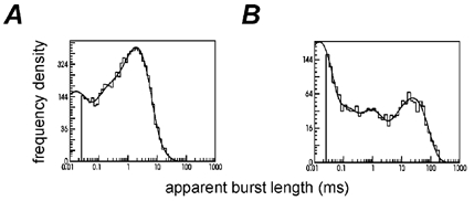
A, example of the burst length distribution for wild type channels (100 nm ACh), fitted with a mixture of 4 exponentials with means (and areas) of 13 μs (20%), 140 μs (13%), 1.8 ms (63%) and 4.1 ms (4%). Overall mean burst length was 1.3 ms. B, example of the burst length distribution for εL221F channels (100 nm ACh), again fitted with a mixture of 4 exponentials with mean (and areas) of 14 μs (61%), 84 μs (10%), 763 μs (11%) and 23.8 ms (18%). Overall mean burst length was 4.6 ms.

The time constants of the first two components are remarkably similar for both wild type and εL221F receptors, although their areas differ somewhat. The shortest component, τ₁, was of around 13 μs in either case, but accounted for 20% of wild type and 60% of εL221F bursts. τ₂ was around 100 μs and accounted for about 10–15% of observed bursts in either type of receptor. τ₃ was in this case longer for wild type (1.8 ms, 60% of area) than for εL221F receptors (1 ms, 11%), but was on average similar. However, the longest component of the burst length distribution, τ₄, was on average much longer and of greater area for εL221F receptors (24 ms, 20%) than wild type (4 ms, 5%). This longest component of the burst length distribution is the most important for physiological purposes as it carries the majority of the charge in the steady state record, and because there should be a similar long time constant in the macroscopic response to a short pulse of agonist (Wyllie et al. 1998), and hence in the synaptic current. It is shown later (Fig. 13) that the calculated pulse response is close to having single exponential decay with a time constant that is very similar to the longest component of the burst length distribution.

Figure 13. Simulated synaptic currents.

The curves show the current evoked by a 0.2 ms pulse of 1 mm ACh (the pulse is marked as an upward deflection in the line at the top). The calculations (done in the program SCALCS) used the rate constants from Table 3 (right column) for the wild type, and from Table 4 (middle column) for the εL221F receptor. The dashed line shows the predicted response for wild type receptors, and the solid line shows the predicted response of εL221F receptors.

The effect of this long component is, in this example, to make the overall mean burst length for the εL221F receptor 3.5-fold longer (4.6 ms) than for the wild type (1.3 ms).

Choice of mechanism

It is essential that the mechanism should describe physical reality if physical conclusions are to be drawn. It seems desirable, therefore, that a postulated mechanism should be based on what is known about structure (see, for example, Unwin et al. 2002; Colquhoun et al. 2003b). Since it is known that there are two binding sites, and that their environments differ, a good starting point is the mechanism shown in Fig. 6 (scheme 1), which was suggested by Colquhoun & Sakmann (1985), and has often been used since (e.g. Milone et al. 1997).

This reaction scheme contains four simplifications (see also the Discussion and Colquhoun et al. 2003a).

1. It does not include states that open with no ligand, because we see none and so cannot fit them.

2. It does not contain desensitised states, because it is not our aim here to investigate desensitisation.

3. It does not include channel block by agonist, because we operate in a range where block is negligible, and have shown that inclusion of block makes no difference.

4. It postulates that the three open states do not intercommunicate directly. Although direct transitions from one to another probably occur they are likely to be infrequent and to have little effect on our conclusions (Grosman & Auerbach, 2001).

The fact that the open states are not connected allows us to consider three different sorts of channel activation. Examples of roughly what each looks like are shown on the diagrammatic representation of the mechanism in Fig. 6C.

Scheme 2 (Fig. 6) is the same as scheme 1 apart from addition of an extra shut state. This extra short-lived state was introduced by Salamone et al. (1999) to describe the observation of more shut times with an apparent lifetime of about 1 ms than was predicted by scheme 1 in work with the adult nicotinic ACh receptor. They found that the rate of entry into, and exit from, the extra shut state were not dependent on agonist concentration. The physical significance of the extra state is quite obscure. It could be regarded as a very short-lived desensitised state (desensitisation is known to take place on a wide range of time scales, Elenes & Auerbach, 2002).

This scheme, in which the two binding sites (denoted the a and b sites) differ, was found to describe adequately most features of the activity of both wild type and εL221F. Most of the estimates of rate constants from individual patches were made with the customary assumption that the two binding sites were independent (see Discussion). In other words, we assume that binding of a molecule of ACh to the a site does not affect binding of a second molecule of ACh to the b site and vice-versa. Using the rate constants defined in Fig. 6, this means imposing the following three constraints during fitting.

(1)

The additional constraint of microscopic reversibility assures that also:

(2)

The number of free rate constants to be estimated is thus reduced from 14 to 10. Because we do not know how many channels are present in the patch at low ACh concentrations, all recordings at concentrations less than 1 μm were fitted in bursts, so apparent shut times longer than t_crit (usually 2 to 5 ms) were excluded, and the CHS start and end vectors were used (see Methods and Colquhoun et al. 2003a). With this fitting procedure there is no information about the absolute frequency of channel activations (unless a high concentration is fitted simultaneously). To provide this missing information, something else must be supplied and this can be done, either by specifying arbitrarily one of the rate constants, or, better, by using the measured EC₅₀ to calculate one rate constant from the values of all the others. Either procedure reduces to nine the number of rate constants to be estimated.

In view of the fact that three exponentials rather than two are needed to fit open period durations at low concentrations, it is not surprising that attempts to fit rate constants with HJCFIT using reaction schemes with only one or two open states were found to describe the observations adequately only in a subset of experiments.

It will be convenient in describing the results to distinguish between those rate constants that refer only to the fully occupied (diliganded) receptor, and those rate constants that require a distinction between the two binding sites to be made. The former group, the ‘diliganded parameters’, consist of the rate constants for the opening (β₂) and shutting (α₂) of the diliganded receptor, and the total rate of dissociation of agonist from it, (k_−2a+k_−2b). These are the values that can be estimated most robustly, and also the values that are of the greatest physiological relevance (Colquhoun et al. 2003a). All the other rate constants are rather harder to estimate accurately, and of less relevance to the shape of synaptic currents. Nevertheless, in order to understand the protein properly it is very desirable to know how the two binding sites differ from each other.

Direct estimation of rate constants from individual patches with a fixed forward rate constant, and the assumption that the two binding sites are independent

In the first fits, k_+1a was fixed to an arbitrary, but physically plausible value, 2.2 × 10⁸m⁻¹ s⁻¹. This value could, of course, be wrong, in which case the estimates of some other parameters will be wrong too. In particular, the estimate of β_1b might be poor, though the diliganded parameters should be little affected (Colquhoun et al. 2003a).

Figure 7 shows examples of the results of estimation of rate constants in this way.

In each graph, the histogram shows the observed data, while the solid line shows the theoretical HJC distribution superimposed on the histogram. Notice particularly that the solid line is not fitted to the histogram in any case. Rather it is calculated from the estimates of the rate constants that have already been found by HJCFIT, with allowance for missed events. It will fit the histogram of observations only insofar as the mechanism used in HJCFIT, and the estimates of the rate constants for it, are adequate to describe the observations. The histograms are not used for fitting, but as a visual test of the adequacy of the maximum likelihood fitting that is completed before histograms are drawn (see also Methods). The dashed lines in Fig. 7 show the ideal distribution calculated from the fitted parameters with no allowance for missed events (using the simpler methods of Colquhoun & Hawkes, 1982). The discrepancy between solid and dashed lines is therefore an indication of the extent to which open and shut times have been distorted by the omission of short shut and open times (those below the resolution).

For both wild type (Fig. 7A) and εL221F (Fig. 7B), patches over a range of concentrations (30 nm to 100 μm for wild type, 1 nm to 30 μm for εL221F), rate constants estimated with scheme 1 could predict quite well the observed open and shut period distributions. Fits of this sort were done separately on 18 patches at a range of ACh concentrations. The means of the 18 sets of rate constant estimates so obtained are shown in Table 1 (left column) for wild type, and in Table 2 (left column) for εL221F.

Table 2.

Separate patches: means of the estimates of rate constants for _εL221 F receptors (scheme 1, with sites assumed to be independent)

		Fixed rate fits (n = 9)		EC50 constrained fits (n = 5)
α2	s−1	1180	± 9%	1060	± 14%
β2	s−1	72 000	± 4%	70600	± 7%
α1a	s−1	10 000	± 41%	10 500	± 45%
β1a	s−1	404	± 77%	104	± 50%
α1b	s−1	156 000	± 60%	100 000	± 32%
β1b	s−1	304	± 20%	3.96	± 34%
k−1a=k−2a	s−1	956	± 29%	985	± 34%
k+1a=k+2a	m−1 s−1	2.20 × 108*	—	4.62 × 106†	± 35%
k−1b=k−2b	s−1	3050	± 20%	3050	± 38%
k+1b=k+2b	m−1 s−1	7.61 × 108	± 18%	9.31 × 108	± 7%
k−2a+k−2b	s−1	4000	± 18%	4030	± 33%
β2/(k−2a+k−2b)	—	18	± 17%	17.5	± 34%
E2	—	61	± 6%	66.7	± 9%
Ka≡K1a=K2a	μm	4.02	± 26%	213	± 49%
Kb≡K1b=K2b	μm	4.01	± 27%	3.27	± 38%
EC50	μm	0.93	± 36%	4.62*	± 35%

Mean rate constants and corresponding equilibrium constants, exactly as in Table 1, but for mutant receptor. Each value was found by fitting a separate patch (ACh concentration, 1 nm to 10 μm).

The ‘diliganded rate constants’ were well defined with, on average, β₂, the diliganded opening rate constant being about 50% faster in εL221F receptors than in wild type, while α₂, the diliganded shutting rate was halved. The combined effect of these results in a 3-fold increase in E₂=β₂/α₂, the efficacy of gating for diliganded openings for the mutant receptor. The biggest effect, however, was on total dissociation rate (k_−2a+k_−2b) from the diliganded shut state, A₂R, which was decreased 4-fold in the mutant compared with wild type. The scatter was greater for the estimates of rate constants that required the two binding sites to be distinguished from one another. One sort of monoliganded opening, that which occurs when only the b site is occupied, appears to be very brief, and barely resolvable (1/α_1b= 11.1 μs) whereas the other is easily resolvable (1/α_1a= 206 μs). The opening rate constants for both types of monoliganded openings are low, but not very precisely defined. The rate of dissociation of ACh from the a site, which has been assumed to be the same whether or not the b site is occupied (k_−2a=k_−1a), seems to be a good deal slower than dissociation from the b site, though the equilibrium affinities for the two sorts of site are similar. Note, however, that the equilibrium constants in Table 1 are calculated from the mean rate constants in the upper part of the table, with an error derived from them by Fieller's theorem (e.g. Colquhoun, 1971). The scatter of the values is such that substantially different values for the affinities are found if the equilibrium constants are calculated separately for each of the 18 experiments, and then averaged. When calculated in this way, K_a= 15.9 μm± 25% (the same as in Table 1), but K_b= 122 μm± 43% (compared with 24.8 μm± 25% in Table 1). This discrepancy is simply a result of scatter and illustrates the margin of uncertainty in the results.

Estimation of rate constants from individual fits with forward rate constrained by EC₅₀

Rather than fixing the value of a rate constant to an arbitrary value, it is preferable to use a known EC₅₀ value to provide the information that is missing when no assumption is made about the number of channels in the patch (Colquhoun et al. 2003a). Therefore HJCFIT estimation was repeated on individual patches, but with the value of k_+1a=k_+2a calculated at each iteration from the EC₅₀ value obtained from whole-cell concentration- response curves (see Fig. 1). The fits to a given experiment were slightly less good when done this way, as judged by the maximum likelihood that was achieved (no doubt because the fits without EC₅₀ constraint gave, on average, a somewhat lower EC₅₀ than was found in the whole cell experiments). The decreased quality of the fit was not ‘statistically significant’ as judged by a likelihood ratio test in 2/7 experiments with wild type, and in 3/5 experiments with mutant receptors, though on average the reduction in the maximum log-likelihood produced by imposition of the EC₅₀ constraint was 16 units for wild type and 11 units for mutant. Nevertheless the decrease in quality of fit was small by eye and it was still possible in most cases to obtain tolerably good predictions of the observed open and shut time distributions after correction for missed events. Examples of HJC distributions obtained in this way are shown in Fig. 8 for the same three wild type and the same three εL221F patches as were shown in Fig. 7. Note for example the slight discrepancy between the HJC distribution predicted by the fitted rate constants and the observed data for short open periods in high ACh concentration patches (upper rightmost histograms in Fig. 8A and B for wild type and εL221F respectively).

The mean rate constants obtained in this way are shown in the right hand columns of Table 1 (wild type) and Table 2 (εL221F). Diliganded rate constants were little different from those obtained from the fixed rate estimations. For example, α₂ for wild type was around 2500 s⁻¹vs. 2300 s⁻¹ for the fixed rate fit (1100 s⁻¹vs. 1300 s⁻¹ for εL221F). β₂, E₂ and total dissociation from A₂R (k_−2a+k_−2b) were similarly unaffected by the use of the EC₅₀ constraint. This is exactly as expected on the basis of the robustness of the estimates of diliganded rate constants found by Colquhoun et al. (2003a). Among the other rate constants, the estimates of association and dissociation for binding to the b site did not differ greatly between the two methods of estimation, and neither did α_1a and α_1b. Agreement was less good for β_1a and β_1b. The major difference lay in the association rate constant for the a site, k_+1a=k_+2a, which was the rate constant constrained by the EC₅₀. For the wild type receptor, this was estimated to be 2.2 × 10⁷m⁻¹ s⁻¹, about 10-fold slower than the fixed value used for the first estimation. For the εL221F receptor it was 4.6 × 10⁶m⁻¹ s⁻¹, about 50-fold slower. For wild type receptors, the dissociation rate constant for the a site, k_−1a=k_−2a, was also slower when estimated with the EC₅₀ constraint, by about 3-fold, but the estimates were similar by both methods for εL221F.

Channel block by ACh at high agonist concentration

Figure 9A shows the decrease in apparent current amplitude of single-channel receptor currents recorded in the outside-out patch configuration.

Figure 9. Block of wild type nicotinic receptors by high concentrations of ACh.

A, typical channel activity recorded at −100 mV in an outside-out patch from a HEK 293 cell expressing the human wild type neuromuscular junction nicotinic ACh receptors exposed to high concentrations (0.03–10 mm) of ACh. The apparent amplitude of single-channel activations decreases as ACh concentration increases. All records are shown filtered at 1 kHz. Horizontal scale bar 0.5 s, vertical scale bar 2 pA. B, plot of apparent single channel amplitude against log concentration, fitted with the Hill equation. Points show mean (±s.d.m.) from 11 patches, n_H (±s.d.m.) = 0.986 ± 0.025; IC₅₀ (±c.v.m.) = 1.56 mm± 5.9%.

The currents were heavily filtered (0.5–1 kHz) to obtain average amplitudes. As ACh concentration was increased from 30 μm to 10 mm, the apparent amplitude decreased. This was interpreted as being caused by rapid blockages of the channel by ACh (see Colquhoun & Sakmann, 1985; Ogden & Colquhoun, 1985; Sine & Steinbach, 1987). In this case the fractional reduction of mean amplitude represents the proportion of time for which the open channel is blocked by ACh. Figure 9B shows the apparent amplitude as a function of ACh concentration, for the wild type receptor. The points are means from 11 patches, fitted with the Hill equation. At −100 mV the IC₅₀ was 1.56 mm± 5.9% (mean ±c.v.m.) and the Hill slope was 0.986 ± 0.025 (mean ±s.d.m.). Since the Hill slope was almost exactly 1, the IC₅₀ can be interpreted as the equilibrium constant (at −100 mV) for block of the open channel by ACh.

Note that little channel block (less than 6%) was seen at concentrations below 100 μm. It is, therefore, not surprising that inclusion of channel block in the mechanism (scheme 1) used for estimation of rate constants did not significantly affect the estimation of the doubly liganded rate constants, α₂, β₂ or total dissociation rate from the doubly liganded receptor, nor did it improve the quality of the fit even at the highest concentrations tested (100 μm for wild type and 30 μm for εL221F receptors, data not shown).

Including an additional short-lived shut state in the reaction scheme

Fits with and without this extra state are compared, for both wild type and εL221F, in Fig. 10.

Fits are shown for the highest agonist concentration used in this study (100 μm for wild type and 30 μm for εL221F). Inclusion of an additional short-lived shut state (Fig. 6, scheme 2), did not substantially improve the quality of the HJC distribution predictions of the observed open periods and shut times, nor did it have a significant effect on the conditional open time distribution (compare upper and lower rows of histograms in Fig. 10A and B). Estimates of the ‘diliganded rates’ were similar with or without the extra shut state, and separate fits with the extra state, using either an arbitrarily fixed association rate constant, or an EC₅₀-constrained rate constant, gave somewhat different binding rates, but the results were qualitatively similar to those in Table 1 (right) and Table 3; they suggested that the affinity of the b site was rather higher than for the a site. In the case of the εL221F receptor, addition of the extra shut state made even less difference to the rate constant estimates than for wild type. However there is some doubt whether the extra shut state that was fitted here, to human receptors, is the same phenomenon as that observed by Salamone et al. (1999) in mouse receptors. Their extra state had a mean lifetime of around 1 ms whereas the fits here all gave longer lifetimes (about 14 ms for wild type and 53 ms for εL221F receptors).

Table 3.

Simultaneous fit of several patches: means of the estimates of rate constants for wild type receptors (scheme 2, with extra shut state)

		Free rate fits (n = 4 sets)		EC50-constrained fits (n = 4 sets)
α2	s−1	1840	± 10%	1860	± 11%
β2	s−1	52 000	± 4%	52000	± 4%
α1a	s−1	6550	± 17%	7660	± 38%
β1a	s−1	414	± 99%	369	± 98%
α1b	s−1	78 200	± 31%	80 200	± 43%
β1b	s−1	3.75	± 33%	3.90	± 59%
k−1a=k−2a	s−1	11 200	± 4%	10 400	± 4%
k+1a=k+2a	m−1 s−1	9.04 × 107	± 26%	6.69 × 107	± 24%
k−1b=k−2b	s−1	2150	± 52%	3430	± 41%
k+1b=k+2b	m−1 s−1	1.49 × 108	± 30 %	2.33 × 108	± 5 %
αD	s−1	689	± 51%	777	± 39%
βD	s−1	65.3	± 33%	49.3	± 27%
k−2a+k−2b	s−1	13 300	± 8%	13 800	± 9%
β2/(k−2a+k−2b)	—	3.92	± 9%	3.74	± 20%
E2	—	28.4	± 7%	27.9	± 7%
ED	—	0.09	± 26 %	0.07	± 19 %
Ka≡K1a=K2a	μm	123	± 27%	155	± 25%
Kb≡K1b=K2b	μm	14.4	± 60 %	14.7	± 41 %
EC50	μm	9.32	± 21%	11.3*	± 21%

Sites were assumed to be independent. Four sets of patches, each set with three or more concentrations of ACh, were fitted and the result from each set was averaged. For results in the left column the EC₅₀ constraint was not used; for the fits on the right column the EC50 was fixed at 11.3 μm^*.

Simultaneous fits to multiple patches with scheme 1 assuming independent binding sites

In principle, the optimum method for estimation is a simultaneous fit of a single set of rate constants to several recordings made at different ACh concentrations. This method makes use of more sorts of information than fitting of a single record, and allows a direct test of the ability of the mechanism, and a single set of rate constants, to describe the behaviour of the channel over a range of concentrations. Furthermore, when the number of channels is unknown, simultaneous fitting precludes the necessity to fix a rate constant or to specify an EC₅₀, as shown by simulations (Colquhoun et al. 2003a). While very desirable in principle, simultaneous fitting will work well only if the patches that are pooled are indeed described by a single set of rate constants, i.e. if all channels are the same. In practice, recombinant channels in different patches often seem to vary in their characteristics by more than would be expected by chance (see Discussion). Patches for simultaneous analysis were selected to have similar apparent open time distributions.

Rate constants were estimated by simultaneous fit of a single set of rate constants to several records at different ACh concentrations (2–5 different patches for wild type and 2–3 for εL221F). Initially it was assumed that the two binding sites are independent (i.e. the constraints in eqns (1) and (2) were applied). Examples of three-patch fits obtained in this way with scheme 1 are shown for wild type (Fig. 11A, 50 nm, 100 nm and 10 μm) and εL221F (Fig. 11B, 100 nm, 1 μm and 10 μm) receptors. Both sets contained a high concentration that had long bursts of activations all from one channel (see Methods), so in this case it was not necessary to fix one rate constant, nor to constrain one with the macroscopic EC₅₀. Simulations show that simultaneous fits of recordings at a low and high concentration can provide reasonable estimates of all 10 free parameters when the binding sites are independent (Colquhoun et al. 2003a).

Wild type receptors

For wild type receptors, the HJC distributions of open periods predict well the observed data for these three patches (see top row of histograms in Fig. 11A). Predictions of apparent shut time distributions, however, were less accurate. Only shut times shorter than t_crit can be predicted. i.e. shorter than 2 ms, 3.5 ms and 35 ms (left to right, for 50 nm ACh, 100 nm and 10 μm respectively). At the lowest concentration, 50 nm, there are clearly more of the ‘intermediate’ (approximately 1 ms) shut times than are predicted by the fitted rate constants. At the highest concentration the longest (‘between activation’) shut time component is predicted to be somewhat shorter than was observed (see second row of histograms in Fig. 11A).

Open periods adjacent to short shuttings (shut time between the resolution, 25 μs, and 100 μs) were predicted well at all concentrations (see third row of histograms in Fig. 11A).

The bottom row of graphs in Fig. 11A shows the conditional mean apparent open time plot (see Methods and Fig. 10 and Fig. 12). The solid line shows the observations (the error bars are quite large in some ranges, because few shut times are observed in these ranges). The points (circles) show the HJC values calculated from the fitted rate constants (the dashed line is the theoretical continuous HJC relationship between open and adjacent shut times). At low concentrations, the mean falls with increasing adjacent shut time as expected for the negative correlation between observed open and shut times, and this fall is observed to occur mostly over shut times up to 0.1 ms or 0.2 ms. There was reasonable general agreement between observation and prediction, apart from the unexpected decline at long shut times at 10 μm. This unpredicted decline results largely from the existence of some very brief openings during the long shut periods during which all channels are supposed to be desensitised. Some of these are visible in Fig. 2B; their origin is unknown. They do not occur to any noticeable extent in oocytes or native channels, and there are not enough of them to prevent the apparent open time distribution at high concentration being fitted well by a single exponential distribution (see Figs 4A, 7A, 8A, 10A and 11A). But there are enough of them to show in the conditional mean open time plot. Note also that shut times longer that t_crit, 35 ms in this case, will be underestimated if there is more than one channel in the patch so the points at longer times (where the decline is seen) should really be some unknown distance to the right of where they are plotted.

εL221F receptors

A simultaneous fit of scheme 1 to three concentrations, assuming independence of the sites, is shown in Fig. 11B. The fits to shut times and conditional open times (rows 2 and 3) are quite good, but the fit to open periods of εL221F receptors is not so good. The most serious discrepancy is the existence of a modest number of short openings (top right graph) even at the highest concentration (10 μm), that is not predicted by any of the mechanisms that we have tested. These openings again are predominantly the brief openings that are seen, unexpectedly, during the long shut times that result from desensitisation (some can be seen in Fig. 2B). It is these unexpected openings that also cause the unpredicted fall in mean open time for openings adjacent to the longest shut times (bottom right graph). This phenomenon is similar to that seen in wild type receptors, though the brief openings are somewhat longer and/or more numerous in the mutant receptor so they are more obvious in the distribution of all open times at 10 μm.

Simultaneous fits to multiple patches with scheme 2 assuming independent binding sites

Inclusion of an extra shut state (scheme 2) was tested by simultaneous fit of the same sets of three wild type and three εL221F patches, with the results shown in Figs 12A and B, again assuming independence of the two binding reactions.

Initially no rate constants were either fixed or constrained by the EC₅₀. In the case of the wild type receptor, the fit to shut times was clearly improved by inclusion of the extra shut state (compare second row of histograms in Fig. 11A and Fig. 12A). However the prediction of the plot of conditional mean apparent open time against adjacent shut time tended to be rather worse than when the extra shut state was omitted (compare Fig. 11A and Fig. 12A, bottom left). The main fall in mean open time in the data always occurred at very short shut times, being almost complete after 0.1 ms, whereas the rate constants fitted in Fig. 12A predict that the fall will not occur until adjacent shut times exceed 10 ms, a discrepancy of 100-fold (see Discussion).

The εL221F receptor was fitted quite well with the extra shut state present (Fig. 12B), apart from the existence of unpredicted short openings at the highest ACh concentration, as described above. However the fits were also quite good without the extra shut state (Fig. 11B), so the extra shut state is not necessary.

Three to five sets of recordings of the sort illustrated in Fig. 11 and Fig. 12 were fitted, and the average results are given in Table 3 (wild type) and Table 4 (εL221F).

Mean rate constants obtained without fixing the EC₅₀ are shown in Table 3 (left column) for wild type and Table 4 (left column) for εL221F. The predicted EC₅₀ for wild type was about right, but for the εL221F receptor it was rather low, and also the estimates of the association rates (5 × 10⁸m⁻¹ s⁻¹ and 7 × 10⁸m⁻¹ s⁻¹ for the a and b sites respectively) were verging on being implausibly fast. Consequently the fits were repeated including the EC₅₀ as an additional constraint on an association rate constant for both wild type and εL221F receptors.

Mean rate constants obtained from EC₅₀-constrained simultaneous fits with scheme 2 are shown in Table 3 (right hand column), for wild type (4 runs from 15 patches) and Table 4 (middle column), for εL221F (5 runs from 12 patches). The values for the rate constants of the diliganded parameters, α₂, β₂ (and for E₂ the efficacy of diliganded openings) and total dissociation from the diliganded shut state A₂R are in good agreement with the values obtained with scheme 1 and from estimates from individual patches (Tables 1 and 2).

As before, there is less certainty about the rate constants that require the two sites to be distinguished from one another.

Wild type

The shutting rates for monoliganded openings when the a site only is occupied, α_1a, is consistently 5000–7000 s⁻¹, corresponding to a mean open time of 0.12–0.2 ms (compared with about 0.5 ms for the diliganded channel). When only the b site is occupied, the openings are very short indeed and barely resolvable, α_1b being over 70 000 s⁻¹. The opening rates for both sorts of monoliganded openings are not very consistent, but are certainly small, especially for the b site. The association and dissociation rate constants show reasonable consistency for those fits that predict something like the right EC₅₀ (i.e. excluding Table 1, left column). They imply that the affinity of ACh for the b site is roughly 10 times greater than for the a site, because of both faster association and slower dissociation. The values will be summarised in the Discussion.

εL221F receptors

The mean lifetimes of singly liganded open states are rather longer for the simultaneous fits than for separate fits, about 0.3 ms when the a site only is occupied, and again very brief (1–17 μs) when only the b site is occupied. The estimates of association and dissociation rate constants are generally similar for separate and simultaneous fits, but both predict rather low EC₅₀ values when this is not fixed. The effect of fixing the EC₅₀ to its observed value is largely to reduce the estimate of k_+1a, the value of which is therefore somewhat uncertain. Nevertheless the results in Tables 2 and 4 suggest that the affinities for the two sites are more similar than for the wild type.

The rate constants for the extra shut states in the wild type (Table 3) give a mean lifetime for this state of about 1.4 ms. An ‘opening’ spends less than 10% of the time in the extra shut state (E_D=β_D/α_D [ww2] 0.08). These values are similar to those found by Salamone et al. (1999). For the εL221F receptor the time spent in the extra shut state is very small (E_D= 0.02) which confirms the impression that the extra state is not necessary to describe the mutant receptor.

Simultaneous fits to multiple patches with scheme 1 without assuming independence of the two binding sites

The fit to intermediate shut times was improved by postulation of an extra short-lived shut state. The existence of this extra state in scheme 2 (Fig. 6) is essentially an empirical manoeuvre to fit the observations, but it is not known what the physical meaning of such a state might be. It is possible to get an equally good fit without having to postulate extra states in scheme 1 by abandoning the assumption that binding to the two sites is independent.

This approach predicted the open periods, shut times and conditional open period distributions with similar accuracy to the fit (Fig. 12A) with an extra shut state. In these fits the predicted conditional mean open time plot (for low concentrations) fell rapidly at short shut times, as observed, but was predicted to rise somewhat again at longer times. No such rise could be detected in the observations, though it must be remembered that shut times longer than t_crit long shut times cannot be measured properly. The results of the fits suggest, for the wild type, that binding to either the a site or to the b site was reduced (largely because of faster dissociation) if a molecule was already bound to the other site. However, this approach was not pursued further because simulations (Colquhoun et al. 2003a) show that it is not possible to obtain good estimates of all 13 rate constants unless it can be assumed that the low concentration records originate from one channel only, and we cannot do this.

Fits to the mutant receptor with one site constrained to be the same as wild type

Comparison of the simultaneous fits to wild type and mutant receptors suggests that binding to the a site may be much more affected by the mutation than binding to the b site. For example with the EC₅₀ fixed, k_+1b=k_+2b= 2.33 × 10⁸m⁻¹ s⁻¹ for wild type (Table 3) and 3.69 × 10⁸m⁻¹ s⁻¹ for εL221F (Table 4), and k_−1b=k_−2b= 3430 s⁻¹ for wild type and 3210 s⁻¹ for εL221F. Since the mutation is in the ε subunit it might well affect only one of the two (interfacial) binding sites, so the simultaneous fits on the εL221F receptor were repeated with the association and dissociation rate constants for the b site fixed at the values found for wild type.

Figure 12C shows an example of the quality of the fits for one three-patch set. HJC distributions calculated from the fitted rate constants are superimposed on the experimentally determined histograms for the same set that was shown in Fig. 12B. The HJC distributions obtained in this way show a slightly poorer prediction of the experimental data than the free fits, but are still tolerably good for all observations. Mean rate constants from five runs (12 patches) are shown in Table 4 (right hand column). The rate constants so found do not differ greatly from the comparable fit (Table 4, centre column) in which this was not done (apart perhaps from a further reduction in the estimate of k_+1a).

Simulation of synaptic currents from the fitted rate constants

The mechanism, and the rate constants that are fitted, should be able to predict the shape of any type of macroscopic current. Figure 13 shows the time course of miniature endplate currents, simulated as the response to a 0.2 ms pulse of 1 mm ACh. The calculations (done in the program SCALCS) used the rate constants from Table 3 (right) for the wild type, and from Table 4 (middle) for the εL221F receptor. As expected (Wyllie et al. 1998) the time constant for the decay is close to the slowest time constant for the burst length distribution. Although the macroscopic time course is described in principle by the sum of seven exponential components, only one of these contributes any noticeable amplitude to the decay phase. The decay is therefore indistinguishable from a simple exponential with a time constant of 2.9 ms for the wild type and 17.3 ms for the εL221F receptor, a 6-fold slowing in the mutant. (The slowest time constant of the burst length distribution for the mutant, calculated from the same fitted rate constants in the program SCBST, was 17.8 ms at 30 nm ACh and 17.3 ms at zero concentration.)

Very similar predictions were made from the other estimates of the rate constants that are mentioned here, because the result depends almost entirely on the ‘diliganded rate constants’, which are very similar in all fits, regardless of the assumptions that are made. The predicted decay time constant of 17.3 ms for the εL221F receptor is close to the values of 8–20 ms found for six miniature endplate currents measured on two endplates in muscle biopsied from a patient with this mutation (Oosterhuis et al. 1987).

DISCUSSION

In order to draw physical conclusions, the only sort of conclusion that can be related to structure, we must have a reaction mechanism that describes (to a sufficiently good approximation) physical reality. This was enunciated clearly by Clark (1933) who said ‘In the first place, there is no advantage in fitting curves by a formula unless this expresses some possible physico-chemical process, and it is undesirable to employ formulae that imply impossibilities. It is a question of finding a few systems so simple that it is possible to establish with reasonable probability the relation between quantity of drug and the action produced…’. Clearly the muscle nicotinic receptor is still the receptor for which we are closest to this ideal.

Much of this discussion will concern the problems of choice of mechanism, and of fitting methods, that arise in trying to distinguish between the two binding sites on the receptor. This should not be allowed to obscure the main conclusion, that the things that matter from the point of view of physiology can be estimated with good precision by the methods described here. The values obtained for the rate constants that determine the rate of rise and decay of a synaptic current are much the same regardless of the exact mechanism that is chosen, and regardless of the assumptions used in HJCFIT, so they will be discussed first.

The rates that refer to the diliganded receptor

The best defined rate constants are those that refer to the diliganded receptor. These are the opening rate constant, β₂, the shutting rate constant, α₂, and the total dissociation rate from diliganded receptor, k_−2a+k_−2b. For the purposes of understanding physiology, these are the things that matter most. During neuromuscular transmission, most receptors rapidly become diliganded, and the time course of the decay of the endplate current will be close to a single exponential with a time constant close to that of the slow component of the burst length distribution (see Colquhoun et al. 1997; Wyllie et al. 1998).

Simulations, under conditions similar to those of the experiments, have shown that these can all be estimated, without knowledge of the number of channels in the patch, from either (a) a single low-concentration record (if one rate constant is fixed, or an EC₅₀ is supplied), or (b) simultaneous fit of low and high concentration records. Furthermore, the values are not much affected by uncertainties about whether the two sites interact, the presence of desensitisation, or even by fixing one of the association rate constants at an arbitrary, but plausible, value (Colquhoun et al. 2003a). This conclusion is borne out by the similarity of the estimates in Tables 1 and 3 (for wild type) and in Tables 2 and 4 (for εL221F).

It is worth noting that the estimates of the opening rate constant, β₂, given by HJCFIT are at least as precise as those of the shutting rate constant, α₂ (in fact in simulations they are a little more precise: Colquhoun et al. 2003a). We therefore find no need to use the extrapolation method that is usually used by the Auerbach group to estimate β₂ (e.g. Salamone et al. 1999). They plot the reciprocal of the fastest ‘within burst’ shut time against agonist concentration. In principle this does indeed tend to β₂ as concentration is increased. The problem with this method is that the extrapolation to infinite concentration is done by fitting a Hill equation to the observations, rather than the equation that corresponds to the mechanism being fitted (the correct equation cannot be used easily because it has too many undetermined parameters). Nevertheless, the values for β₂, for the wild type receptor, obtained by this method do not differ greatly from those found here. If anything, our values are slightly lower. An excessively high value might arise from improper extrapolation, or perhaps from the strong positive correlation between estimates of α₂ and β₂. This correlation was strong in all of the fits done here (the correlation coefficient, found from the covariance matrix, was usually above +0.9). Simulations suggest that estimates of β₂ from HJCFIT should, despite this correlation, be essentially unbiased (Colquhoun et al. 2003a). Although it has been said that β₂ (and the total dissociation rate) are so fast that it is ‘close to impossible to evaluate them independently’ (Akk & Steinbach, 2000), that is clearly not the case.

The wild type receptor

We find β₂ is about 52 000 s⁻¹, and α₂ is about 2000 s⁻¹. Thus the ‘efficacy’ for diliganded openings, E₂=β₂/α₂ is about 26. Consequently the mean lifetime of a single diliganded opening is about 0.5 ms (though missed shuttings make it look longer than this - about 1.6 ms). The total dissociation rate for the diliganded receptor, (k_−2a+k_−2b), is about 15 000 s⁻¹. Hence the mean number of openings per diliganded burst will be:

(3)

which is about 4.5, so the mean diliganded activation length, neglecting the brief shuttings, will be about 0.5–4.5 = 2.25 ms. This is very similar to the time constant for decay of a miniature synaptic current (see Fig. 13). These values for the human receptor are not greatly different (given the temperature difference) from those originally found in frog muscle (at 11 ° C) by Colquhoun & Sakmann (1985), namely β₂= 30 600 s⁻¹, α₂= 714 s⁻¹ and 2k₋₂= 16 300 s⁻¹. Although the method used by Colquhoun & Sakmann (1985) to correct for missed events was much cruder than that used here, this did not cause too much error, because in their case it was largely brief shuttings that were missed, but few brief openings, and in such cases their simple correction is not far wrong. In the human receptor, substantial numbers of both openings and shuttings are missed, so it is not possible to correct without an explicit postulate about mechanism, as is done here.

The εL221F mutant

Once again the estimates of the ‘diliganded rate constants’ are well defined, and are not greatly dependent on the assumptions made for the fitting (Tables 2 and 4). The biggest difference from the wild type receptor is that the total dissociation rate for the diliganded receptor, (k_−2a+k_−2b), is reduced from about 15 000 s⁻¹ in wild type to about 4000 s⁻¹ in the mutant receptor, a reduction of almost 4-fold. In addition to this effect on binding, there is also a smaller effect on gating, β₂ being increased by about 1.4-fold to 74 000 s⁻¹, and α₂ being decreased about 1.5-fold, to 1300 s⁻¹. Thus E₂ is increased about 2.3-fold, to 60. The effect of these changes is to increase the mean number of openings per diliganded activation from about 4.5 in wild type, to about 20, each opening being, on average, slightly longer too. Most of this effect is a result of slower dissociation (this change alone would produce a mean of 14 openings per activation). This explains the slow decay of synaptic currents (Fig. 13).

It has been suggested (Zhou et al. 1999) that most congenital myasthenic syndrome mutations have their effects by changing the gating constant for unliganded channels. We cannot measure this, because we cannot see unliganded openings, but the fact that we see a large effect on binding in εL221F receptors suggests that other effects on function may be important too.

The rate constants that refer to the two binding sites separately - are the sites equivalent?

The results of simulations suggest that the methods that we use here should be able to make a reliable distinction between the two binding sites, and give estimates of all the rate constants with at least tolerable accuracy, as long as the two sites are independent (Colquhoun et al. 2003a). In practice, though, the estimates obtained in Tables 1–4 vary more than might have been expected. There are several possible reasons for this outcome.

1. The postulated mechanism is inadequate, despite the good predictions of the data. The most obvious possibility is that the two binding sites are not independent (see Results).

2. If the extra shut state (Fig. 6B) really exists (rather than, for example, the sites being non-independent) then the discrepancies in the ‘monoliganded’ rate constants between Tables 1 and 3 (or Tables 2 and 4) might be ascribed to its omission.

3. The problem may arise solely from heterogeneity of individual channels between or within patches, or from other inadequacies of the expression system.

Before discussing these possibilities, we shall first summarise the most likely interpretation of our results. The best estimates that we can make at the moment probably come from simultaneous fits with the extra shut state present for the wild type, and constrained to produce the correct EC₅₀. The results of such fits in Tables 3 and 4 suggest the following. In the wild type receptor (Table 3) the two sites have unequal equilibrium affinities (in the shut state) for ACh. The a site has a lower affinity than the b site, by a factor of very roughly 10-fold, largely as a result of faster dissociation from the a site. In the mutant the higher affinity site changes little but the affinity of the a site is increased so it becomes more similar to the b site (Table 4). This allows us to postulate that the b site might be that at the α-δ interface, and the a site (that with the longer singly-liganded openings) might be that at the α-ε interface, which is the one that might be expected to be altered most by a mutation in the ε subunit.

This conclusion cannot be regarded as totally unambiguous. Although there is no doubt that the two sites differ in their affinities for antagonists (Quiram & Sine, 1998; Molles et al. 2002), and that they differ in the nature of the monoliganded openings that they produce, there is much less unanimity about their relative affinities (in the shut state) for ACh itself. Our conclusion is consistent with the finding that the α-δ‘interface’ has a high affinity (in the shut state) for ACh and the α-γ (or α-ε) site has lower affinity (Chen et al. 1995; Zhang et al. 1995; Hucho et al. 1996; Prince & Sine, 1996). However these studies were all in mouse muscle, and it has more recently been concluded that the mouse receptor has similar affinities for ACh at both sites (as long as the extra shut state is included in the fit; Salamone et al. 1999). Our studies are with human receptors which may well be different from those of the mouse. In addition to the inherent difficulty in settling this question, it seems likely that the matter is complicated by species differences.

The reservations that apply to these inferences will now be discussed in more detail.

Is the postulated mechanism adequate?

Identifying an adequate qualitative reaction scheme is usually the hardest part of the job. While the ‘diliganded rates’ are not very sensitive to the details of the mechanism, the rates that refer to the two separate sites certainly are. From the point of view of protein structure-function relationships, it is important to know the rates that apply to each of the two binding sites. Single channel measurements provide information about the way states of the system are connected that cannot be inferred from any macroscopic method (Colquhoun & Hawkes, 1987; Magleby & Song, 1992). The mechanism in Fig. 6A has the great advantage that it is based on what is now known about structure. There are two binding sites for ACh, and they seem to be located near the subunit interfaces (Karlin, 1993; Sine et al. 1995a; Xie & Cohen, 2001). The interfaces are though to be at the α-ε and α-δ interfaces and are therefore potentially different in their binding properties (or in access of ligands to the binding site). We have found that this mechanism can describe virtually all our results with the wild type human receptor if either (a) the two binding sites are not independent, or (b) an extra shut state is added (Fig. 6B).

Are the two binding sites independent?

The simultaneous fits to several records at different concentration seem to show that scheme 1 can account for the entire range of ACh concentrations that were tested, with a single set of rate constants, only if it is assumed that the two binding sites are not independent, but can interact. In other words, it has to be allowed that binding to one site can affect binding to the other while the channel is still shut. Inevitably the binding of an agonist must induce some sort of change in shape of the receptor before the major change of channel opening occurs. There is, at present, no knowledge of how big this shape change might be, and it is not included explicitly in the reaction mechanism. Since the two sites are quite a long way apart (40–60 Å; Unwin, personal communication), this initial change of shape would have to be quite substantial for one site on the shut channel to affect the other. Not enough is known yet to allow judgement to be made about the physical plausibility of this idea (Unwin et al. 2002; Colquhoun et al. 2003b). At present it is not possible to test properly for non-independence because it is not possible to obtain good estimates of all 13 rate constants without knowing how many channels are present in a low concentration patch (Colquhoun et al. 2003a).

Is there an extra shut state?

A second possibility is that the sites are independent, but the mechanism in scheme 1 is inadequate in some other way. We found that the results for the wild type receptor can be fitted simultaneously over the whole range of ACh concentrations by adding an extra short-lived shut state, distal to the diliganded open state, as shown in Fig. 6B. This was suggested by Salamone et al. (1999). There is one respect in which the fit is still imperfect, and that is the conditional mean open time plot (Fig. 11 and Fig. 12). The main fall in mean open time in the data always occurred at very short shut times, being almost complete after 0.1 ms, whereas the rate constants fitted in Fig. 12A predict that the fall will not occur until adjacent shut times exceed 10 ms, a discrepancy of 100-fold. This probably results from the fact that scheme 2 implies that all sojourns in the extra shut state must be bordered on each side by a relatively long diliganded opening. The postulate of an extra shut state is unattractive insofar as (a) the results can also be fitted without an extra shut state if the sites are not independent, and (b) there is no independent evidence for such an extra state, or the connections between this state and the states of scheme 1, and no postulate concerning what it might mean in structural terms. Nevertheless desensitisation is know to occur over a vast range of time scales (Elenes & Auerbach, 2002), so the extra state in scheme 2 (Fig. 6B) could be described (somewhat uninformatively) as yet another desensitised state of unusually short lifetime.

Most of the shut times within an activation are, according to our interpretation, brief (mean about 13 μs) sojourns in the diliganded shut state, A₂R, but some longer shut times occur when one ACh molecule dissociates, followed by re-association and reopening. These intermediate shut times are relatively rare, but they are crucial for distinguishing between rival mechanisms, and they are sometimes more frequent than is predicted by the fit. This is essentially what led to the postulation of an extra shut state, as in Fig. 6B. This extra shut state will have little effect on the open time, 1/(α₂+β_D), because β_D is at most 3 or 4% of α₂. The effect of the extra state is, like that of an open channel blocker, to ‘break up’ openings without changing the total open time. The total open time per activation (burst) will therefore be unaffected by the extra shut state, but the burst length will be extended by the total time spent in the extra shut state. If we restrict ourselves to diliganded activations, and neglect the slightly longer shuttings that result from occasional reopenings after loss of one ACh molecule, the rate constants for wild type in Table 3 (right column) predict the following effects. The mean open time is 1/(α₂+β_D) = 0.524 ms (cf. 1/α₂= 0.538 ms). From eqn (3), there will be 4.78 openings per diliganded activation. Each opening will be interrupted an average of β_D/α₂= 0.0265 times by shuttings of mean duration 1/α_D= 1.29 ms, thus adding 4.78 × 0.0265 × 1.29 = 0.16 ms of shut time to that burst length of 2.62 ms that would be found without the extra shut state. The fitting process is dominated by the observed burst length so the estimates of rate constants are adjusted to produce the observed burst length with due allowance for this effect. There was no detectable extra shut state for the mutant receptor.

However there are other possible explanations of these results. The first possibility is that the two sites, though different, are independent and that the reason that good fits are not obtained over the whole concentration range is because there is heterogeneity between one experiment and another. Obviously it would never be possible to fit such records simultaneously. In our simultaneous fits, some pre-selection of records had to be used (largely on the basis of apparent open period distribution), but this cannot rule out some degree of heterogeneity.

Heterogeneity of receptors

A more pedestrian reason for finding imperfect fits when fitting results simultaneously over a wide concentration range is that the receptors are not quite the same from one patch to another. The source of heterogeneity is not known, but it has often been observed. We have seen it in oocytes (Gibb et al. 1990), and work from the labs of Auerbach and Sine (e.g. Milone et al. 1997; Bouzat et al. 2000) has emphasised the necessity to select kinetically homogenous data (usually high-concentration clusters, selected by P_open) from their observations before attempting to fit mechanisms. The criteria for homogeneity in low concentration records are less obvious, but we have seen apparent open time distributions that differ, in the most extreme case by almost 2-fold in the time constant of the main (long) component, despite having been recorded at the same temperature and having the same resolution. Of 12 patches at −100 mV with a resolution of 25 μs for both open and shut times, the time constant (fitted in EKDIST) for the slow component of the distribution of apparent open times was 1.48 ± 0.32 ms (s.d.) and the values ranged from 1.06 to 2.03 ms, a range that is almost certain to reflect a genuine difference between patches, not just random errors.

This heterogeneity means that a substantial amount of selection has to be done in order to fit different patches simultaneously, as others have also found. When fitting one patch at a time (as in Tables 1 and 2), there is no direct information about concentration dependence, though the estimates of rate constants that can be obtained predict the concentration dependence reasonably well. In principle it is much better to do simultaneous fits of records at more than one concentration, in which the rate constants are explicitly constrained to produce the observed concentration dependence of channel properties. Such fits are, however, more obviously susceptible to heterogeneity. Heterogeneity could take two forms, (a) slight changes in environment or biochemical state might change, for example, the shutting rate of a channel, or (b) there might be some completely aberrant channels present e.g. with the wrong subunit composition. The interruption of long desensitised periods by some isolated brief openings at high agonist concentrations (especially for the mutant receptor) could well be the result of a different aberrant receptor. Such openings are not seen in frog or rat endplates, and are not predicted by our (or any other commonly used) mechanism.

Adequacy of the expression system

A question that is closely related to heterogeneity concerns the ability of the expression system to reproduce the properties of the native receptor. At an early stage in this work, some work was done also on receptors expressed in frog oocytes (Jian Chen, unpublished observations). Although oocytes produced channels with conductance and open time distribution that were similar to those seen in native receptors and HEK cells, the shut time distributions were not native-like, and therefore the oocyte expression system was abandoned (see also Gibb et al. 1990).

It is also clear that during the earliest stages of this work, the distinction between the two monoliganded open times was clearer than found here (Chen et al. 1999), and at one point subconductances were seen that are not present in native receptors, or in the records used here. The reasons for these changes are not known. In the records used here, the fastest of all the rate constants was the shutting rate constant, α_1b, for monoliganded openings that result from occupancy of the b site only. These openings are so brief that they are very hard to resolve. Ultra low noise recording has resolved, more clearly than here, an open time component with a time constant of around 10 μs, similar to our value (see Table 3, 1/α_1b [ww2] 12.5 μs) (M. Heckmann, personal communication). This value supersedes the still shorter component reported initially in mouse muscle by Parzefall et al. (1998). In any case, failure to resolve a very fast opening should not prevent reasonable estimates being made for the separate binding rates for the two sites (Colquhoun et al. 2003a).

Effect of the εL221F mutation: relation to structure

It seems clear that the major effect of the εL221F mutation is to decrease the rate of dissociation of ACh from its binding sites on the shut conformation of the receptor, thus prolonging the activation (burst of openings). There is also a smaller (‘gating’) effect that will be discussed below. This result is rather unexpected, because the mutation is not in the extracellular N-terminal region of the α subunit, where the ACh binding site is widely believed to be situated. Indeed the mutation is not in the α subunit at all, but in the ε subunit, and the position of residue L221 is not in the extracellular domain that is usually considered to form the binding site, but at the beginning of the M1 membrane spanning region, as shown in Fig. 14.

Figure 14. Sequence alignment of M1 and M2.

Alignment of the M1 and the beginning of the M2 regions (shaded) of human α and ε subunits, with the mutation used here marked, and also the αN217K mutation (the numbering for the α subunit is that for isoform 1, and it is the same as for the mouse and Torpedoα1 subunit in the region shown).

An effect of a mutation in the ε subunit is not particularly surprising since there is now agreement that the γ subunit (and therefore presumably ε) lies between the two α subunits (Karlin, 1993; Unwin et al. 2002). Quite detailed pictures have been drawn of a binding site that consists of three loops (A-C loops) from the α subunit and a further three overlapping loops (D-F) from adjacent subunits. The evidence for these is, however, quite indirect and it is based largely on mutation and photo-affinity-labelling studies and inferences drawn from the structure of the snail ACh-binding protein (Brejc et al. 2001). It must be remembered that only a minority of mutation experiments on muscle nicotinic receptors, and none at all on neuronal nicotinic receptors, have been analysed in a way that makes any serious attempt to distinguish between changes in the binding site and changes elsewhere in the molecule. In particular studies of the α₇ receptor, which is otherwise favourable for structural studies because it is homomeric, have never included an analysis of which effects are caused by changes in the binding site and which are not. It is, therefore, perhaps not surprising that attempts to predict secondary and tertiary structure have not resulted in any unanimity (see Le Novère et al. 1999).

There is some disagreement about exactly where the M1 region starts, but according to most views it starts at εL221 or one or two residues N-terminal of εL221 (see Le Novère et al. 1999). This suggests that εL221 is probably buried in, or very close to, the cell membrane. On the other hand Akabas & Karlin (1995) found that several positions in the N-terminal part of M1 of the α subunit, between the two conserved proline residues (see Fig. 14), were accessible to hydrophilic sulphydryl reagents when mutated to cysteine, though L221 (our numbering) was not one of them. They interpreted this to mean that these residues contributed to the channel lining, though it could also mean that the N-terminal end of αM1 is not buried in the membrane.

The fact of the matter is that the structure of the receptor in this region is simply not well defined, and no sensible explanation can be put forward to explain why amino acids in the M1 region, which must be in or quite close to the membrane, should apparently affect the structure of the resting binding site for acetylcholine which is about 30 Å above the membrane (Unwin, 1993; Valenzuela et al. 1994). There are only two obvious possibilities. One is that the structural perturbation that is produced by the mutation spreads for an unusually long distance (see Shortle, 1992). M1 itself is thought not to be directly involved in the transduction between binding site and M2, nor to move very much during gating (Unwin et al. 2002; Colquhoun et al. 2003b). The other possibility is that, despite the use of the best methods available, we still cannot estimate reliably microscopic binding rates for the resting state. It has been suggested, for example, that the binding causes a more local conformation change involving all five subunits before the major change that accompanies opening of the channel (Unwin et al. 2002; Colquhoun et al. 2003b). If this were the case then what we are calling binding to the resting shut state might actually be affected by any mutation that could affect this initial conformation change. There is, however, no evidence for an involvement of M1 in this process at present.

Other mutants in or near the M1 domain

Perhaps the most interesting mutation that can be compared with εL221F is αN217K, which aligns with N226 in the human ε subunit (see Fig. 14). This mutation also causes a slow channel myasthenic syndrome in man, and its main effect is also to slow the dissociation of ACh from the resting shut state of the receptor (Wang et al. 1997), despite the fact that it is five amino acids deeper in the M1 region than εL221F. In fact its kinetic effects are very similar to those of αG153S, a mutation which, unlike εL221F and αN217K, is close to (but probably not within) the generally accepted binding site region (see Colquhoun et al. 2003b). In the case of αG153S the effect is the expected one - it also slows the dissociation of ACh from the resting (shut) state of the receptor (Sine et al. 1995b).

Another mutation that fails to show pure effects is αY190F (see Fig. 14), which is just N-terminal of the pair of cysteines (192, 193) that characterise α subunits. This is classically a part of the binding region, and was originally described, on the basis of concentration-response curves and binding measurements, as affecting the ACh binding site (Tomaselli et al. 1991; Sine et al. 1994). On the other hand O'Leary & White (1992) suggested the effect was entirely on gating, on the rather firmer basis that partial agonists were converted to antagonists. However none of these methods were capable of resolving quantitatively the binding-gating problem (Colquhoun, 1998). Subsequent single channel analysis showed that both were affected - the largest reason for the loss of potency in αY190F being a 400-fold reduction in the opening rate of the diliganded channel, accompanied by a 35-fold reduction in the affinity of the high-affinity resting ACh binding site (Chen et al. 1995). A bit further towards M1 the mutation D200N (see Fig. 14) impairs channel function by an effect that is almost entirely on the ability of the channel to open, rather than on the binding site (Akk et al. 1996).

Other epsilon subunit mutations

Other mutations in the ε subunit have been reported to cause myasthenic syndromes. Some of these have been studied in detail. For example εP121L (Ohno et al. 1996) causes a ‘fast channel syndrome’. According to Tsigelny et al. (1997), amino acids in this region of the ε subunit form part of the binding site at the α-ε interface (but see Miyazawa et al. 1999, for a different view). If this were the case it might be expected that the mutation would affect acetylcholine binding. However the analysis by Ohno et al. (1996) suggests that εP121L has little effect on binding to the resting (shut) state of the channel, but causes a large reduction in the forward (opening) rate constant for the conformation change. This will, of course, cause a reduction in affinity for the open state in a cyclic mechanism that obeys microscopic reversibility (see Colquhoun, 1998, for a discussion of this point). Thus the channel re-opens rarely when occupied, so producing shorter activations and hence faster decay of synaptic currents. The relationship between the lengths of activations in the steady state, and macroscopic currents is given by Colquhoun et al. (1997) and Wyllie et al. (1998). Two other mutations in the ε subunit (both occurring in the same patient) have been reported by Sine et al. (2002), εN182Y and εD175N. These are roughly in the binding site region (N-terminal of the region shown in Fig. 14). The former increases ACh affinity for the shut state, but the latter decreases affinity, while both cause a substantial impairment of gating (E₂ falls from 26 to 2.7 and 1.4, respectively). It is hard to be sure about the effects on the two sites separately, because in this study the results were fitted with a sequential binding mechanism rather than a two-site mechanism.

One conclusion that can be drawn from this work and other studies cited here, is that one cannot rely on a mutation having an effect solely on binding because it is in the binding site region. Conversely mutations outside this region cannot be assumed to be without effect on binding to the resting state of the receptor. This in turn has two consequences: (a) the binding-gating problem (e.g. Colquhoun, 1998) is not trivial - the effects of a mutation cannot be guessed from EC₅₀ values and binding data alone, and (b) the fact that binding and gating domains are not clearly demarcated means that much remains to be learned about how the binding of agonist causes a conformation change.

REFERENCES

- Akabas M, Karlin A. Identification of acetylcholine receptor channel-lining residues in the M1 segment of the α-subunit. Biochemistry. 1995;34:12496–12500. doi: 10.1021/bi00039a002. [DOI] [PubMed] [Google Scholar]
- Akk G, Sine S, Auerbach A. Binding sites contribute unequally to the gating of mouse nicotinic αD200N acetylcholine receptors. J Physiol. 1996;496:185–196. doi: 10.1113/jphysiol.1996.sp021676. [DOI] [PMC free article] [PubMed] [Google Scholar]
- Akk G, Steinbach JH. Structural elements near the C-terminus are responsible for changes in nicotinic receptor gating kinetics following patch excision. J Physiol. 2000;527:405–417. doi: 10.1111/j.1469-7793.2000.t01-2-00405.x. [DOI] [PMC free article] [PubMed] [Google Scholar]
- Beeson D, Brydson M, Betty M, Jeremiah S, Povey S, Vincent A, Newsom-Davis J. Primary structure of the human muscle acetylcholine receptor cDNA cloning of the τ and ε subunits. Eur J Biochem. 1993;215:229–238. doi: 10.1111/j.1432-1033.1993.tb18027.x. [DOI] [PubMed] [Google Scholar]
- Beeson D, Newsom-Davis J. Mutations affecting muscle acetylcholine receptors and their role in congenital myasthenic syndromes. In: Lehmann-Horn F, editor. Channelopathies. BV: Elsevier Science; 2000. pp. 85–112. [Google Scholar]
- Béhé P, Colquhoun D, Wyllie DJA. Jonas P, Monyer H. Ionotropic Glutamate Receptors in the CNS. Berlin: Springer Verlag; 1999. Activation of AMPA- and NMDA-type glutamate receptor channels; pp. 175–218. [Google Scholar]
- Bouzat C, Barrantes F, Sine S. Nicotinic receptor fourth transmembrane domain. Hydrogen bonding by conserved threonine contributes to channel gating kinetics. J Gen Physiol. 2000;115:663–672. doi: 10.1085/jgp.115.5.663. [DOI] [PMC free article] [PubMed] [Google Scholar]
- Brejc K, van Dijk WJ, Klaassen RV, Schuurmans M, van Der OJ, Smit AB, Sixma TK. Crystal structure of an ACh-binding protein reveals the ligand-binding domain of nicotinic receptors. Nature. 2001;411:269–276. doi: 10.1038/35077011. [DOI] [PubMed] [Google Scholar]
- Chen J, Beeson D, Newland C, Colquhoun D. Human muscle nicotinic receptor mechanisms. J Physiol. 1999;518:113P. [Google Scholar]
- Chen J, Zhang Y, Akk G, Sine S, Auerbach A. Activation kinetics of recombinant mouse nicotinic acetylcholine receptors: Mutations of α-subunit tyrosine 190 affect both binding and gating. Biophys J. 1995;69:849–859. doi: 10.1016/S0006-3495(95)79959-3. [DOI] [PMC free article] [PubMed] [Google Scholar]
- Clark AJ. The Mode of Action of Drugs on Cells. London: Edward Arnold and Co.; 1933. pp. 1–298. [Google Scholar]
- Colquhoun D. Lectures on Biostatistics. Oxford: Clarendon Press; 1971. [Google Scholar]
- Colquhoun D. Binding, gating, affinity and efficacy. The interpretation of structure- activity relationships for agonists and of the effects of mutating receptors. Br J Pharmacol. 1998;125:923–948. doi: 10.1038/sj.bjp.0702164. [DOI] [PMC free article] [PubMed] [Google Scholar]
- Colquhoun D, Hatton C, Hawkes AG. The quality of maximum likelihood estimates of ion channel rate constants? J Physiol. 2003a;547:699–728. doi: 10.1113/jphysiol.2002.034165. [DOI] [PMC free article] [PubMed] [Google Scholar]
- Colquhoun D, Hawkes AG. On the stochastic properties of bursts of single ion channel openings and of clusters of bursts. Philos Trans R Soc Lond B Biol Sci. 1982;300:1–59. doi: 10.1098/rstb.1982.0156. [DOI] [PubMed] [Google Scholar]
- Colquhoun D, Hawkes AG. A note on correlations in single ion channel records. Proc R Soc Lond B Biol Sci. 1987;230:15–52. doi: 10.1098/rspb.1987.0008. [DOI] [PubMed] [Google Scholar]
- Colquhoun D, Hawkes AG. Sakmann B, Neher E. Single Channel Recording. New York: Plenum Press; 1995. The principles of the stochastic interpretation of ion channel mechanisms; pp. 397–482. [Google Scholar]
- Colquhoun D, Hawkes AG, Merlushkin A, Edmonds B. Properties of single ion channel currents elicited bya pulse of agonist concentration or voltage. Philos Trans R Soc Lond A. 1997;355:1743–1786. [Google Scholar]
- Colquhoun D, Hawkes AG, Srodzinski K. Joint distributions of apparent open times and shut times of single ion channels and the maximum likelihood fitting of mechanisms. Philos Trans R Soc Lond A. 1996;354:2555–2590. [Google Scholar]
- Colquhoun D, Ogden DC. Activation of ion channels in the frog end-plate by high concentrations of acetylcholine. J Physiol. 1988;395:131–159. doi: 10.1113/jphysiol.1988.sp016912. [DOI] [PMC free article] [PubMed] [Google Scholar]
- Colquhoun D, Sakmann B. Fluctuations in the microsecond time range of the current through single acetylcholine receptor ion channels. Nature. 1981;294:464–466. doi: 10.1038/294464a0. [DOI] [PubMed] [Google Scholar]
- Colquhoun D, Sakmann B. Fast events in single-channel currents activated by acetylcholine and its analogues at the frog muscle end-plate. J Physiol. 1985;369:501–557. doi: 10.1113/jphysiol.1985.sp015912. [DOI] [PMC free article] [PubMed] [Google Scholar]
- Colquhoun D, Sigworth FJ. Fitting and statistical analysis of single-channel records. In: Sakmann B, Neher E, editors. Single Channel Recording. New York: Plenum Press; 1995. pp. 483–587. [Google Scholar]
- Colquhoun D, Unwin N, Shelley C, Hatton CJ, Sivilotti L. Abraham DJ. Burger's Medicinal Chemistry, Vol II Drug Discovery and Drug Development. 6. New York: Wiley; 2003b. Nicotinic acetylcholine receptors; pp. 357–405. chap 11. [Google Scholar]
- Croxen R, Hatton C, Shelley C, Brydson M, Chauplannaz G, Oosterhuis H, Vincent A, Newsom-Davis J, Colquhoun D, Beeson D. Recessive inheritance and variable penetrance of slow-channel congenital myasthenic syndromes. Neurology. 2002;59:162–168. doi: 10.1212/wnl.59.2.162. [DOI] [PubMed] [Google Scholar]
- Edmonds B, Gibb AJ, Colquhoun D. Mechanisms of activation of muscle nicotinic acetylcholine receptors, and the time course of endplate currents. Annu Rev Physiol. 1995;57:469–493. doi: 10.1146/annurev.ph.57.030195.002345. [DOI] [PubMed] [Google Scholar]
- Elenes S, Auerbach A. Desensitization of diliganded mouse muscle nicotinic acetylcholine receptor channels. J Physiol. 2002;541:367–383. doi: 10.1113/jphysiol.2001.016022. [DOI] [PMC free article] [PubMed] [Google Scholar]
- Engel AG, Ohno K, Sine SM. Congenital myasthenic syndromes. Arch Neurol. 1999;56:163–167. doi: 10.1001/archneur.56.2.163. [DOI] [PubMed] [Google Scholar]
- Franke C, Parnas H, Hovav G, Dudel J. A molecular scheme for the reaction between acetylcholine and nicotinic channels. Biophys J. 1993;64:339–356. doi: 10.1016/S0006-3495(93)81374-2. [DOI] [PMC free article] [PubMed] [Google Scholar]
- Gibb AJ, Kojima H, Carr JA, Colquhoun D. Expression of cloned receptor subunits produces multiple receptors. Proc R Soc Lond B Biol Sci. 1990;242:108–112. doi: 10.1098/rspb.1990.0112. [DOI] [PubMed] [Google Scholar]
- Grosman C, Auerbach A. The dissociation of acetylcholine from open nicotinic receptor channels. Proc Natl Acad Sci U S A. 2001;98:14102–14107. doi: 10.1073/pnas.251402498. [DOI] [PMC free article] [PubMed] [Google Scholar]
- Hawkes AG, Jalali A, Colquhoun D. The distributions of the apparent open times and shut times ina single channel record when brief events can not be detected. Philos Trans R Soc Lond A. 1990;332:511–538. doi: 10.1098/rstb.1992.0116. [DOI] [PubMed] [Google Scholar]
- Hawkes AG, Jalali A, Colquhoun D. Asymptotic distributions of apparent open times and shut times ina single channel record allowing for the omission of brief events. Philos Trans R Soc Lond B Biol Sci. 1992;337:383–404. doi: 10.1098/rstb.1992.0116. [DOI] [PubMed] [Google Scholar]
- Horn R, Lange K. Estimating kinetic constants from single channel data. Biophys J. 1983;43:207–223. doi: 10.1016/S0006-3495(83)84341-0. [DOI] [PMC free article] [PubMed] [Google Scholar]
- Hucho F, Tsetlin VI, Machold J. The emerging three-dimensional structure ofa receptor. The nicotinic acetylcholine receptor. Eur J Biochem. 1996;239:539–557. doi: 10.1111/j.1432-1033.1996.0539u.x. [DOI] [PubMed] [Google Scholar]
- Jalali A, Hawkes AG. Generalised eigenproblems arising in aggregated Markov processes allowing for time interval omission. Adv Appl Prob. 1992a;24:302–321. [Google Scholar]
- Jalali A, Hawkes AG. The distribution of apparent occupancy times ina two-state Markov process in which brief events can not be detected. Adv Appl Prob. 1992b;24:288–301. [Google Scholar]
- Karlin A. Structure of nicotinic acetylcholine receptors. Curr Opin Neurobiol. 1993;3:299–309. doi: 10.1016/0959-4388(93)90121-e. [DOI] [PubMed] [Google Scholar]
- Le Novère N, Corringer PJ, Changeux JP. Improved secondary structure predictions fora nicotinic receptor subunit: incorporation of solvent accessibility and experimental data intoa two-dimensional representation. Biophys J. 1999;76:2329–2345. doi: 10.1016/S0006-3495(99)77390-X. [DOI] [PMC free article] [PubMed] [Google Scholar]
- Magleby KL, Song L. Dependency plots suggest the kinetic structure of ion channels. Proc R Soc Lond B Biol Sci. 1992;249:133–142. doi: 10.1098/rspb.1992.0095. [DOI] [PubMed] [Google Scholar]
- Milone M, Wang HL, Ohno K, Fukudome T, Pruitt JN, Bren N, Sine SM, Engel AG. Slow-channel myasthenic syndrome caused by enhanced activation, desensitization, and agonist binding affinity attributable to mutation in the M2 domain of the acetylcholine receptor α subunit. J Neurosci. 1997;17:5651–5665. doi: 10.1523/JNEUROSCI.17-15-05651.1997. [DOI] [PMC free article] [PubMed] [Google Scholar]
- Miyazawa A, Fujiyoshi Y, Stowell M, Unwin N. Nicotinic acetylcholine receptor at 4. 6 A resolution: transverse tunnels in the channel wall. J Mol Biol. 1999;288:765–786. doi: 10.1006/jmbi.1999.2721. [DOI] [PubMed] [Google Scholar]
- Molles BE, Rezai P, Kline EF, McArdle JJ, Sine SM, Taylor P. Identification of residues at the alpha and epsilon subunit interfaces mediating species selectivity of Waglerin-1 for nicotinic acetylcholine receptors. J Biol Chem. 2002;277:5433–5440. doi: 10.1074/jbc.M109232200. [DOI] [PubMed] [Google Scholar]
- Ogden DC, Colquhoun D. Ion channel block by acetylcholine, carbachol and suberyldicholine at the frog neuromuscular junction. Proc R Soc Lond B Biol Sci. 1985:329–355. doi: 10.1098/rspb.1985.0065. [DOI] [PubMed] [Google Scholar]
- Ohno K, Wang HL, Milone M, Bren N, Brengman JM, Nakano S, Quiram PA, Pruitt JN, Sine SM, Engel AG. Congenital myasthenic syndrome caused by decreased agonist binding affinity due toa mutation in the acetylcholine receptor ε subunit. Neuron. 1996;17:157–170. doi: 10.1016/s0896-6273(00)80289-5. [DOI] [PubMed] [Google Scholar]
- O'Leary ME, White MM. Mutational analysis of ligand-induced activation of the Torpedo acetylcholine receptor. J Biol Chem. 1992;267:8360–8365. [PubMed] [Google Scholar]
- Oosterhuis HJ, Newsom-Davis J, Wokke JH, Molenaar PC, Weerden TV, Oen BS, Jennekens FG, Veldman H, Vincent A, Wray DW. The slow channel syndrome. Two new cases. Brain. 1987;110:1061–1079. doi: 10.1093/brain/110.4.1061. [DOI] [PubMed] [Google Scholar]
- Parzefall F, Wilhelm R, Heckmann M, Dudel J. Single channel currents at six microsecond resolution elecited by acetylcholine in mouse myoballs. J Physiol. 1998;512:181–188. doi: 10.1111/j.1469-7793.1998.181bf.x. [DOI] [PMC free article] [PubMed] [Google Scholar]
- Prince RJ, Sine SM. Molecular dissection of subunit interfaces in the acetylcholine receptor. J Biol Chem. 1996;271:25770–25777. doi: 10.1074/jbc.271.42.25770. [DOI] [PubMed] [Google Scholar]
- Qin F, Auerbach A, Sachs F. Estimating single-channel kinetic parameters from idealized patch-clamp data containing missed events. Biophys J. 1996;70:264–280. doi: 10.1016/S0006-3495(96)79568-1. [DOI] [PMC free article] [PubMed] [Google Scholar]
- Quiram PA, Sine SM. Structural elements in alpha-conotoxin ImI essential for binding to neuronal alpha7 receptors. J Biol Chem. 1998;273:11007–11011. doi: 10.1074/jbc.273.18.11007. [DOI] [PubMed] [Google Scholar]
- Sakmann B, Patlak J, Neher E. Single acetylcholine-activated channels show burst-kinetics in presence of desensitizing concentrations of agonist. Nature. 1980;286:71–73. doi: 10.1038/286071a0. [DOI] [PubMed] [Google Scholar]
- Salamone FN, Zhou M, Auerbach A. A re-examination of adult mouse nicotinic acetylcholine receptor channel activation kinetics. J Physiol. 1999;516:315–330. doi: 10.1111/j.1469-7793.1999.0315v.x. [DOI] [PMC free article] [PubMed] [Google Scholar]
- Shortle D. Mutational studies of protein structures and their stabilities. Q Rev Biophys. 1992;25:205–250. doi: 10.1017/s0033583500004674. [DOI] [PubMed] [Google Scholar]
- Sine SM, Kreienkamp HJ, Bren N, Maeda R, Taylor P. Molecular dissection of subunit interfaces in the acetylcholine receptor: identification of determinants of alpha-conotoxin M1 selectivity. Neuron. 1995a;15:205–211. doi: 10.1016/0896-6273(95)90077-2. [DOI] [PubMed] [Google Scholar]
- Sine SM, Ohno K, Bouzat C, Auerbach A, Milone M, Pruitt JN, Engel AG. Mutation of the acetylcholine receptor α subunit causesa slow-channel myasthenic syndrome by enhancing agonist binding affinity. Neuron. 1995b;15:229–239. doi: 10.1016/0896-6273(95)90080-2. [DOI] [PubMed] [Google Scholar]
- Sine SM, Quiram PA, Papanikolaou F, Kreienkamp HJ, Taylor P. Conserved tyrosines in the alpha subunit of the nicotinic acetylcholine receptor stabilize quaternary ammonium groups of agonists and curariform antagonists. J Biol Chem. 1994;269:8808–8816. [PubMed] [Google Scholar]
- Sine SM, Shen XM, Wang HL, Ohno K, Lee WY, Tsujino A, Brengmann J, Bren N, Vajsar J, Engel AG. Naturally occurring mutations at the acetylcholine receptor binding site independently alter ACh binding and channel gating. J Gen Physiol. 2002;120:483–496. doi: 10.1085/jgp.20028568. [DOI] [PMC free article] [PubMed] [Google Scholar]
- Sine SM, Steinbach JH. Activation of acetylcholine receptors on clonal mammalian BC3H-1 cells by high concentrations of agonist. J Physiol. 1987;385:325–359. doi: 10.1113/jphysiol.1987.sp016496. [DOI] [PMC free article] [PubMed] [Google Scholar]
- Tomaselli GF, McLaughlin JT, Jurman ME, Hawrot E, Yellen G. Mutations affecting agonist sensitivity of the nicotinic acetylcholine receptor. Biophys J. 1991;60:721–727. doi: 10.1016/S0006-3495(91)82102-6. [DOI] [PMC free article] [PubMed] [Google Scholar]
- Tsigelny I, Sugiyama N, Sine SM, Taylor P. A model of the nicotinic receptor extracellular domain based on sequence identity and residue location. Biophys J. 1997;73:52–66. doi: 10.1016/S0006-3495(97)78047-0. [DOI] [PMC free article] [PubMed] [Google Scholar]
- Unwin N. Nicotinic acetylcholine receptor at 9 A resolution. J Mol Biol. 1993;229:1101–1127. doi: 10.1006/jmbi.1993.1107. [DOI] [PubMed] [Google Scholar]
- Unwin N, Miyazawa A, Li J, Fujiyoshi Y. Activation of the nicotinic acetylcholine receptor involves a switch in conformation of the alpha subunits. J Mol Biol. 2002;319:1165–1176. doi: 10.1016/S0022-2836(02)00381-9. [DOI] [PubMed] [Google Scholar]
- Valenzuela CF, Weign P, Yguerabide J, Johnson DA. Transverse distance between the membrane and the agonist binding sites on the Torpedo acetylcholine receptor:a fluorescence study. Biophys J. 1994;66:674–682. doi: 10.1016/s0006-3495(94)80841-0. [DOI] [PMC free article] [PubMed] [Google Scholar]
- Wang HL, Auerbach A, Bren N, Ohno K, Engel AG, Sine SM. Mutation in the M1 domain of the acetylcholine receptor α subunit decreases the rate of agonist dissociation. J Gen Physiol. 1997;109:757–766. doi: 10.1085/jgp.109.6.757. [DOI] [PMC free article] [PubMed] [Google Scholar]
- Wyllie DJA, Béhé P, Colquhoun D. Single-channel activations and concentration jumps: comparison of recombinant NR1/NR2A and NR1/NR2D NMDA receptors. J Physiol. 1998;510:1–18. doi: 10.1111/j.1469-7793.1998.001bz.x. [DOI] [PMC free article] [PubMed] [Google Scholar]
- Xie Y, Cohen JB. Contributions of Torpedo nicotinic acetylcholine receptor gamma Trp-55 and delta Trp-57 to agonist and competitive antagonist function. J Biol Chem. 2001;276:2417–2426. doi: 10.1074/jbc.M009085200. [DOI] [PubMed] [Google Scholar]
- Zhang Y, Chen J, Auerbach A. Activation of recombinant mouse acetylcholine receptors by acetylcholine, carbamylcholine and tetramethylammonium. J Physiol. 1995;486:189–206. doi: 10.1113/jphysiol.1995.sp020802. [DOI] [PMC free article] [PubMed] [Google Scholar]
- Zhou M, Engel AG, Auerbach A. Serum choline activates mutant acetylcholine receptors that cause slow channel congenital myasthenic syndromes. Proc Natl Acad Sci U S A. 1999;96:10466–10471. doi: 10.1073/pnas.96.18.10466. [DOI] [PMC free article] [PubMed] [Google Scholar]