Hierarchical Multiresolution Approaches for Dense Point-Level Breast Cancer Treatment Data

Abstract

The analysis of point-level (geostatistical) data has historically been plagued by computational difficulties, owing to the high dimension of the nondiagonal spatial covariance matrices that need to be inverted. This problem is greatly compounded in hierarchical Bayesian settings, since these inversions need to take place at every iteration of the associated Markov chain Monte Carlo (MCMC) algorithm. This paper offers an approach for modeling the spatial correlation at two separate scales. This reduces the computational problem to a collection of lower-dimensional inversions that remain feasible within the MCMC framework. The approach yields full posterior inference for the model parameters of interest, as well as the fitted spatial response surface itself. We illustrate the importance and applicability of our methods using a collection of dense point-referenced breast cancer data collected over the mostly rural northern part of the state of Minnesota. Substantively, we wish to discover whether women who live more than a 60-mile drive from the nearest radiation treatment facility tend to opt for mastectomy over breast conserving surgery (BCS, or “lumpectomy”), which is less disfiguring but requires 6 weeks of follow-up radiation therapy. Our hierarchical multiresolution approach resolves this question while still properly accounting for all sources of spatial association in the data.

1 Introduction

Spatially referenced data occur in diverse scientific disciplines, such as geological and environmental sciences (Webster and Oliver, 2001), ecological systems (Scheiner and Gurevich, 2001), disease mapping (Lawson, 2001) and in broader public health contexts (Waller and Gotway, 2004). Such data are often referenced over a fixed set of locations in a study region. These locations are sometimes discretely indexed with well-defined neighbors (such as pixels in a regular lattice, counties in a map, etc.), whence the data are called areal or lattice data. Alternatively, they may be referenced by precise coordinates (latitude-longitude, easting-northing, etc.), a situation called point-level or geostatistical data. Statistical theory and methods to analyze such data depend upon these configurations and have enjoyed significant developments over the last decade; see for example the books by Cressie (1993), Chileś and Delfiner (1999), Banerjee, Carlin and Gelfand (2004), Møller and Waagepetersen (2004), Waller and Gotway (2004), and Schabenberger and Gotway (2004) for a variety of methods and applications.

Recent advances in computational methods enable the treatment of spatial correlation as an important modeling ingredient, allowing us to move beyond the simpler, sometimes inadequate classical measures for analyzing spatial structures in data. In this paper, we specify our spatial models within a hierarchical framework and obtain posterior inference using Markov chain Monte Carlo (MCMC) computational methods; see e.g. Carlin and Louis (2000, Sec. 5.4). The hierarchical modeling specification is vital since customary likelihood asymptotics are often inappropriate here for assessing variability (Stein, 1999). Bayesian methods offer a way to accurately quantify uncertainty in such inference. With the introduction of spatial processes, however, we encounter a challenging computational problem, namely that likelihood evaluation requires calculation of a quadratic form involving an inversion and a determinant for a high dimensional matrix. In hierarchical modeling contexts where full inference is sought for the spatial dispersion parameters (i.e., the variance component and spatial range parameters), this burden arises in every MCMC iteration, making the approach impractical.

With the growing accessibility of large spatial databases using Geographical Information Systems (GIS) software, it is no longer uncommon for researchers to face spatial data sets with a very large number of locations, numbering in the thousands or more. Spatial process based methods may then become computationally infeasible. This is often referred to as the “big N problem” in spatial statistics, and has received considerable recent attention (see e.g. Fuentes, 2007). There seem to be two popular approaches for tackling this problem. The first seeks approximations for the spatial process using kernel convolutions, moving averages or spline basis functions (see e.g. Higdon, 2002; Ver Hoef et al., 2004; Kamman and Wand, 2003; Zhao et al., 2006). The second method works in the spectral domain of the spatial process, and approximates the likelihood in terms of spectral densities that no longer involve the matrix computations (see e.g. Whittle, 1954; Stein, 1999; Fuentes, 2002; Paciorek, 2007).

In our current work, we offer a hierarchical approach to modeling large spatial datasets. Rather than resorting to either process approximations or spectral representations, our framework will utilize the underlying spatial configuration to model associations at different resolutions (Banerjee and Finley, 2007). After areally partitioning our spatial domain into subregions, we separately model the association between the subregions (macro level) and the associations within each subregion (micro level). This fully model-based hierarchical framework not only eliminates most of the computational difficulties, it also encompasses a rich collection of potentially attractive association structures.

The practical problem motivating our interest in this methodology involves the spatial distribution of treatment decisions among breast cancer patients in the state of Minnesota. These data are collected by the Minnesota Cancer Surveillance System (MCSS), a program sponsored by the Minnesota Department of Health. The MCSS includes the residential address of essentially every woman diagnosed with breast cancer in Minnesota. Here we consider the subset of women diagnosed during the period 1998–2002 (an interval chosen partly for its centering around a U.S. Census year, 2000) and residing in roughly the northern half of the state, defined here as cases with latitude greater than 45.855, the latitudinal midpoint between Minneapolis and Duluth, Minnesota. This results in 3661 cases for analysis.

While the final version of these data is not yet available, we do have access to a preliminary version. Figure 1 plots the residential locations in this preliminary data, where we have added a random “jitter” to each in order to protect the confidentiality of the patients (and explaining why some of the cases appear to lie outside of the spatial domain). Although the data set also contains information on the type of surgery each woman received, mastectomy or breast conserving surgery (BCS, or “lumpectomy”), Figure 1 does not indicate this information, to protect patient privacy. Several factors affecting women’s breast cancer treatment choices, including economic status, physician knowledge or attitudes, fear of recurrence, and fear of radiation treatment, have been documented in the literature. The main question raised by our data is whether women living in more rural areas (as measured by estimated driving distance to the nearest radiation treatment facility, shown as closed triangles in the figure) are more likely to opt for mastectomy, which is more invasive and disfiguring but usually does not require follow-up radiation treatment. Initial nonspatial logistic regression analysis of this data suggests this is the case, even after accounting for a woman’s age (a key confounder, since rural women are likely to be older). This is a potentially important finding, since it implies many Minnesota women may be making their treatment decisions at least partly as a result of inadequate access to state-of-the-art health care (in this case, post-BCS radiation therapy).

Figure 1.

Jittered residential locations of breast cancer cases (circles), as well as radiation treatment facilities (triangles), northern Minnesota, 1998–2002.

According to the National Cancer Institute’s “Breast Cancer (PDQ): Treatment” website (see http://www.cancer.gov/cancertopics/pdq/treatment/breast/healthprofessional), options for operable, non-metastatic breast cancer include breast-conserving surgery plus radiation therapy, mastectomy plus reconstruction, and mastectomy alone. Survival is equivalent under any of these options, and a patient’s age should not be a determining factor in selecting BCS versus mastectomy. Selection of a local therapeutic approach depends on the location and size of the lesion, analysis of the mammogram, breast size, and the patient’s attitude toward preserving the breast. All studies to date have demonstrated lower recurrence after BCS plus radiation than after BCS alone. The administration of radiation therapy is associated with short-term morbidity, inconvenience, and potential long-term complications. The inconvenience is related to the fact that radiation therapy is generally given in daily treatments over a 5-week period, so it is logical to expect that long distances to a radiation facility would decrease the likelihood that a woman would choose BCS with radiation therapy. There is evidence, however, that shorter regimens (5 days per week) with higher individual doses are equally effective in preventing recurrence. Chemotherapy, either before or after radiation therapy, is often given as well but such information is not available for every patient in the MCSS database.

Even if women choose their type of cancer treatment based on how far they live from a radiation facility, it will likely not be feasible to build facilities within easy driving distance of all locations within Minnesota. However, support services may need to be increased in the areas serving rural Minnesota to make it more possible for women to receive radiation when they would prefer BCS (e.g., low-cost temporary housing near the radiation facility, availability of commercial transportation, and even services to keep the household running while the patient is receiving treatment).

A full analysis of the data in Figure 1 would account for spatial correlation in the responses, as well as any other hierarchical structure in the data (such as the tendency of case clusters in rural areas to have similar responses due to the influence of a only a small number of influential medical providers in the area). The dataset’s large size gives rise to the computational problems mentioned above, but a multiresolution model could remain feasible. This would permit an answer to the question of whether driving distance to the nearest radiation treatment facility (RTF) is indeed negatively associated with BCS selection, or whether this preliminary finding was merely due to the previous model’s failure to acknowledge the spatial structure in the data.

The remainder of our paper is organized as follows. In Section 2 we offer a brief review of spatial process models for binary response data, followed by a similarly quick tour through spatial process approximation methods. Section 3 then presents an assortment of multiresolution models for capturing spatial information at both the micro and macro levels that utilize both point-level and areal probability distributions. Section 4 gives the results of two examples, the first with simulated idealized data in order to better understand the new approach, and the second using our Minnesota mastectomy/BCS data. Finally, Section 5 summarizes and offers directions for future research in this area.

2 Point-level spatial logistic modeling

Consider a binary response variable Y (s) associated with an individual residing at location s. In the context of our mammography/BCS data, we would have Y (s) = 1 if the individual at location s received BCS, and Y (s) = 0 if she instead received mastectomy. Point referenced regressors (independent variables) such as age are also available in a covariate vector x(s). The basic model is then

$$Y(\mathbf{s})|p(\mathbf{s})\sim \mathit{Ber}(p(\mathbf{s}));\mathrm{\hspace{0.17em} }\mathrm{\hspace{0.17em} }\mathrm{\hspace{0.17em} }\mathit{logit}(p(\mathbf{s}))={\mathbf{x}}^T(\mathbf{s})\mathit{\beta }+w(\mathbf{s}),$$ (1)

where β is a vector of regression parameters and w(s) models residual spatial effects. For point-referenced data, assuming β contains an intercept we let w(s) ~ GP(0, σ²ρ(· ; φ)), i.e., the spatial component is a zero-centered Gaussian process with scale parameter σ² and correlation function ρ(·; φ). A common choice here is the exponential form ρ(d; φ) = exp(−φd), where d is the geodetic distance separating two points. This provides a simple interpretation of φ as the correlation decay parameter and does not suffer from unnecessary smoothness in its realizations (Banerjee et al., 2004, Sec 10.1). Alternatives to our Gaussian process model here include Gaussian scale mixtures (Fang et al., 1990), Gaussian-log Gaussian processes (Palacios and Steel, 2006), and spatial Dirichlet processes (Gelfand et al., 2005). However, since none of these methods are conducive to efficient computations (especially with first stage binary likelihoods), we retain Gaussian processes in the ensuing development.

Suppose S = {s₁, …, s_N} is the entire collection of observed locations. Given the data y ≡ {y(s)} and a prior distribution P(Ω) on Ω = (β, w, σ², φ) where w = (w(s₁), …, w(s_N ))′, a Bayesian approach seeks the posterior distribution P(Ω |y) ∝ P(Ω) × L(Ω; y), where

$$P(\mathrm{\Omega })=P(\mathit{\beta })P(\phi )P({\sigma }^2|a_{\sigma },b_{\sigma })P(\mathbf{w}|{\sigma }^2,\phi ),$$ (2)

and

$$L(\mathrm{\Omega };\mathbf{y})\propto \prod _{i=1}^N{\left(\frac{exp({\mathbf{x}}^T({\mathbf{s}}_i)\mathit{\beta }+\mathbf{w}({\mathbf{s}}_i))}{1+exp({\mathbf{x}}^T({\mathbf{s}}_i)\mathit{\beta }+\mathbf{w}({\mathbf{s}}_i))}\right)}^{y({\mathbf{s}}_i)}{\left(\frac{1}{1+exp({\mathbf{x}}^T({\mathbf{s}}_i)\mathit{\beta }+\mathbf{w}({\mathbf{s}}_i))}\right)}^{1-y({\mathbf{s}}_i)}$$

Typically a flat or vague normal prior for β, a conjugate Inverse Gamma(a_σ, b_σ) prior for σ², and a gamma or uniform prior for φ are selected. It is worthwhile noting that P(w | σ², φ) is a multivariate normal distribution N(0, σ²R(φ)), where R(φ) is an N × N matrix. Updating the parameters requires a Gibbs-Metropolis algorithm that involves N × N matrix computations. Further computational details for the spatial logistic model can be found in Banerjee et al. (2004, Sec. 5.1) or Finley et al. (2007).

The data setting we envision comprises K regions, with the kth region containing n_k point-referenced locations, where n_k typically would be less than 100. Thus $N={\sum }_{k=1}^K{n}_k$, the total number of point-referenced locations over all regions, is often on the order of several thousands, causing major problems in the computations. These problems are of two types: first, the storage of the matrix itself is exorbitantly expensive, and second, even if this is resolved using specialized data structures, the O(N³) matrix computations are infeasible in the context of MCMC iteration.

One approach approximates the spatial process w(s) using “knot-based” lower-dimensional representations. For instance, the centroid coordinates of the K regions could define K “knots,” with the global process w(s) arising as a linear combination of variables defined on the knots. If {u₁, …, u_K} are the centroid locations of the K regions, one then writes $w(\mathbf{s})={\sum }_{k=1}^{K}a(\mathbf{s},{\mathbf{u}}_k)z_k$ where a(s, u_k) are functions that weigh the global process w(s) in terms of the region-level process, and z₁, …, z_k are jointly specified random variables. Higdon (2002) motivates this linear representation using the fact that any stationary spatial process can be represented as a kernel convolution of a white noise process, whereby the z_k ’s are i.i.d. N (0, 1) random variables, while the a(s, u_k ) are kernel functions that generate the covariance structure of w(s). On the other hand, Kamman and Wand (2003) (c.f. Paciorek, 2007) suggest treating a(s, u_k ) as basis functions whose coefficients, the z_k ’s, have i.i.d. N(0,1) priors. In modeling the covariances (determined through the basis functions), Kamman and Wand (2003) use the Matérn correlation function and recommend fixing all the spatial correlation parameters.

Computational difficulties have led many geostatisticians to work in the spectral domain, where modeling proceeds using the characteristic functions (i.e., the Fourier transform) of the original process; see e.g. Wikle (2002). Since correlation functions are essentially Fourier transforms of probability densities, one can use the fast Fourier transform (FFT) to compute the inverse correlation matrix; see Banerjee et al. (2004, Appendix A.4) for a brief discussion. This approach is ideally suited when the spatial locations are on a grid; otherwise this entails overlaying a grid to the data. Paciorek (2007) adopts this approach and have implemented it in the spectralGP package in R.

3 Hierarchical multi-resolution approaches

In this section we tackle our dense binary spatial data setting using hierarchical modeling. After a suitable partitioning of the spatial domain (say, using existing geopolitical boundaries or perhaps a Voronoi tessellation), we model spatial association in two levels. First, we use a Gaussian process with a region-specific mean to model spatial effects among locations in the same region. Second, we assume these Gaussian process means are themselves spatially associated and modeled in a point-referenced or areal fashion. This multi-resolution approach offers the possibility of full model-based inference for all parameters, including those controlling spatial association. In practice these parameters can be difficult to estimate (especially for binary data), and so may instead be fixed at values at least partly determined by the size of the spatial domain. Our framework also permits separate modeling of the local (within region) and global (across regional means) strength of spatial association.

3.1 Statistical model

Consider again the case of regions k = 1, …, K, with n_k points in the k-th region. We treat each location s ∈ S as nested within a region k and write this as s_{(k )}. That is, s_{(k )} is a generic location s inside region k. Our two-stage modeling of the spatial variation proceeds as follows. First, the observed outcomes at the locations within each region follow a micro-level Gaussian process with a region-specific mean and covariance structure. Second, the region-specific means themselves are modeled using a macro-level Gaussian process over the configuration of regional centroids. Structurally, we extend (1) to the hierarchical framework

$$\begin{array}{c}Y({\mathbf{s}}_{(k)})\sim \mathit{Bernoulli}(p({\mathbf{s}}_{(k)})),\mathrm{\hspace{0.17em} }\text{where\hspace{0.28em}}log\left(\frac{p({\mathbf{s}}_{(k)})}{1-p({\mathbf{s}}_{(k)})}\right)=\mathbf{x}{({\mathbf{s}}_{(k)})}^T\mathit{\beta }+w({\mathbf{s}}_{(k)}),\\ w({\mathbf{s}}_{(k)})\sim GP({\mu }_k,{\sigma }_{\mathit{mic},k}^2{\rho }_{\mathit{mic}k,k}({\phi }_k)),\\ \text{and\hspace{0.28em}}{\mu }_k\sim GP(0,{\sigma }_{\mathit{mac}}^2{\rho }_{\mathit{mac}}({\phi }_{\mathit{mac}})).\end{array}$$ (3)

We complete this model by adding a flat hyperprior for β, and the proper specifications ${\{{\sigma }_{\mathit{mic},k}^2\}}_{k=1}^K\stackrel{i.i.d}{\sim }IG(a_{\mathit{mic}},b_{\mathit{mic}}),\hspace{0.17em}{\{{\phi }_k\}}_{k=1}^K\stackrel{\mathit{indep}}{\sim }\mathit{Unif}(a_{{\phi }_k},b_{{\phi }_k}),\hspace{0.17em}{\sigma }_{\mathit{mac}}^2\sim IG(a_{\mathit{mac}},b_{\mathit{mac}})$ and φ_mac ~ U (a_φ,mac, b_φ,mac). We set a_φk and b_φk based upon the maximum inter-site distance of the spatial locations in region k. Note that including a global intercept in β at the first stage forces the μ_k to have mean zero. The above model is equivalent to an additive (micro + macro) spatial effects model, since we can rewrite (3) as

$$log\left(\frac{p({\mathbf{s}}_{(k)})}{1-p({\mathbf{s}}_{(k)})}\right)=\mathbf{x}{({\mathbf{s}}_{(k)})}^T\mathit{\beta }+\stackrel{\sim }{w}({\mathbf{s}}_{(k)})+{\mu }_k,$$

where w̃(s_(k)) is now a zero-centered Gaussian process capturing any small-scale spatial variation, while μ_k is the macro-level spatial process.

As a further computational convenience, we might assume an adjacency structure among the units at the macro level (the regions), so that we can use a conditionally autoregressive (CAR) specification for the μ_k instead of the Gaussian process. That is, we would assign a CAR model to the { μ_k } across the regions, whence the spatial modeling above is modified to

$$w({\mathbf{s}}_{(k)})\sim GP({\mu }_k,{\sigma }_k^2{\rho }_k({\phi }_k))\hspace{0.17em}\hspace{0.17em}\hspace{0.17em}\text{and\hspace{0.17em}}\hspace{0.17em}\hspace{0.17em}{\{{\mu }_k\}}_{k=1}^K\sim \mathit{CAR}({\lambda }_{\mathit{mac}}),$$ (4)

where λ_mac replaces ${\sigma }_{\mathit{mac}}^2$ and φ_mac as parameters controlling the extent of smoothing, and would be assigned an appropriate (probably gamma) hyperprior. Here the CAR model specifies the distribution of each of the μ_k conditionally given the rest as μ_k|μ_k′≠k ~ N (μ̄_k,1/(λ_macm_k)), where ${\overline{\mu }}_k=\frac{1}{m_k}{\sum }_{k^{\prime }\sim k}{\mu }_{k^{\prime }}$, the average of the μ_k′ in regions adjacent to k, and m_k is the number of these adjacencies.

Returning to the point-level case and letting w̃_k = (w̃ (s_1(k)), …, w̃(s_{nk (k)}))^T be the n_k × 1 vector of region k’s zero-centered spatial process realizations, the prior distribution in (2) now becomes $P(\mathrm{\Omega })=P(\mathit{\beta })P({\phi }_{\mathit{mac}})P({\sigma }_{\mathit{mac}}^2)P(\{{\phi }_k\})P(\{{\sigma }_{\mathit{mic},k}^2\})P(\{{\mu }_k\}|\{{\sigma }_{\mathit{mic},k}^2\},\{{\phi }_k\})P(\{{\mathbf{w}}_k\}|\{{\mu }_k\},{\sigma }_{\mathit{mac}}^2,{\phi }_{\mathit{mac}})$, whereas the likelihood $L(\mathrm{\Omega };\mathbf{y})\propto {\prod }_{k=1}^K{\prod }_{i=1}^{n_k}{[p({\mathbf{s}}_{i(k)})]}^{Y({\mathbf{s}}_{i(k)})}{[1-p({\mathbf{s}}_{i(k)})]}^{1-Y({\mathbf{s}}_{i(k)})}$ is such that

$$p({\mathbf{s}}_{i(k)})=\frac{exp({\mathbf{x}}^T({\mathbf{s}}_{i(k)})\mathit{\beta }+{\mu }_k+\stackrel{\sim }{w}({\mathbf{s}}_{i(k)}))}{1+exp({\mathbf{x}}^T({\mathbf{s}}_{i(k)})\mathit{\beta }+{\mu }_k+\stackrel{\sim }{w}({\mathbf{s}}_{i(k)}))},$$ (5)

where x(s_{i(k )}) is a p× 1 vector of regressors corresponding to s_{i(k )}, the i-th location within region k. The Gaussian process realizations imply that for each k, $P({\mathbf{w}}_k|{\mu }_k,{\sigma }_{\mathit{mac}}^2,{\phi }_{\mathit{mac}})$ is a $\mathit{MVN}({\mu }_{k}1,{\sigma }_{\mathit{mic},k}^2{R}_k({\phi }_k))$ where $R_k({\phi }_k)={[{\rho }_k(\left|\right|{\mathbf{s}}_{i(k)}-{\mathbf{s}}_{j(k)}\left|\right|;{\phi }_k)]}_{i,j=1}^{n_k}$ is the n_k × n_k correlation matrix generated by the ρ_k(·).

We conclude this subsection with a few remarks. Note that our modeling hinges upon the partitioning of the spatial domain. This may appear ad-hoc, but it is worth noting that such features are not unique to our approach. The knot-based approaches mentioned earlier often (somewhat arbitrarily) take the centroids of such partitions as the knots; similarly the spectral methods require imposition of an arbitrary grid on the domain for subsequent likelihood approximation. Essentially, all “big N” methods require some division of the spatial domain into lower-dimensional subdomains as an ingredient. As such, we treat this as a pre-modeling exercise, and check the sensitivity of our results to the choice of partition, as well as statistical model. This helps us avoid more complicated algorithms using reversible jump MCMC (Green, 1995) that can account for uncertainty in the partitioning, but are rather difficult to implement and whose convergence is often troublesome.

3.2 Model selection

Appropriate statistical selection of the best among a collection of hierarchical models is problematic, due to the ambiguity in the “size” of such models arising from the posterior shrinkage of their random effects toward a common value. Spiegelhalter et al. (2002) suggest a generalization of the Akaike information criterion (AIC) that is based on the posterior distribution of the deviance statistic,

$$D(\mathit{\theta })=-2logf(\mathbf{y}|\mathit{\theta })+2logh(\mathbf{y}),$$ (6)

where f(y| θ) is the likelihood function for the observed data vector y given the parameter vector θ, and h(y) is some standardizing function of the data alone (which thus has no impact on model selection). In this approach, the fit of a model is summarized by the posterior expectation of the deviance, D̄ = E_θ|y[D], while the complexity of a model is captured by the effective number of parameters p_D (which is typically less than the total number of model parameters due to the aforementioned borrowing of strength across random effects). Spiegelhalter et al. (2002) show that a reasonable definition of p_D is the expected deviance minus the deviance evaluated at the posterior expectations,

$$p_D=E_{\theta |y}[D]-D(E_{\theta |y}[\mathit{\theta }])=\overline{D}-D(\overline{\mathit{\theta }}).$$

The Deviance Information Criterion (DIC) is then defined as

$$\mathit{DIC}=\overline{D}+p_D=2\overline{D}-D(\overline{\mathit{\theta }}),$$

with smaller values of DIC indicating a better-fitting model. Note that DIC is scale-free; the choice of standardizing function h(y) in (6) is arbitrary. Thus values of DIC have no intrinsic meaning; as with AIC, only differences in DIC across models are meaningful, with differences of 3 to 5 normally being thought of as the smallest that are interesting. Besides its generality, another attractive aspect of DIC is that it may be readily calculated during an MCMC run by monitoring both θ and D(θ), and at the end of the run simply taking the sample mean of the simulated values of D, minus the plug-in estimate of the deviance using the sample means of the simulated values of θ.

DIC and p_D can be calculated for each model being considered without analytic adaptation, complicated loss functions, additional MCMC sampling (say, of predictive values), or any matrix inversion. However, many practical issues have led some to question the appropriateness of DIC for arbitrarily general Bayesian models. For example, DIC is not invariant to parametrization, so (as with prior elicitation) the most plausible parametrization must be carefully chosen beforehand. Unknown scale parameters and other innocuous restructuring of the model can also affect DIC. Still, the use of p_D and DIC has become rather common in applied Bayesian practice, though with a general caveat that they should be avoided for models lying far outside the exponential family, where it is not at all clear that a normal approximation to the posterior is sensible; see e.g. Celeux et al. (2006).

3.3 GIS and computational issues

Implementing our approach means we must face a variety of computational challenges, including database management, GIS, low-level programming, and graphics. For example, we used ArcView for geocoding and initial display and distance computation, but also wanted to use it to estimate actual driving distance for use in the x vector, since this and related metrics (e.g., driving time, route complexity) may well be associated with treatment choice (BCS or mastectomy). Such metrics should also offer explanatory power superior to that of geodetic (“as the crow files”) distance to nearest RTF.

To address this need, road center lines developed for the 2000 census by the U.S. Census Bureau were assembled for our northern Minnesota study region. To share a common projection with this road data layer, the 3661 sites were reprojected from latitude and longitude to universal transverse Mercator (UTM) coordinates. A routing analysis requires that the source and destination points are nodes along the graph (i.e., road network). Because our data file did not include patient residence street addresses, each site was shifted to exactly coincide with the nearest road segment. The maximum shift was roughly 200 meters. The 43 RTFs were also shifted to the nearest road segment. For each residence, the shortest path to each RTF was calculated using Dijkstra’s algorithm (Cormen et al., 2001). For efficiency, this analysis was performed using custom C++ code that leveraged the Boost Graph Library (Lie-Quan et al., 2001). Figure 2 depicts the route distance from each residence to two of the 43 RTFs.

Figure 2.

Example of route distance analysis for two of the 43 radiation treatment facilities positioned in the central (left panel) and eastern (right panel) parts of the domain.

Speed limit information associated with each road segment was used to estimate travel time from each residence to the RTF. Because minimum distance and minimum travel time to RTF were highly correlated, only minimum distance was considered in subsequent analyses. We emphasize that while driving distance as defined here was used as a covariate x, it would not be suitable as a basis for a spatial covariance matrix, since such a non-Euclidean metric could lead to singularity of the matrix.

All of our hierarchical models were implemented using MCMC methods, specifically a Gibbs sampler with Metropolis substeps as needed for nonconjugate full conditionals. As pointed out by Paciorek (2007), convergence in point-level settings like ours is very slow, and further retarded by the paucity of information in our (binary) data. As such, we coded our routines in C/C++ to maximize efficiency. To minimize bias in our results, all of our MCMC implementations used fairly long (say, 10⁶-iteration) burn-in periods, during which our proposal density variances were adjusted to have individual Metropolis acceptance rates roughly between 0.15 and 0.30. We used 2 parallel sampling chains, thinning both chains (typically retaining only every 100^th sample) in order to eliminate high autocorrelation in the samples and facilitate their storage. Combining both chains, this resulted in 5,000 × 2 = 10,000 post-burn-in samples for posterior summarization. Final display of our results (both choropleth and boundary mapping) was accomplished in the R language using the interp.new, image, and contour functions in the akima package.

In summary, our approach requires a suite of programs for geographical database manipulation, driving distance calculation, MCMC sampling, and posterior summarization and display. A sample of these programs is available online at www.biostat.umn.edu/~brad/software.html.

4 Data Examples

4.1 Simulated template data

In this subsection we illustrate our methods with data simulated from an idealized template, to better understand the performance of our model in a simple setting where we know the right answer. Specifically, we simulate Bernoulli draws from our hierarchical model (3) over the square region [0,10] × [0,10]. A regular (equally spaced) 3 × 3 grid is superimposed on the region, with each grid cell considered to be a subregion. Within each subregion, we generate 120 spatially uniformly distributed locations. At each location, an artificial covariate value x(s_{i(k )}) was randomly generated from a standard normal distribution. We then set φ_mac = 6/(maximal distance between centroids), making the effective range for the μ_k (which is roughly 3/φ_mac for an exponential covariance model) equal to half of the maximal distance between subregional centroids. We then generated “true” macro-level spatial effects μ_k following a $GP(0,{\sigma }_{\mathit{mac}}^2{\rho }_{\mathit{mac}}({\phi }_{\mathit{mac}}))$. Similarly, we generated micro-level spatial residuals within each subregion by again setting the φ_k to deliver a spatial range of roughly one-half the maximal inter-subregion distance. This determines the probability of response at each site, and hence the responses Y (s_{i(k )}) can now be simulated. We set the true β (coefficient of the x(s_{i(k )}) covariate) equal to either 0 or 1, and used the exponential covariance structure at both the macro and micro levels. For the β = 0 (no covariate) case, Figure 3 shows an image plot of the true subregional effects w(s_{i(k )}), and a plot of the actual simulated Y (s_{i(k )}) values at the randomly generated sites. Note that the subregional boundaries do lead to pronounced edges in both plots.

Figure 3.

Simulated image plot of true w(s) values, and image plot of sampled Y (s) values, regular 3×3 grid, β = 0. In the data plot, circles are 0’s and triangles are 1’s.

We now analyze these “data” assuming we do not know the correct subregional grid. That is, we experiment with four different regular grids on the spatial domain: 3×3 (the true grid), 7×7 (finer, but misaligned with the true grid), 12×12 (a refinement of the true grid within which the truth is “nested”), and 11×11 (again misaligned, but finer than the 7×7). As in most spatial analyses (especially those with binary data), we find that the spatial correlation parameters (the φ’s) are only weakly identified, leading to poor MCMC convergence. As such, we instead treat them as tuning constants in our models. Specifically, we set them so that the effective range is roughly one half of the maximal distance at each subregional grid resolution (i.e., they are set equal to the “true” values).

For the four different grids, Table 1 shows posterior summaries, including overall deviance (fit) score D̄, effective number of parameters p_D, DIC score, and the posterior mean and variance of β in the case where the true value of this coefficient is 0 (no covariate effect). While the true model has the best DIC score, we see acceptable β performance even when we select the “wrong” grid. In such cases, the differences in p_D and DIC score are often fairly large (up to 100 units). The refined, nested grid delivers the best fit (smallest D̄) but also has a relatively high p_D. This grid also offers the most accurate estimation of β, though the true grid’s estimate is closer to that (−0.16) obtained by glmmPQL, a function in the MASS package for R that fits generalized linear mixed models using a penalized quasi-likelihood method. The two misaligned grids perform about equally well, with the increase in effective model size under the 11×11 grid roughly equaling its improvement in fit over the 7×7. Similar statements apply to the results in Table 2, which considers the case of β = 1 (i.e., a significant covariate effect, since the x’s are standard normal). Estimates of β are now strongly insensitive to the choice of grid, though the DIC score is not, with the true grid performing best and the nested refinement doing nearly as well.

Table 1.

Posterior model choice and β summaries, simulated data from the 3×3 grid with true β = 0. The R routine glmmPQL obtains β̂ = −0.16 with associated SE 0.47.

grid	D̄	D(θ̄)	pD	DIC	E(β|y)(sd(β|y))
True (3×3)	1090.6	1052.0	38.6	1129.2	−0.10 (0.64)
misaligned (7×7)	1096.4	976.2	120.2	1216.6	−0.25 (0.38)
nested (12×12)	1014.2	865.9	148.3	1162.6	−0.01 (0.15)
misaligned (11×11)	1075.7	936.1	139.6	1215.4	−0.49 (0.31)

Table 2.

Posterior model choice and β summaries, simulated data from the 3×3 grid with true β = 1. The R routine glmmPQL obtains β̂= 0.955 with associated SE 0.086.

grid	D̄	D(θ̄)	pD	DIC	E(β|y)(sd(β|y))
true (3×3)	982.6	946.7	35.8	1018.4	0.99 (0.13)
misaligned (7×7)	1004.3	901.5	102.8	1107.1	1.00 (0.13)
nested (12×12)	932.6	806.0	126.6	1059.2	1.04 (0.14)
misaligned (11×11)	957.3	828.4	128.9	1086.2	1.03 (0.13)

Returning to the no-covariates setting of Figure 3, Figure 4 shows the estimated spatial residuals based on our four grids. While the estimates based on the true, 3×3 grid do most closely resemble the true image plot in Figure 3, the other grids’ estimates do still clearly show the proper spatial pattern and, to some extent, “find” the true underlying grid. This in turn suggests a two-step analysis, where we start with several arbitrary but reasonably fine grids, and then choose one based on visual or analytic (e.g., DIC) performance.

Figure 4.

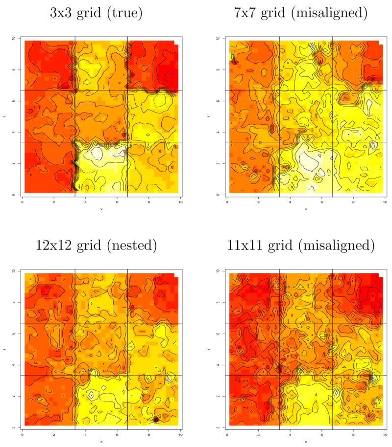
Image plots of estimated spatial effects w(s), the sum of macro-level and micro-level spatial residuals, data simulated from a 3×3 grid.

4.2 Minnesota breast cancer treatment data

In this section, we apply our model to the preliminary Minnesota breast cancer data, introduced in Figure 1. A feature of this data set is that exact addresses are not available for some patients, who are instead assigned to some “central” location in their zip code of residence. As a result, our 3661 patients are recorded as residing at only 3120 unique locations. We experimented with a variety of categorized versions of the minimum distance to RTF covariate, and settled on grouping the minimum distances into three categories: 0 to 30 miles, 30 to 60 miles, and greater than 60 miles. We remark that the two-category (binary) covariate obtained by combining the first two categories also performs well.

Recall that we are interested in the choice of cancer-directed surgery (mastectomy versus BCS) among patients who live in northern Minnesota, a predominantly rural part of the state. We began with a preliminary nonspatial (but still hierarchical) analysis using glmmPQL. These results indicate that a woman’s age, cancer stage and distance she lives from the closest RTF are significant predictors of her surgery choice, with older women, women with later-stage tumors, and women living further from the nearest RTF being more likely to opt for mastectomy.

We wish to fit a spatial model to these data, but as already mentioned, its sheer size precludes standard MCMC-Bayes indicator kriging. As such, we proceed with fitting the multiresolution hierarchical model described in Section 3. A key issue then is of course the choice of an appropriate subregional grid. The most obvious choice here is to use county as the subregional unit. However, as can be seen in Figure 1, there are several counties with more than 200 locations, and one (St. Louis County, the very large east-central county that is home to the port city of Duluth) with about 1000 locations. For a manageable computational burden, we would like each subregion to have at most 100 unique locations. As such, in what follows those counties with too many locations were further subdivided into clusters of proximate cases by strategic latitudinal and longitudinal slicing. A jittered picture of our final partition is shown in Figure 5, which uses both plotting character and level of shading to indicate subregion membership, and open triangles for the regional empirical centroids. This sliced county map determines a proximity matrix we may use when we adopt a CAR model for the macro-level spatial effects, as in (4). We work with this partition for now, but investigate robustness to this choice below.

Figure 5.

Jittered modified county-level partition of breast cancer treatment data. Within each county, the cases’ subregional index numbers are plotted using a common shading. Open triangles indicate subregional centroids.

We include the fixed effects (age, and the later stage and higher minimum distance to RTF indicator variables) in the x vector, and place a flat prior on the corresponding regression parameter β. The variance parameters ${\sigma }_{\mathit{mac}}^2$ and ${\sigma }_k^2$ are assigned relatively vague inverse gamma priors having shape parameter 2.0 and scale parameter “backed out” by matching the prior mean to the estimates obtained earlier from our glmmPQL routine. This means our approach is empirical Bayes in nature, though the amount of prior information being borrowed from the dataset here is very small, since the prior variance is infinite. We did experiment briefly with a U(0.0001, 10) prior for the variance parameters, as encouraged by Gelman et al. (2004), and while this did cause a small upward shift in these parameters’ posteriors, we did not see significant impact on the spatial range or other parameters of interest. This algorithm also suffered from slightly poorer convergence.

As usual, the spatial correlation parameters (φ’s) are difficult to estimate from the data, so we again think of them as tuning constants. In particular, we compare three cases in which φ_mac and the φ_k are fixed so that the effective spatial range is equal to some predetermined percentile of the corresponding inter-site distances. That is, suppose we want the effective range in region k, 3/φ_k, to be equal to q_r(d_k), the rth empirical percentile of the inter-site distances in region k. We would then set

$${\phi }_k=\frac{3}{q_r(d_k)},\mathrm{\hspace{0.17em} }k=1,\dots ,K.$$

In this paper we consider r = 0.25, 0.5, and 0.75. The value for φ_mac was determined similarly, this time using percentiles of the inter-centroidal distances among all regions.

Our baseline model above uses exponential correlation functions at both the macro and micro levels. However, we also investigated model (4), which replaces the point-level data model for the macro effects with the CAR structure. A further modification altered the micro level correlation function from exponential to Matern, a form widely praised for its flexibility and which contains the exponential as a special case (by setting its smoothness parameter ν = 0.5). Sadly, this extension does not provide significantly better fit to our dataset, while also greatly slowing down the computational process. Specifically, more than 70% of the estimated region-specific Matern smoothness parameters ν_k are between 0.35 and 0.58, suggesting fit similar to that of the exponential model.

Table 3 gives the DIC results under our three r values, as well as the CAR plus exponential model assuming r = 0.5, and the CAR plus Matern model with r = 0.5. Comparing to a simple nonhierarchical logistic model fit entirely at the micro level (indicated by glm in the table) and the same model with nonspatial macro-level random intercepts added (indicated by glmm), all of our models have smaller fit scores D̄, somewhat larger effective sizes p_D, and better (smaller) overall DIC scores. DIC is smallest when setting the two r values to 0.5, indicating some degree of “spatial story” in our data. The effective number of parameters decreases as φ decreases (r increases), also suggesting some level of spatial association.

Table 3.

DIC-based model scores, breast cancer data. Here, r is the percentile of the distances on the map that the effective range equals, and determines the prior value of the range parameters φ_k and φ_mac.

	spatial covariance models		model choice statistics
partition	macro level	micro level	D̄	D(θ̄)	pD	DIC
modified county	Expo(r = 0.25)	Expo(r = 0.25)	4603.39	4542.08	61.31	4664.70
	Expo(r = 0.5)	Expo(r = 0.5)	4561.32	4512.65	48.67	4609.98
	Expo(r = 0.75)	Expo(r = 0.75)	4607.02	4562.44	44.58	4651.61
	CAR	Expo(r = 0.5)	4630.14	4592.10	38.04	4668.18
	CAR	Matern(r = 0.5)	4660.11	4628.57	31.53	4691.64
	glm	—	4712.03	4705.08	6.95	4718.98
	glmm	—	4689.69	4664.54	25.15	4714.85

Table 4 gives parameter estimates for β, ${\sigma }_{\mathit{mac}}^2$ and one of the ${\sigma }_{\mathit{mic},k}^2$ parameters (k = 1) under the multiresolution models. In all our models, we use three distance classifications (driving distance to nearest RTF less than 30, 30–60, or greater than 60 miles) which we index as 1, 2 and 3. Similarly we used four stage classifications, in situ (pre-cancer), local (tumor confined to the breast), regional (tumor spread beyond the breast), and distant (metastasis) which we index as 1, 2, 3, and 4. The intercept in our model thus captures the baseline case of women who have Stage 1 (in situ) cancer and live less than 30 miles from the nearest RTF. MCMC-based results from the nonspatial but hierarchical (glmm) model are also shown for comparison. These were obtained by coding this model in R using the generic multivariate Metropolis routine metrop; parameter estimates obtained from the (non-Bayesian) glmm routine were similar. The effects of age, stage, and Dist 3 (closest RTF more than 60 miles away) remain significant, although there is some attenuation of the Dist3 effect, perhaps due to the incorporation of distance into both this covariate and the error distributions by our Bayesian models. In a similar vein, the Bayesian spatial models better allocate variability to both the macro and micro scale, and suggest that the glmm variance estimate (0.038) may be a bit too low, even though in this model it is supposed to account for both macro- and micro-level variability.

Table 4.

Parameter estimates (standard deviations), breast cancer treatment data. Stage 2 denotes local stage, Stage 3 denotes regional stage, and Stage 4 denotes distant (metastasized) stage; Stage 1 (in situ, or pre-cancer) is the baseline. Dist 2 denotes living between 30 and 60 miles from the nearest RTF; Dist 3 indicates this distance is more than 60 miles; Dist 1 (where this distance is less than 30 miles) is the baseline. Age is patient age at cancer diagnosis, centered around its own mean (64.4 years). Only results for σ_mic,1 are shown; results for the other σ_mic,k were similar. In glmm, ${\sigma }_{\mathit{mac}}^2$ is the variance of random effects on subregions which is the total variance of residuals.

	glmm	r = 0.25	r = 0.50	r = 0.75	CAR+Expo(r = 0.5)
Intercept	0.65(0.11)	0.671 (0.13)	0.648 (0.12)	0.620 (0.13)	0.714 (0.11)
Age	−0.15(0.04)	−0.157 (0.04)	−0.153 (0.04)	−0.153 (0.04)	−0.157 (0.04)
Stage 2	−0.80(0.10)	−0.808 (0.10)	−0.826 (0.10)	−0.798 (0.10)	−0.821 (0.10)
Stage 3	−1.71(0.12)	−1.721 (0.12)	−1.734 (0.12)	−1.712 (0.12)	−1.733 (0.12)
Stage 4	−1.90(0.35)	−1.903 (0.36)	−1.883 (0.36)	−1.912 (0.36)	−1.887 (0.36)
Dist 2	−0.03(0.10)	−0.073 (0.10)	−0.033 (0.10)	−0.016 (0.10)	−0.082 (0.10)
Dist 3	−0.28(0.10)	−0.301 (0.11)	−0.282 (0.10)	−0.254 (0.10)	−0.329 (0.10)
${\sigma }_{\mathit{mac}}^2$	0.038(0.02)	0.053 (0.02)	0.043 (0.02)	0.045 (0.02)	0.036 (0.02)
${\sigma }_{\mathit{mic},1}^2$		0.043 (0.06)	0.042 (0.02)	0.043 (0.02)	0.036 (0.02)

Figure 6 shows an image plot of the estimated spatial residuals, w̄(s_i(k))+ μ_k, under two of our three chosen values for the spatial association parameter r and the combination of CAR with the exponential. The residual surfaces are quite smooth and there are no discernible patterns, except for a persistent anomaly (i.e., a light-shaded peak very close to a dark-shaded valley) toward the northwest part of the state. (This behavior is apparently driven by the cases near the city of Grand Forks, which has an RTF but also lies across the state line in North Dakota.) The Figure 6 plots and those of the micro-level spatial effects w̄(s_i(k)) (not shown) are very similar, suggesting the μ_k are all relatively close to zero. Indeed, the μ_k estimates vary from roughly −0.14 to 0.17, while the w̄ estimates essentially cover the range from −1.5 to 1.5. However, the corresponding maps of the estimated μ_k given in Figure 7 do show a clear pattern, with generally positive (light-shaded; higher chance of BCS) fitted effects in the central and southwestern portions of the study region, and patches of negative (dark-shaded; higher chance of mastectomy) fitted effects in the northwest corner as well as the northeast near the Lake Superior shore. The Bayesian model that fixes r = 0.75 does appear somewhat smoother than the r = 0.25 map (for example, combining the two light shaded modes in the central part of the state into a single mode), but overall the pattern is very similar. The CAR-plus-exponential model also delivers a similar overall pattern, though it is not quite as smooth, perhaps reflecting the additional randomness in r and the local (CAR) spatial model at the macro level. Finally, the last panel of Figure 7 corresponds to the nonspatial glmm model; it appears oversmoothed, though it does still indicate a small pocket of negative fitted effects near Lake Superior. (Note that no glmm map is included in Figure 6 since this model has no micro-level effects.)

Figure 6.

Image plots of estimated spatial residuals, breast cancer treatment data, based on modified county-level partition.

Figure 7.

Image plots of macro-level spatial effects μ_k, breast cancer treatment data, based on modified county-level partition.

The interpretation of the first 3 panels of Figure 7 is that, even after accounting for local variability, the fixed effects portion of the model appears to be slightly underpredicting the number of BCS cases in the lighter regions, and overpredicting in the darker ones. This finding is intriguing for a number of reasons. Many women in the lighter regions live far from an RTF, and therefore might be expected to opt more for mastectomy; this may be a case of the covariate “overcorrecting” in these regions. Conversely, the women living near Lake Superior seem to be opting for mastectomy more than their fixed effects would have suggested, perhaps indicating a lurking socioeconomic or attitudinal covariate.

Our regional grouping of patients is based on a visually informed but still fairly ad hoc refinement of a existing geopolitical regional (county-level) grid. To the extent that pairs of women live near but on opposite sides of a county boundary, this grouping may be suboptimal. As such, we developed a second partition of our dataset using the k-means clustering function kcca in the R package flexclust; see http://cran.r-project.org/src/contrib/Descriptions/flexclust.html. While this approach may deliver a more natural patient grouping, it will not permit unique determination of a regional proximity matrix, hence the CAR model (4) is no longer sensible. Figure 8 shows the (jittered) resulting partition with K = 60 clusters; the resulting n_k range from 9 to 146. This partition is often visually similar to our older, county-based partition, although there are many cross-county clusters. Table 5 is the analog of Table 3, giving DIC-based model choice results under our three r values, as well as the glm and glmm models. The cluster-based partition does lead to somewhat smaller p_D scores, but not to noticeable improvements in DIC score.

Figure 8.

Jittered partition of the breast cancer treatment data using cluster analysis; within each cluster, the cases’ subregional index numbers are plotted using a common shading.

Table 5.

DIC-based model scores, breast cancer data based on clustering grouping. Here, r is the percentile of the distances on the map that the effective range equals, and determines the prior value of the range parameters φ_k and φ_mac.

	spatial covariance models		model choice statistics
partition	macro level	micro level	D̄	D(θ̄)	pD	DIC
k-means clustering	Expo(r = 0.25)	Expo(r = 0.25)	4638.38	4586.52	51.86	4690.23
	Expo(r = 0.5)	Expo(r = 0.5)	4649.27	4612.90	36.37	4685.64
	Expo(r = 0.75)	Expo(r = 0.75)	4637.59	4600.76	36.83	4674.43
	glm	—	4712.08	4705.09	6.99	4719.08
	glmm	—	4681.32	4655.39	25.94	4707.26

Table 6 is the analog of Table 4, and shows the main effect estimates under this new k-means-based clustering partition. The main effect estimates are consistent with our previous results; in particular, the primary covariate of interest (Dist3) is largely unchanged despite the reorientation of the regions. Figure 9 maps the estimated macro-level spatial effects. Notice that the north-central region appears somewhat different from that arising from our modified county partition in Figure 7. A possible reason for this is the paucity of subjects in that area, which is no longer a single large region corresponding to Koochiching County (the large north central county that is home to a cluster of cases in International Falls, a city on the Canadian border). We also notice a difference in the southwest corner. Again, some clusters in this area are now narrow slices (instead of rectangles), which may well have caused this difference.

Table 6.

Parameter estimates (standard deviations), breast cancer treatment data based on cluster grouping. Note that ${\sigma }_{\mathit{mic},1}^2$ is not comparable to that in Table 4 since they do not refer to the same set of sugregions.

	glmm	r = 0.25	r = 0.5	r = 0.75
Intercept	0.66(0.11)	0.665 (0.12)	0.65 (0.13)	0.68 (0.12)
Age	−0.15(0.04)	−0.15 (0.04)	−0.16 (0.04)	−0.16 (0.04)
Stage 2	−0.80(0.10)	−0.810 (0.10)	−0.80 (0.11)	−0.81 (0.10)
Stage 3	−1.70(0.12)	−1.718 (0.12)	−1.72 (0.12)	−1.73 (0.12)
Stage 4	−1.88(0.35)	−1.908 (0.36)	−1.91 (0.36)	−1.91 (0.37)
Dist 2	−0.08(0.10)	−0.059 (0.10)	−0.11 (0.10)	−0.11 (0.10)
Dist 3	−0.28(0.11)	−0.266 (0.11)	−0.26 (0.11)	−0.25 (0.11)
${\sigma }_{\mathit{mac}}^2$	0.048(0.02)	0.058 (0.02)	0.041 (0.02)	0.044 (0.02)
${\sigma }_{\mathit{mic},1}^2$		0.043 (0.01)	0.032 (0.01)	0.043 (0.03)

Figure 9.

Image plot of macro-level spatial effects μ_k, breast cancer treatment data based on the cluster grouping.

Finally, Figure 10 shows an image plot of the macro-level spatial effects μ_k from slightly more general models that do not fix the r parameters, but instead place priors on them. In particular, the “Expo+Expo” model uses exponential priors for both the macro and micro levels, with the priors on φ determined as above. Likewise, the “CAR+Expo” model switches to a CAR model at the macro level, but maintains the exponential micro model. The last two panels in the figure replace one or both of these specifications with Matern models, where the prior on φ is again the same as above, and the prior for the smoothing parameter ν is taken to be Unif(0.2, 1). The CAR results appear slightly smoother, as we might expect. The Matern model does not appear dramatically different from the exponential results, suggesting that our simpler, exponential models may be adequate here.

Figure 10.

Image plot of macro-level spatial effects μ_k from general model, breast cancer treatment data based on the modified county grouping.

5 Discussion and future work

In this paper, we introduced a variety of multilevel models that remain feasible for large spatial datasets when traditional MCMC methods are precluded by the need to repeatedly invert high-dimensional matrices. We illustrated with both simulated and real data, and showed a reasonable degree of robustness of the posteriors of interest to the precise choice of the regional grid. Substantively, our findings are important for understanding breast cancer treatment choices in northern Minnesota. The effect of living more than 60 miles from the nearest RTF on the probability of receiving BCS is near −0.3 on the logit scale. That is, the logit of the probability of receiving BCS is 0.3 units lower for women who live more than an hour’s drive from the nearest RTF. Converting back to the probability scale using the point estimates from the best-fitting (r = 0.50) model in Table 4 and setting the macro and micro random effects equal to 0, we can estimate BCS selection probabilities for typical women in the study having certain covariate values. For instance, a typical woman aged 40 with Stage 1 (in situ) cancer who lives fewer than 30 miles from the nearest RTF chooses BCS with probability 0.714; if her driving distance is more than 60 miles, this probability drops to 0.653. At the other extreme, for a typical woman aged 80 with Stage 4 (metastasized) cancer living fewer than 30 miles from the nearest RTF, the BCS selection probability is just 0.197; if her driving distance is more than 60 miles, this probability further drops to 0.156.

In addition, the regional effects μ_k are interesting in their own right, since they indicate areas of unusually high or low BCS rates that are not explained by age, stage, or distance to RTF. Thus our area-based analyses so far confirm the relationship between traveling distance and a decreased likelihood of receiving BCS, although there are areas where the current model slightly over- or under-predicts the receipt of BCS. When the data set is finalized (with final data on type of treatment received and complete information on residence at diagnosis), these results could change, but we do not expect a marked change in our major findings.

Substantively, our primary objective was a practical strategy for assessing the connection between location of residence and therapeutic decision for breast cancer while accounting for underlying spatial effects. As such, we adopted a flexible hierarchical framework that deliberately avoided complicated reversible jump MCMC algorithms. However, one could envision using such an approach to account for uncertainty in the proper partitioning of our spatial domain. Since such algorithms often run into convergence problems that are difficult to resolve, we opted instead to investigate the sensitivity of our results over a few partitions. Our findings indicate some sensitivity to both model and partition at the random effect level (see Figures 7 and 9), but nothing that alters the significance of the primary quantity of interest, a 60 mile or greater distance to nearest RTF (see Tables 4 and 6).

Additional data on covariates would also be useful. For example, factors such as the presence of multifocal disease in the breast (which is a relative contraindication for BCS, again according to the NCI website), and the presence of co-morbidities will affect the choice of cancer-directed therapy. The time of year when radiation therapy would have been given may also affect the type of surgery a person receives (winter travel in rural, northern Minnesota can be risky). Although BCS is sometimes used in advanced-stage breast cancer, it is not usually directed at a cure (distant metastases have already occurred), so exclusion of advanced-stage (stage IIIB, inoperable IIIC, and IV) breast cancer from the models may improve their predictive ability.

Health care utilization is affected by socioeconomic status (e.g., income, blue collar or not, education, etc.) which is not available at the individual level but can be estimated from census tract or census block group (Krieger et al., 2002), and so future work may examine these factors. In addition, patients’ race affects health care utilization, but there are too few non-whites in rural Minnesota to do an area-based analysis. Another question we hope to examine is how distance to RTF is associated with whether or not a woman receives radiation therapy following BCS.

In terms of extending our statistical methodology to improve or robustify our analysis, several possibilities come to mind. These include trying different grids, based on either different geopolitical boundaries (e.g., zip codes) or different clustering algorithms. Robustness to the choice of prior distribution is an important part of any Bayesian data analysis; we have mostly skirted this issue by using noninformative priors whenever possible, but just how “noninformative” they are should perhaps be more thoroughly investigated.

Our current models can also be generalized into a framework that models the spatial effect w(s_i(k)) as a shifted linear combination of random effects with unit variance, i.e. $w({\mathbf{s}}_{i(k)})={\mu }_{ik}+{\sum }_{j=1}^{n_k}{a}_{ij}(k)v_{jk}$, i = 1, …, n_k, where μ_ik’s are the mean effects, υ_jk represents the random effect associated with subject j in region k, and a_ij(k) is the corresponding coefficient. This framework encompasses the “knot-based” methods of Kamman and Wand (2003), where the υ_jk’s are i.i.d. N (0, 1), and also the so-called “coregionalization” methods in geostatistics (Banerjee et al., 2004, Sec. 7.2) where the υ_jk’s themselves arise as spatial process realizations. The identifiability issues that arise in such models can be resolved by modeling the coefficients a_ij(k) for each region k as functions of a micro-level correlation matrix, and Bayesian specifications would again lead to full inference for all association parameters. Models arising from this framework will also involve n_k × n_k matrix computations thereby offering computational feasibility, but the association structures that result are more difficult to interpret. Rather than the simpler additive structure in Section 3, these yield complex multiplicative structures that are extensions of separable models and are useful when the primary concern is the modeling of different spatial ranges or smoothness parameters. Our approach is simpler, yet accommodates the possibility of locally varying spatial association structures through the micro-level modeling.

References

- Banerjee S, Carlin BP, Gelfand AE. Hierarchical Modeling and Analysis for Spatial Data. Boca Raton, FL: Chapman and Hall/CRC Press; 2004. [Google Scholar]
- Banerjee S, Finley AO. Bayesian multi-resolution modelling for spatially replicated datasets with application to forest biomass data. To appear. Journal of Statistical Planning and Inference 2007 [Google Scholar]
- Carlin BP, Louis TA. Bayes and Empirical Bayes Methods for Data Analysis. 2. Boca Raton, FL: Chapman and Hall/CRC Press; 2000. [Google Scholar]
- Celeux G, Forbes F, Robert CP, Titterington DM. Deviance information criteria for missing data models (with discussion) Bayesian Analysis. 2006;1:651–706. [Google Scholar]
- Chiles JP, Delfiner P. Geostatistics: Modeling Spatial Uncertainty. New York: Wiley; 1999. [Google Scholar]
- Cormen TH, Leiserson CE, Rivest RL, Stein C. Introduction to Algorithms. 2. Boston: MIT Press and McGraw-Hill; 2001. [Google Scholar]
- Cressie NAC. Statistics for Spatial Data. 2. New York: Wiley; 1993. [Google Scholar]
- Fang KT, Kotz S, Ng KW. Symmetric Multivariate and Related Distributions. London: Chapman and Hall; 1990. [Google Scholar]
- Finley AO, Banerjee S, McRoberts RE. A Bayesian approach to multi-source forest area estimation. To appear. Environmental and Ecological Statistics 2007 [Google Scholar]
- Fuentes M. Periodogram and other spectral methods for nonstationary spatial processes. Biometrika. 2002;89:197–210. [Google Scholar]
- Fuentes M. Approximate likelihood for large irregularly spaced spatial data. J Amer Statist Assoc. 2007;102:321–331. doi: 10.1198/016214506000000852. [DOI] [PMC free article] [PubMed] [Google Scholar]
- Gelfand AE, Kottas A, Maceachern SN. Bayesian nonparametric spatial Dirichlet modeling with Dirichlet process mixing. J Amer Statist Assoc. 2005;100:1021–1035. [Google Scholar]
- Gelman A, Carlin JB, Stern HS, Rubin DB. Bayesian Data Analysis. 2. Boca Raton, FL: Chapman and Hall/CRC Press; 2004. [Google Scholar]
- Green PJ. Reversible jump Markov chain Monte Carlo computation and Bayesian model determination. Biometrika. 1995;82:711–732. [Google Scholar]
- Higdon D. Space and space time modeling using process convolutions. In: Anderson C, Barnett V, Chatwin PC, El-Shaarawi AH, editors. Quantitative Methods for Current Environmental Issues. London: Springer-Verlag; 2002. pp. 37–56. [Google Scholar]
- Kamman EE, Wand MP. Geoadditive models. Applied Statistics. 2003;52:1–18. [Google Scholar]
- Krieger N, Chen JT, Waterman PD, Soobader MJ, Subramanian SV, Carson R. Geocoding and monitoring of US socioeconomic inequalities in mortality and cancer incidence: does the choice of area-based measure and geographic level matter?: The Public Health Disparities Geocoding Project. Amer J Epidemiology. 2002;156:471–482. doi: 10.1093/aje/kwf068. [DOI] [PubMed] [Google Scholar]
- Lawson AB. Statistical Methods in Spatial Epidemiology. New York: Wiley; 2001. [Google Scholar]
- Lie-Quan L, Lumsdaine A, Siek JG. Boost Graph Library. Addison-Wesley; Professional: 2001. [Google Scholar]
- Møller J, Waagepetersen R. Statistical Inference and Simulation for Spatial Point Processes. Boca Raton, FL: Chapman and Hall/CRC Press; 2004. [Google Scholar]
- Paciorek CJ. Computational techniques for spatial logistic regression with large datasets. Computational Statistics and Data Analysis. 2007;51:3631–3653. doi: 10.1016/j.csda.2006.11.008. [DOI] [PMC free article] [PubMed] [Google Scholar]
- Palacios MB, Steel M. Non-Gaussian Bayesian geostatistical modelling. J Amer Statist Assoc. 2006;101:604–618. [Google Scholar]
- Schabenberger O, Gotway CA. Statistical Methods for Spatial Data Analysis. Boca Raton, FL: Chapman and Hall/CRC Press; 2004. [Google Scholar]
- Scheiner SM, Gurevitch J. Design and Analysis of Ecological Experiments. 2. Oxford UK: Oxford University Press; 2001. [Google Scholar]
- Spiegelhalter DJ, Best NG, Carlin BP, van der Linde A. Bayesian measures of model complexity and fit (with discussion) J Roy Statist Soc, Ser B. 2002;64:583–639. [Google Scholar]
- Stein ML. Interpolation of Spatial Data: Some Theory for Kriging. New York: Springer; 1999. [Google Scholar]
- Ver Hoef JM, Cressie NAC, Barry RP. Flexible spatial models based on the fast Fourier transform (FFT) for cokriging. Journal of Computational and Graphical Statistics. 2004;13:265–282. [Google Scholar]
- Waller LA, Gotway CA. Applied Spatial Statistics for Public Health Data. New York: Wiley; 2004. [Google Scholar]
- Webster R, Oliver MA. Geostatistics for Environmental Scientists. New York: John Wiley and Sons; 2001. [Google Scholar]
- Whittle P. On stationary processes in the plane. Biometrika. 1954;41:434–449. [Google Scholar]
- Wikle C. Spatial modeling of count data: A case study in modelling breeding bird survey data on large spatial domains. In: Lawson A, Denison D, editors. Spatial Cluster Modelling. CRC/Chapman and Hall; 2002. pp. 199–209. [Google Scholar]
- Zhao Y, Staudenmayer J, Coull BA, Wand MP. General design Bayesian generalized linear mixed models. Statistical Science. 2006;21:35–51. [Google Scholar]