Reproducibility of Quantitative Tractography Methods Applied to Cerebral White Matter

Abstract

Tractography based on diffusion tensor imaging (DTI) allows visualization of white matter tracts. In this study, protocols to reconstruct eleven major white matter tracts are described. The protocols were refined by several iterations of intra- and inter-rater measurements and identification of sources of variability. Reproducibility of the established protocols was then tested by raters who did not have previous experience in tractography. The protocols were applied to a DTI database of adult normal subjects to study size, fractional anisotropy (FA), and T₂ of individual white matter tracts. Distinctive features in FA and T₂ were found for the corticospinal tract and callosal fibers. Hemispheric asymmetry was observed for the size of white matter tracts projecting to the temporal lobe. This protocol provides guidelines for reproducible DTI-based tract-specific quantification.

Introduction

Three-dimensional tract reconstruction (tractography) based on diffusion tensor imaging (DTI) is becoming a widely-used tool to study human white matter anatomy (Basser et al., 2000; Conturo et al., 1999; Jones et al., 1999b; Lazar et al., 2003; Mori et al., 1999; Mori et al., 2005; Parker et al., 2002; Poupon et al., 2000). This technology allows us to visualize trajectories of specific white matter fiber bundles and has potential to perform quantitative evaluation of properties of individual tracts. This provides exciting opportunities to assess the impact of diseases on specific white matter tracts. Once the location of a tract is defined, its size can be measured. Further, by superimposing tract coordinates on various MR parameter maps such as T₁, T₂, magnetization transfer ratio (MTR), and diffusion anisotropy, the myelination and axonal status of individual tracts may be monitored (Glenn et al., 2003; Pagani et al., 2005; Partridge et al., 2004; Stieltjes et al., 2001; Virta et al., 1999; Wilson et al., 2003; Xue et al., 1999). However, questions remain whether the tractography results reflect true neuroanatomical details and are sufficiently reproducible to be used as a tool for quantitative analyses.

In terms of validity, there is mounting evidence that tracking results of many prominent white matter tracts agree very well with classical definitions based on postmortem studies (Basser et al., 2000; Catani et al., 2002; Conturo et al., 1999; Jellison et al., 2004; Mori et al., 1999; Mori et al., 2002; Poupon et al., 2000; Stieltjes et al., 2001; Wakana et al., 2004). On the other hand, it is well-known that the technique can produce false positive and false negative results due to noise, partial volume effects, and complex fiber architectures within a pixel (Pierpaoli et al., 2001; Wiegell et al., 2000). One way to raise the confidence level of validity is to employ anatomical constraints by employing multiple regions of interest (ROIs) (Conturo et al., 1999; Huang et al., 2004). This technique requires a priori knowledge about the trajectory and can be used only for well-characterized white matter tracts. This approach should reduce the number of false positive, but is unlikely to be 100% accurate.

While it is difficult to completely characterize the validity of tractography, we can measure its reproducibility. If we can develop a scheme to reproducibly define coordinates of specific white matter tracts, this technique should be a valuable tool to test hypotheses as to whether any of these specific tracts are involved in the disease of interest. Within a given set of imaging parameters, we expect reconstruction reproducibility to vary among white matter tracts depending on their size and trajectory. Therefore, it is important to establish reproducible tracking protocols.

One of the major sources of variability, in addition to noise and partial volume effects, comes from placement of reference ROIs to identify specific white matter tracts. By devising clever ROI drawing schemes, which are based on anatomical features of individual tracts and using regions that are sufficiently large, it is possible to come up with a robust protocol that is rather insensitive to small variations in the ROI drawing (Huang et al., 2004). The protocol can be iteratively improved by measuring intra and inter-rater variability and by identifying and describing the source of variations. The purpose of this paper is to develop such robust protocols and identify white matter tracts that can be reconstructed reproducibly. The reproducibility was characterized by spatial matching among different trials by the same rater (intra-rater) and multiple raters (inter-rater) using the same subject (inter-measurement). In the second part of the study we applied the established protocols to measure size, fractional anisotropy, and T₂ of each tract using our normal DTI database. This study leads to multi-parametric mapping of the normal white matter and the range of normal variations in a tract-by-tract basis.

Methods

Subjects

The study was approved by the institutional review board and informed consents including a HIPAA compliant data sharing agreement were obtained from all subjects. Ten healthy adults (mean 26.1 +/− 5.48 years old, male 5, female 5) participated. All subjects were free of current and past medical or neurological disorders. The raw and processed image data are accessible through our websites (lbam.med.jhmi.edu, godzilla.kennedykrieger.org and www.nbirn.net).

Imaging

A 1.5T MR unit (Gyroscan NT, Philips Medical Systems) was used. DTI data were acquired using single-shot echo-planar imaging with sensitivity encoding (SENSE, parallel–imaging factor, 2.5) (Pruessmann et al., 1999). The imaging matrix was 96 × 96 with field of view of 240 × 240 mm (nominal resolution, 2.5mm), zerofilled to 256 × 256 pixels. Transverse sections of 2.5 mm thickness were acquired parallel to the anterior commissure/posterior commissure line. A total of 50-55 sections covered the entire cerebrum and brainstem without gaps. Diffusion weighting was encoded along 30 independent orientations (Jones et al., 1999a) using a b-value of 700 mm²/s. Five additional images with minimal diffusion weighting (b = 33mm²/sec) were also acquired. The scanning time per dataset was approximately 6 minutes including 2 minutes image reconstruction delay. To enhance the signal-to-noise ratio, imaging was repeated 3 times. Co-registered Magnetization-Prepared Rapid Gradient Echo (MPRAGE) images of the same resolution were recorded for anatomical guidance.

Single-shot-EPI, T2-weighted imaging (TR 4000msec, TEs 40 msec and 100 msec; image resolution and SENSE factor equal to DTI) was performed for T2 quantification. To ensure the best registration between DTI and T₂-weighted images, the same number of echoes was acquired after each excitation.

Data processing

The DTI datasets were transferred to a PC with windows platform and processed using the analysis software DTIstudio developed and distributed by this laboratory (H. Jiang & S. Mori, Johns Hopkins University and Kennedy Krieger institute, http://godzilla.kennedykrieger.org or http://lbam.med.jhmi.edu). Images were first realigned using the AIR program (Woods et al., 1998), in order to remove any potential small bulk motions that occurred during the scans. Subsequently, all diffusion-weighted images were visually inspected for apparent artifacts due to subject motion and instrumental malfunction by authors. The six elements of the diffusion tensor were calculated for each pixel using multi-variate linear fitting. After tensor diagonalization, three eigenvalues and eigenvectors were obtained and fractional anisotropy (FA) maps were calculated. The eigenvector associated with the largest eigenvalue was used as an indicator for fiber orientation. In the DTI color maps, red, green, and blue colors were assigned to right-left, anterior-posterior, and superior-inferior orientations, respectively. T₂ maps were calculated from two separated images with echo times of 40 ms and 100 ms.

Fiber Tracking and ROI drawing strategy

In this study, we investigated the reliability of reconstruction of white matter tracts in each hemisphere. For 3D tract reconstruction, the fiber assignment by continuous tracking or FACT method (Mori et al., 1999; Xue et al., 1999) was used with a fractional anisotropy threshold 0.2 and an inner product threshold of 0.75, which prohibited angles larger than 41 degrees during tracking. The fiber tracking was performed by DTIstudio. A multi-ROI approach was used to reconstruct tracts of interest which exploits existing anatomical knowledge of tract trajectories. Tracking was performed from all pixels inside the brain (brute-force approach) (Conturo et al., 1999; Huang et al., 2004) and results penetrating the manually defined ROIs were assigned to the specific tracts associated with the ROIs. When multiple ROIs were used for a tract of interest, we employed three types of operations, namely “AND”, “CUT”, and “NOT” (Fig. 1), the choice of which depends on the characteristic trajectory of each tract.

Figure 1.

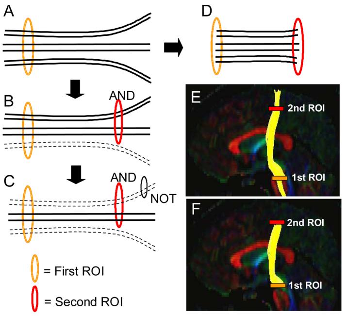
A schematic diagram of three types of ROI operations; AND, NOT, and CUT. When the first ROI is drawn, all tracts that penetrate the ROI are retrieved (A). If the second ROI is applied as an “AND” operation, the fibers that penetrate both ROIs are retained (B). If a “NOT” operation is used, a subset of the fibers penetrating the NOT ROI is removed (C). The CUT operation is similar to the AND operation but only the tracking results between the two ROIs are retained (D). Results of “AND” and “CUT” operations are compared in (E: AND) and (F: CUT) using the corticospinal tract as an example.

In our protocols, two sets of tracking results were generated; one using the “AND” operation (Fig. 1B) and the other using the “CUT” operation (Fig. 1D). For both cases, tracking results that penetrate two ROIs are extracted. When we use the “AND” operation (Fig. 1B, 1E), the results include three sections with different properties; one encompassing the tract before the first ROI (i.e. to the left side in figure 1), one between the two ROIs, and one encompassing the tract after the second ROI (i.e. to the left side in figure 1). Pathways in the middle section are constrained by two destinations with a priori knowledge while the other two sections are not. By using the “CUT” operation, only the middle section is retained (Fig. 1F). Use of the “NOT” operation was sometimes necessary to remove a subset of unwanted projections from a reconstruction result. For identification of anatomical landmarks, color coded maps were used, but certain landmarks, such as sulci, could be more easily identified in co-registered images such as the anisotropy maps and diffusion-weighted images as will be discussed later. In this study, tracts were reconstructed as faithfully as possible based on classical a priori anatomical knowledge from postmortem studies using ROIs that were strategically located based on known fiber trajectories.

Reconstruction protocol

Tract #1: Cingulum cingulate gyrus part (Fig. 2 )

Figure 2.

Locations of the ROIs for the cingulum in the cingulate gyrus part (CGC) on two coronal slices (a and c) and their locations in the mid-sagittal slice (b and d). The SCC and GCC stand for the splenium of corpus callosum and the genu of collupus callosum, respectively.

The cingulum is defined as two separate segments; the upper part along the cingulate gyrus (CGC: cingulum cingulate gyrus part) and lower segment (Tract #2) along the ventral side of the hippocampus (CGH: cingulum hippocampal part).

For CGC (Fig.2), a coronal plane is selected at the middle of splenium of the corpus callosum (CC) using the mid-sagittal plane (Fig.2b) and a ROI as shown in Fig. 2a is drawn. For the second ROI, a coronal plane in the middle of genu of CC is selected using the mid-sagittal plane (Fig. 2d) and a second ROI is drawn to include the cingulum (Fig. 2c). The size of the second ROI doesn't affect the result as long as only the labeled cingulum is included.

Tract #2 ; Cingulum hippocampal part ( Fig. 3 )

Figure3.

Locations of the ROIs for the cingulum in the hippocampal part (CGH ) on two coronal slices (a and c) and their locations in the mid-sagittal slice (b and d).

The inferior segment of the cingulum runs along the ventral aspect of the hippocampus. For the first ROI, a coronal plane in the middle of the splenium of corpus callosum is selected using the mid-sagittal plane (Fig. 3b) and the cingulum below the corpus callosum is delineated. For the second ROI, a coronal slice anterior to the pons is selected using the mid-sagittal plane (Fig. 3d). The second ROI includes the cingulum which is already labeled by the tracking (Fig. 2c).

Tract #3: Cortico-spinal tract (CST) (Fig. 4)

Figure.4.

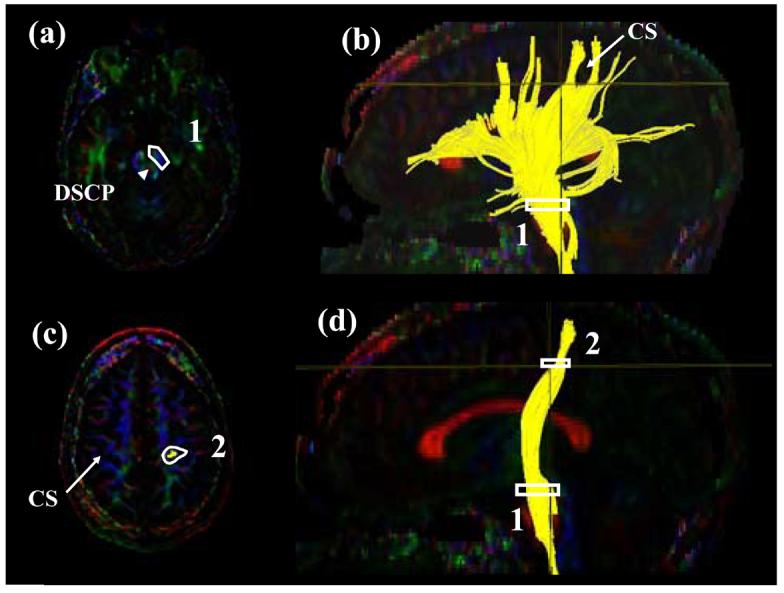
Locations of the ROIs for corticospinal tract (CST) on two axial slices (a and c) and their locations in the mid-sagittal slice (b and d). The first ROI is drawn on the cerebral peduncle at the level of the decussation of the superior cerebellar peduncle (DSCP). From the tracking results, the central sulcus (CS) and the projection to the motor cortex are identified. Using the axial slice right after the bifurcation to the motor and sensory cortex, the CST is selected.

In this protocol, we define the CST between the primary motor cortex and the midbrain. The first ROI defines the entire cerebral peduncle in an axial plane at the level of the decussation of the superior cerebellar peduncle (Fig. 4a), indicated by the arrow. By inspecting the reconstruction result from the first ROI, a bundle of trajectories that reach the primary motor cortex and the location of the central sulcus can be identified. The most ventral axial slice that can clearly identify the cleavage of the central sulcus in the tracking result (Fig. 4b) is selected and the bundle in the primary motor cortex is defined (Figs. 4c and d). As long as only the trajectories to the primary motor cortex are defined, the size of the second ROI can be arbitrary. The trajectories outside the two ROIs may cross the midline via the pontine crossing fibers and re-enter the contralateral hemisphere, which interferes with subsequent quantification procedures. These tracts should be removed by using the “NOT” operation across the entire mid-sagittal slice. Please note that if the “CUT” operation is used, which retains only coordinates between the two ROIs, this extra editing procedure using the “NOT” operation is unnecessary.

The tracking method described in this protocol usually reconstructs only the CST projecting to the medial cortical regions. The CST projection to the lateral areas of motor cortex can not be accurately reconstructed because there is a significant mixing of fibers with different orientations within the pixels as the CST passes through the massive bundle of association fibers.)

Tract #4: Anterior Thalamic Radiation (ATR) (Fig. 5)

Figure 5.

Locations of the ROIs for anterior thalamic radiation (ATR) on two coronal slices (a and c) and their locations in the mid-sagittal slice (b and d). The IC stands for the internal capsule.

A coronal slice is selected at the middle of the genu of corpus callosum (Fig. 5a, b). The first ROI defines the anterior limb of internal capsule (Fig.5 a). For the second ROI, a coronal plane at the anterior edge of pons (Fig.5 d) is selected and the entire thalamus is delineated (Fig.5 c). The trajectories outside the two ROIs may cross the corpus callosum and enter the contralateral hemisphere. These trajectories are removed by a “NOT” operation across the entire mid-sagittal slice.

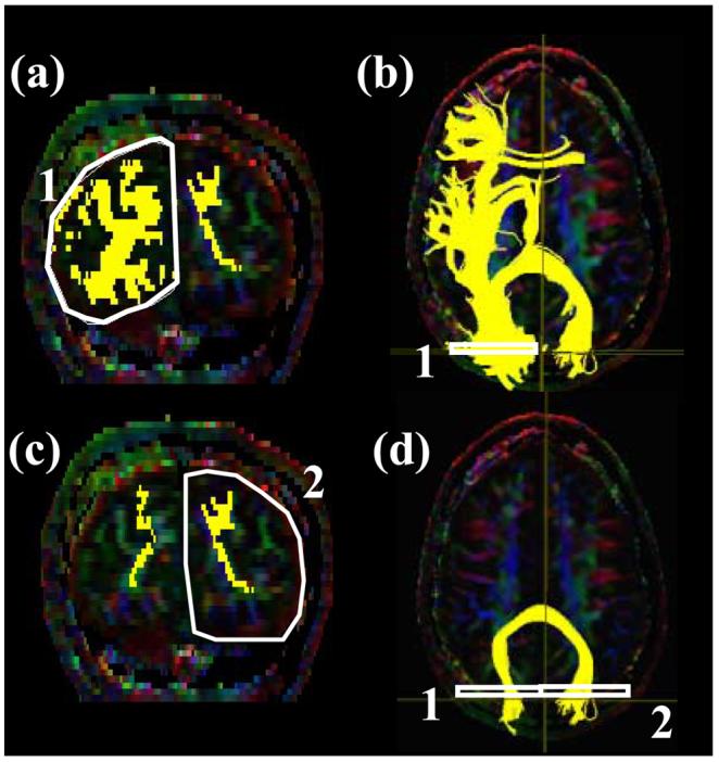
Tract #5: Superior Longitudinal Fasciculus (SLF) (Fig. 6)

Figure 6.

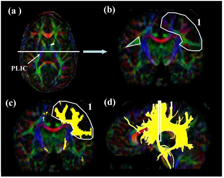
Locations of the ROIs for superior longitudinal fasciculus (SLF). At the middle of the posterior limb of the internal capsule (a, PLIC), a coronal slice is selected (b). The SLF can be identified as an intense triangle-shape green structure. The first ROI is shown in (c: coronal) and (d: sagittal). For the second ROI, a coronal slice (e) is selected at the splenium of corpus callosum (f). For the temporal component of the SLF (SLFt), the second ROI is drawn on the axial slice at the anterior commissure (AC) level (g and h). The SS stands for the sagittal stratum.

We tested two different protocols to define the SLF. One is used to reconstruct the SLF as comprehensively as possible and the other is selective for isolating the trajectories to the temporal lobe (named SLFt in this paper).

For the 1st ROI, the lowest axial level in which the fornix can be identified is selected as a single intense structure (Fig. 6a, the fornix is indicated by an arrowhead). Then a coronal slice is selected at the middle of the posterior limb of internal capsule (Fig.6 a; white line). The core of the SLF can be identified as an intense green tract with a triangular shape (Fig. 6b, white triangle). The first ROI includes this core and all branches coming out from the triangular area (Fig. 6b and 6c).

For the second ROI, a coronal slice is selected at the middle of the splenium of corpus callosum using the mid-sagittal level (Fig. 6e and 6f). The second ROI includes all labeled fibers (Fig. 6e).

Tract #6: The temporal component of the SLF (Fig.6)

For the temporal component of SLF (SLFt), the first ROI is same as the body of SLF. For the second ROI, an axial slice is selected at the level of the anterior commissure (AC in Fig. 6g) and the projections located laterally to the sagittal stratum (SS in Fig. 6g) are delineated by the second ROI.

Tract #7: Inferior longitudinal fasciculus (ILF) (Fig.7)

Figure 7.

Locations of the ROIs for the inferior longitudinal fasciculus (ILF). First a para-sagittal plane (b) is identified at the level of the cingulum (a, CG). The parieto-occipital sulcus (POS) is identified in the sagittal plane. The least-diffusion-weighted image could be used as a better anatomical guidance to identify the POS. A coronal slice (c and d) is selected at the posterior edge of the cingulum (slice #1). The second ROI defines trajectories toward the anterior pole of the temporal lobe (e and f).

Using a parasagittal slice, the posterior edge of the cingulum is identified (Fig. 7b, indicated by an arrow). A coronal slice is selected at that edge (coronal level #1 in Fig. 7b). The first ROI includes the entire hemisphere (Fig. 7c). For second ROI, the most posterior coronal slice in which the temporal lobe is not connected to the frontal lobe is selected (Fig. 7e). The second ROI includes the entire temporal lobe.

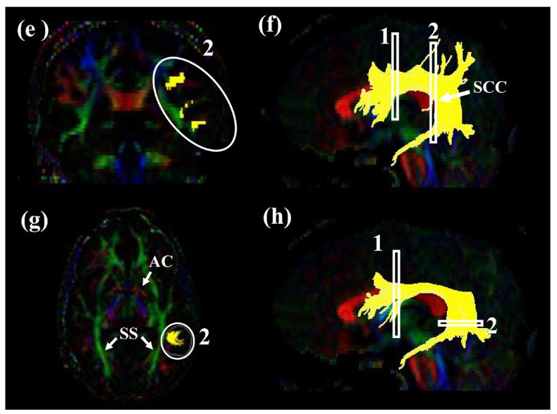
Tract #8: Inferior fronto-occipital fasciculus (IFO) (Fig 8)

Figure 8.

Locations of the ROIs for the inferior fronto-occipital fasciculus (IFO) on two coronal slices (a and c) and their locations in the mid-sagittal slice (b and d). For the coronal slice in (a), the #2 slice in Fig. 7b is used.

For the first ROI, a coronal slice (the coronal level #2 in Fig.7b) is identified at the middle point between the posterior edge of the cingulum (slice level #1 in Fig. 7b) and the posterior edge of the parieto-occipital sulcus (slice level #3 in Fig. 7b). Although a color map is shown in Fig. 7b, another anatomical image such as the least-diffusion-weighted image better defines the parieto-occipital sulcus. The first ROI delineates the occipital lobe. The boundary between the occipital and parietal lobes is defined by linearly extrapolating the parieto-occipital sulcus (POS) to the lateral region (Fig. 8a). For the second ROI, a coronal slice is selected at the anterior edge of the genu of corpus callosum (Fig. 8c) and the entire hemisphere is delineated. These two ROIs are sometimes shared by the cingulum and some fibers relayed at the thalamus. These fibers clearly don't belong to the IFO and should be manually removed using “NOT”.

Tract #9: Uncinate fasciculus (UNC) (Fig.9)

Figure 9.

Locations of the ROIs for the uncinate fasciculus (UNC) on a coronal slice (a and c) and their locations in the mid-sagittal slice (b and d). The coronal slice (a and c) is the most posterior slice where the frontal and temporal lobe is separated. The least-diffusion-weighted image could be used for better anatomical guidance.

The most posterior coronal slice in which the temporal lobe is separated from the frontal lobe is selected (Figs. 9a and 9c). The first ROI includes the entire temporal lobe and the second ROI includes the entire projections toward the frontal lobe.

Tract #10: The forceps major (Fmajor) (Fig.10)

Figure 10.

Locations of the ROIs for the occipital projection of the corpus callosum (forceps major, FMajor) on a coronal slice (a and c) and their locations in an axial slice (b and d). For the coronal slice in (a) and (b), the #3 slice in Fig. 7b (posterior edge of the POS) is used.

It is difficult to devise a protocol that can reconstruct the entire corpus callosum reproducibly. In this paper, reconstruction of callosal connections to the occipital lobe via the splenium of corpus callosum (forceps major) and to the frontal lobe via the genu of corpus callosum (forceps minor) are devised.

For the 1st ROI for the forceps major (Fmajor), a para-sagittal plane at the level of cingulum is selected (Fig.7a) and the parieto-occipital sulcus is identified. A coronal plane is selected at the most posterior edge of this sulcus (coronal slice #3 in Fig. 7b) so that the coronal plane includes only the occipital lobe. The least-diffusion-weighted image may be used for better identification of the sulcus. The first and second ROIs delineate right and left occipital lobe as shown in Fig. 10a and 10c.

Tract #11: The frontal projection of the corpus callosum (the forceps minor) (Fminor) (Fig.11)

Figure 11.

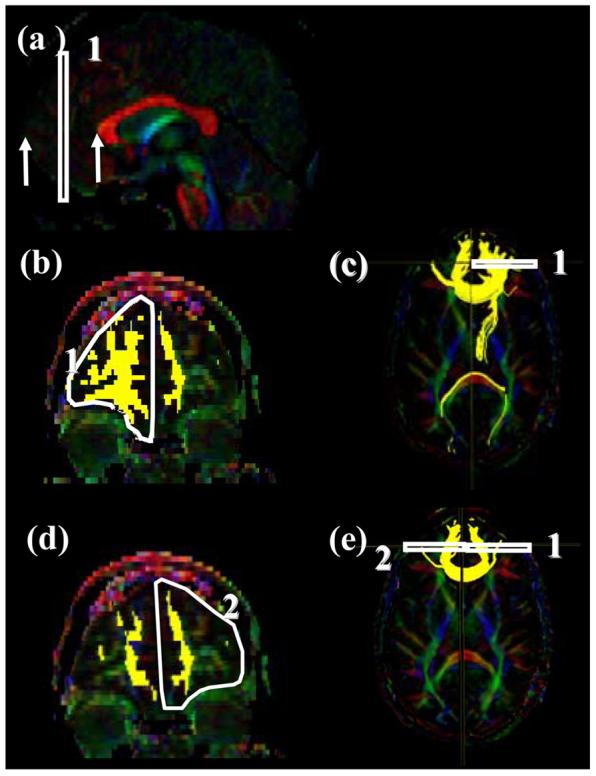
Locations of the ROIs for the frontal projection of the corpus callosum (forceps minor, FMinor) on a sagittal slice (a), a coronal slice (b and d) and their locations in an axial slice (c and e).

For the first ROI (Fig.11b), a coronal plane at the middle point between the anterior tip of frontal lobe and the anterior edge of the genu of the CC is selected using the mid-sagittal plane (Fig. 11a, between the two arrows). The first and second ROIs delineate the entire frontal lobe of each side as shown in Fig. 11b and 11d).

Reproducibility measurements

To quantify the reproducibility of the fiber tracking protocol, intra-rater and inter-rater reproducibility was assessed. The 11 protocols were repeated three times by an operator for the intra-rater reproducibility. For inter-rater reproducibility, the protocols were performed by three different operators using the same data set (called Subject #1 hereafter). Three raters participated within the same institute (S.W., P.D., and A.B at JHU). Protocols that passed the initial intra-institutional reproducibility tests (kappa values more than 0.6) were passed to 3 additional raters in 3 different institutes (A.C. at UNM, M.P. at UCSD, and M.P. at UCI), to measure inter-institutional reproducibility. The entire procedure was repeated using two more datasets from different subjects (Subject #2 and Subject #3) and the results were averaged. The 3 raters outside JHU didn't have prior experience in tractography and their training and instruction was accomplished independently using the written protocols. Therefore, the inter-institutional reproducibility could be considered as the poorest reproducibility condition; but the one that most accurately reflects the state of the field.

Statistical Analysis of spatial matching by κ

Spatial matching was examined for statistical analysis of reproducibility. The repeated tracking results were first converted to binary information of the same pixel dimension as the DTI data (256×256×50), in which pixels that were occupied by the tracts were assigned to a value of 1 and other non-occupied pixels were assigned to a value of 0. Two tracking results out of 3 trials were then superimposed, which yields to four different pixel categories; (1) pixels did not contain the tract in both trials (nn), (2) pixels that contained the tract in only one of the two trials (pn, np), and (3) pixels that contained the tracts in both trials (pp). Expectation values (Enn, Enp, Epn, and Epp) for each class were then calculated using the equations;

$$\text{Expected nn}\left(\text{Enn}\right)=(\text{nn}+\text{np})(\text{nn}+\text{pn})∕\text{N}$$

$$\text{Expected np}\left(\text{Enp}\right)\text{or Epn}=(\text{nn}+\text{np})(\text{np}+\text{pp})∕\text{N or}(\text{nn}+\text{pn})(\text{pn}+\text{pp})∕\text{N}$$

$$\text{Expected pp}\left(\text{Epp}\right)=(\text{pn}+\text{pp})(\text{np}+\text{pp})∕\text{N}$$

Where N=nn+np+pn+pp is the total number of pixels for the particular fiber. For the calculation, pixels with FA lower than the threshold (FA > 0.2) were not included. Then κ (kappa) was calculated by κ = (observed agreement − expected agreement)/ (100− expected agreement), where

$$\text{observed agreement}=(\text{nn}+\text{pp})∕{\text{N}}^{\ast }100$$

$$\text{expected agreement}=(\text{Enn}+\text{Epp})∕{\text{N}}^{\ast }100$$

This analysis was applied in a pair-wise manner; there are three combinations from the 3 trials. The κ values were determined for the three pair-wise combinations and an average κ was determined. According to criteria set by Landis and Koch (1977), the κ value of 0.11-0.2 is considered as “slight,” 0.21-0.4 as “fair”, 0.41-0.60 as “ moderate”, 0.61-0.80 as “substantial ”, and 0.81-1.0 as “ almost perfect” agreement.

Study of tract-specific MR parameters in the normal subjects

The protocols with high reproducibility were applied to the normal population (n = 10) and coordinates of each of the white matter tracts were identified. These coordinates were superimposed on FA, and T₂ maps to measure these parameters in a tract-specific manner. The tract size was also calculated from the number of pixels occupied by the tracts.

These results were represented in two different ways. First, the all occupied pixels were pooled to determine the average parameter value for each tract. Second, the parameters were projected onto one of the anatomical axes (right-left, anterior-posterior, and superior-inferior) to observe changes in the parameters along the course of the trajectory. For inter-subject averaging, the tract length was normalized using anatomical landmarks along its course. For example, the CST was segmented into the midbrain, internal capsule, and corona radiate regions. The length of these separate regions from each subject was linearly adjusted before group averages were calculated.

Results

1: Intra and inter-rater reproducibility

Table 1 shows κ values of intra and inter-rater reproducibility (3 raters within an institute), inter-institutional reproducibility (3 raters, one each from three different institutes for Subject #1-1 and Subject #1-2 data), and average results for three different datasets (3 raters from three institutes for Subject #1, Subject #2, and Subject #3 data). For the 11 fibers with the established protocol, κ values are always higher than 0.6, and mostly higher than 0.7. As expected, inter-institutional reproducibility tends to be poorer than other reproducibility measures. Differences between the “AND” and “CUT” operations are unexpectedly small, with reproducibility of “CUT” operation often lower than that of “AND”. This is because the tract definition for the “CUT” operation is sensitive to the locations of ROIs, especially when two ROIs are close together (e.g. SLF). In these cases, a one-slice shift of the ROI location leads to addition or subtraction of a group of pixels within the slice and has a large effect on the κ value.

Table 1.

The k value of Intra- and Inter- rater Variability for the Eleven Major Tracts

		CGC	CGH	CST	ATR	SLF	SLFt	ILF	IFO	UNC	Fmaj	Fmin
Intra- rater	AND	0.994	0.992	0.94	0.902	0.982	0.944	0.974	0.985	0.996	0.976	0.983
	CUT	0.989	0.955	0.952	0.919	0.938	0.914	0.94	0.942	0.989	0.955	0.952
Inter- rater	AND	0.968	0.814	0.797	0.763	0.888	0.913	0.694	0.882	0.919	0.932	0.973
	CUT	0.940	0.911	0.793	0.797	0.727	0.888	0.654	0.893	0.912	0.966	0.975
Inter- Institute	AND	0.884	0.953	0.869	0.870	0.910	0.753	0.823	0.851	0.916	0.645	0.908
	CUT	0.879	0.900	0.787	0.787	0.743	0.695	0.732	0.842	0.810	0.600	0.860
3 subjects average	AND	0.873	0.831	0.889	0.831	0.904	0.745	0.782	0.856	0.758	0.735	0.911
	CUT	0.788	0.818	0.854	0.702	0.741	0.648	0.754	0.815	0.800	0.690	0.873

0.81-1.0 ; almost perfect agreement, 0.61-0.80 ;substantial, 0.41-0.60 ; moderate, 0.21-0.4 ; fair , 0.01-0.2 ; slight

The intra and inter-rater reproducibility of FA measurements were also performed by superimposing each trial result on the FA map. The coefficients of variation (CV = standard deviation/average) for the intra and inter-rater variability are very small for all 11 tracts; the CV averaged over the 11 tracts are 0.8 and 1.5% for intra and inter-rater variability using AND operations and 1.1 and 1.0% using CUT operations.

2: Study of normal population

Averaged sizes of fibers (the number of pixels that contain the fibers multiplied by the nominal size of the pixel) for 10 healthy volunteers are shown in Fig. 12B. The reconstructed tracts tend to be larger in the left hemisphere and the differences are significant for the CGC, SLFt, ILF, and UNC, while no difference is found for CST and IFO. Interestingly all asymmetric tracts are related to the temporal lobe. Please note that these volumes were not normalized for the differences in cranial volumes. The asymmetry results, however, should not be influenced by the normalization. The asymmetry of FA is far smaller and significant difference is found only in CGC (L > R) and CGH (R > L) (Fig. 12A).

Figure 12.

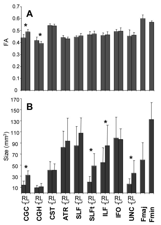
FAs and sizes of white matter tracts of each reconstructed tract in 10 healthy volunteers. Averages and standard deviations of the 10 subjects are shown (the standard deviation reflects the population variance, not the measurement reproducibility). Asterisks indicate statistically significant difference with p < 0.05. R and L indicate right and left hemisphere.

In Fig. 13, a correlation plot between T₂ and FA is shown for each tract. Most tracts are clustered in the T₂ range of 65 – 70 ms and FA range from 0.4 – 0.5. Exceptions are the corpus callosum, featured with a high anisotropy and the corticospinal tract, featured by high anisotropy and long T₂ although the differences were very small (0.02-0.04 in FA).

Figure 13.

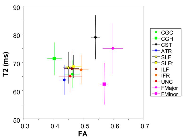
A correlation plot for FA and T₂ of each tract. Most of tracts are clustered in the FA range between 0.4-0.5 and a T2 range between 60-75 ms, except for the CST, FMajor, and FMinor.

Data in Fig. 13 were calculated from all pixels that belong to a tract. The data can be projected to one of the anatomical axes. Fig. 14 shows results of several tracts with characteristic and reproducible variation of T₂ and FA along the course of their trajectories. For example, the CST has relatively high anisotropy in the internal capsule. Relatively long T₂ of the CST is apparent throughout its trajectories, although it has monotonic decrease toward the cortex. The IFO has an area with high FA at coronal slices near the anterior commissure and also in the sagittal stratum.

Figure 14.

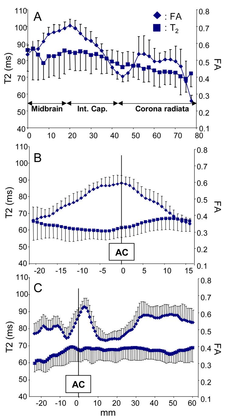
Tract-specific profiles of FA and T2 of the CST (a), the ATR (b), and IFO (c). Abbreviations are; Int. Cap.: internal capsule and AC: anterior commissure. Tract lengths from individual subjects were normalized based on more than 3 anatomical landmarks along their path.

Discussion

Importance of protocol setup and measurement of reproducibility

Tractography is a unique tool that allows us to study white matter architecture three-dimensionally and non-invasively. It can quantitatively illustrate trajectories of various white matter tracts, which is useful not only for educational purposes, but also for advancing our understanding of abnormal brain anatomy. It has been also shown that tractography can be used for quantification studies. Once three-dimensional coordinates of a specific tract are identified, such coordinates can be superimposed on various MR parameter maps to quantify them. However, there are always two important questions that have been repeatedly asked. These are; 1) Precision: how reproducible the results are and 2) Accuracy: how real or valid the results are.

There are no general answers to these questions because they depend on the particular tracts of interest, imaging parameters, and tracking algorithms including choice of ROIs and thresholds for FA and angle). Furthermore, accuracy is not easy to measure because of the lack of a gold standard. On the other hand, with a given tract and reconstruction protocol, it is possible to measure its precision by repeating the measurement. Variability in reconstruction results stem from data acquisition (e.g. SNR, partial volume effect, patient motion, etc) and ROI placement for tracking. The former factors depend on imaging protocols and there are previous publications examining their impacts on the reconstruction results (Heiervang et al., 2006; Huang et al., 2004). The latter can be improved by refining ROI drawing protocols.

This precision (reproducibility) measurement could be one of the most important steps to establish the tractography as a useful research and clinical tool. Even if its accuracy is unknown, if tractography can detect reproducible difference in a specific tract between two groups, this would be an important information to understand disease status or even mechanism.

As for accuracy of tracking results, we reconstructed tracts that are well documented in previous anatomical studies using anatomical constraints (multiple ROIs) based on a priori knowledge. The macroscopic configuration of these reconstructed tracts are, thus, likely to reflect true fiber bundles. However, it is possible that some parts of the trajectory may contain inaccuracy due to partial volume effects, noise, and crossing fibers. It is also important to understand that the visualized pathways do not necessarily reflect brain connectivity because individual axons could be merging and blanching at any points along the bundle. In an extreme case, there may not be any axons that follow the entire path of the reconstructed trajectory.

Setup of reproducible tracking protocols involves two steps. First we need to know which tracts can be reconstructed reproducibly and second we have to refine protocols to reconstruct them. The former step depends on the size, curvature, and discreteness of the tracts. The second factor involves iteration of protocol setup and reproducibility measurements. In our study, we initially identified about 20 known fiber tracts and could develop reproducible protocols for 11 of them. There are several important tracts that are not included in this paper such as fornix, stria terminalis, fimbria, anterior commissure, posterior commissure, body of the corpus callosum, superior thalamic radiation, and optic radiation. These fibers are not included because our current protocols have low reproducibility (κ less than 0.6) or we found large deviations among the healthy subjects. For those fibers with narrow, tubular trajectories (fornix, stria terminalis, anterior and posterior commissure), the reason for the poor reproducibility is most likely due to not enough spatial resolution with respect to the diameter. For the optic radiation, the curvature of tracts at the Meyer's loop is too steep to follow with 2.5 mm pixel resolution. The body of the corpus callosum and the superior thalamic radiation can readily be reconstructed but defining a specific protocol to reproducibly identify 2D slices for ROI drawing is challenging. We would like to emphasize that the reproducibility of tractography results shown in Table 1 are high because these protocols went through optimization procedures to improve the reproducibility and, as mentioned above, those with poor reproducibility were rejected through the process. Therefore, these figures should not be considered as an index of the reproducibility of tractography in general. It is also worth noting that given sufficient thought and technical refining as was done for these eleven tracts, many additional tracts could be reproducibly defined by a laboratory.

The protocols introduced in this paper are not the only reproducible protocols and their reproducibility may vary depending on imaging parameters. Therefore, they should be considered as a guideline. Using these protocols, we measured various MR parameters and size of each tract in normal subjects. The results of the normal variations should provide important information to perform power analysis and judge sensitivity to detect abnormalities.

Tract-specific quantification

As previously pointed out, (Kinoshita et al., 2005) we observed a significant amount of standard deviations in tract sizes. Because intra-rater and inter-rater variability or reproducibility of data acquisition are relatively small (Table 1), the large variability in the population study is likely to have originated from individual anatomical variability. Tractography integrates all events along the tract and thus is influenced by many factors. For example, if results indicate a smaller tract size in a subject, it could be due to the smaller size of the entire length of the tract or there could be one region where the tract is narrowed. Other reasons include perturbation of eigenvectors by crossing fibers and lower anisotropy. In other words, tractography is a method that is very sensitive to various anatomical variations along the trajectory, which leads to a large amount of variability among healthy subjects. It is, at this point, not clear if tractography-based measurement of tract volumes could be a sensitive method to detect anatomical abnormalities due to a pathological condition.

Despite of the large standard deviations of the reconstructed tract sizes, tract-specific T₂ and FA measurement results showed characteristic signatures of individual tracts with small standard deviations. The T₂-FA correlation plot of could separate the corticospinal tracts and the corpus callosum from other tracts. The long T₂ of the CST agrees with previous studies (Yagishita et al., 1994). Once the normal signature of each tract is defined in this type of multi-modal plot, it could be a powerful tool to detect abnormalities in a tract-specific manner. In this respect, it could be an interesting effort to add more parameters such as MTR and T₁. For more in-depth analysis of individual tracts, these MR parameters can be examined along its course as previously demonstrated. (Glenn et al., 2003; Pagani et al., 2005; Partridge et al., 2004; Stieltjes et al., 2001; Virta et al., 1999; Wilson et al., 2003; Xue et al., 1999) Some tracts have rather monotonous profile along their trajectories, while others, such as those shown in Fig. 14, show characteristic and reproducible changes in MR parameters. This approach should provide detailed information to detect regional abnormalities.

The choice of “AND” and “CUT” operations depends on purpose of the study. The “AND” operation should be used when one is interested in characterizing the entire tract while “CUT” is suitable if one segment of a tract needs to be measured. Alternatively, the tract projection method (Fig. 16) could be used in which regions inside and outside the ROIs are spatially separated in the plot.

In Table 2, results of power analyses are tabulated based on our measurement of tract volumes and FA values of normal subjects. This could be used as a quick reference to estimate the number of subjects required to detect abnormalities. While this paper describes reproducibility of tractography procedures and variability in the normal population, we have not characterized image acquisition reproducibility, which is typically measured by scanning the same subject repeatedly. This is obviously a function of signal-to-noise ratio and thus directly related to imaging parameters such as scanning time and image resolution. A comprehensive study to evaluate the image acquisition reproducibility is currently being performed under the initiative of NIH/NCRR-funded Biomedical Informatics Research Network (BIRN, www.nbirn.net) (Farrell et al., 2006).

Table 2.

Power analysis to detect 10, 20, and 40 % changes with p = 0.05 and the power of 0.8.

		CGC	CGH	CST	ATR	SLF	SLFt	ILF	IFO	UNC	Fmaj	Fmin
10%	Volume	518*	337	360	525	342	813	670	298	1354	872	172
	FA	14	12	6	8	11	11	11	12	29	12	4
20%	Volume	126	87	93	130	96	213	173	77	341	220	46
	FA	6	6	4	4	4	4	4	4	10	4	4
40%	Volume	34	55	27	36	27	58	47	27	85	58	12
	FA	4	4	4	4	4	4	4	4	6	4	4

^*The number of subjects required to detect the specified change (averaged values for the right and the left hemisphere). The reported numbers were obtained from DTI datasets with 12 min scanning time.

Numbers may vary depending on SNR and quality of datasets

Asymmetry of tracking results

The finding of asymmetry in the size of fibers in the temporal lobe (SLF, UNC, ILF, and CG) is somewhat unexpected. At this point, we can't conclude which temporal regions account for this difference and whether the difference is caused by difference in anisotropy or actual size of these tracts. Although FA of each tract defined by tractography has low asymmetry, we can not immediately conclude that difference in FA is not the reason for the tract size asymmetry because tractography uses FA as a threshold; difference in FA may manifest as smaller tract size and not necessarily as low FA of the reconstructed tracts. We would like to see if our findings are reproducible in other sites. In this respect, it is noteworthy that the asymmetry of the cingulum (Gong et al., 2005a; Gong et al., 2005b) and the superior longitudinal fasciculus (Makris et al., 2005; Nucifora et al., 2005) has been reported in multiple publications. Park et al performed voxel-based analysis and reported higher FA of the cingulum bundle in the left hemisphere, but otherwise for the uncinate fasciculus. (Park et al., 2004)

Conclusions

Protocols to reconstruct 11 major white matter tracts are described. For these selected white matter tracts, high reproducibility was observed. The established protocols were then applied to a DTI database of adult normal subjects to study size, FA, and T₂ of individual white matter tracts, which revealed characteristic signatures of each tract. Asymmetry of tract size is observed for tracts projecting to the temporal lobe. Our protocol could be used as guidance for tractography-based tract-specific quantification.