

Abstract
The large number of available HIV-1 protease structures provides a remarkable sampling of conformations of the different conformational states, which can be viewed as direct structural information about its dynamics. After structure matching, we apply principal component analysis (PCA) to obtain the important apparent motions, including bound and unbound structures. There are significant similarities between the first few key motions and the first few low-frequency normal modes calculated from a static representative structure with an elastic network model (ENM), strongly suggesting that the variations among the observed structures and the corresponding conformational changes are facilitated by the low-frequency, global motions intrinsic to the structure. Similarities are also found when the approach is applied to an NMR ensemble, as well as to molecular dynamics (MD) trajectories. Thus, a sufficiently large number of experimental structures can directly provide important information about protein dynamics, but ENM can also provide similar sampling of conformations.
Introduction
The Protein Data Bank (Berman et al., 2000) continues to grow rapidly - as of November 2007, over 43,000 protein structures have been deposited there. Among them, many proteins have multiple X-ray structures determined under different conditions. The static X-ray structures may not directly reflect the dynamics of proteins, but they certainly must provide snapshots of the potential motions of proteins. Thus, identifying essential motions by the analysis of multiple structures of the same protein may reveal key information about its dynamics. In addition there are many structures that have been determined by NMR spectroscopy. The conformational ensembles reported for NMR structures also contain multiple conformers which can reveal aspects of protein dynamics. Molecular dynamics (MD) (Rahman, 1964; Stillinger and Rahman, 1974; McCammon et al., 1977) has long been a source for sampling the multiple conformations for the same protein. Through the use of a force field that approximates the atomic interactions within a given protein (and with solvent), MD calculations can yield information about the time-dependent behavior of the molecular system and provide detailed information on the atomic positional fluctuations. At present, MD is widely used for modeling various issues such as ligand binding and protein folding. A MD simulation can generate a large set of conformations starting from a single protein structure, which enables one to study protein motions when only a limited number of structures (or a single structure) is available.
In general, these datasets of multiple structures display conformational changes in high-dimensional spaces, reflecting the cooperativity present in the structures. However, the large numbers of atoms and the complexity of the motions mean that dimensionality reduction is required to comprehend the key motions. One common approach is principal component analysis (PCA) (Pearson, 1901; Hotelling, 1933; Manly, 1986), a statistical method based on covariance analysis. PCA can transform the original space of correlated variables into a reduced space of independent variables (i.e., principal components or PCs). By performing PCA, most of a system’s variance will usually be captured by a small subset of the PCs. PCA has been applied frequently to analyze trajectory data from MD simulations to find the essential dynamics (Amadei et al., 1993, 1996). Recently, Teodoro et al. (Teodoro et al., 2002; 2003) applied PCA to the dataset composed of many conformations for the same protein (HIV-1 protease). They found that PCA can transform the original high-dimensional representation of protein motions into a low-dimensional one that captures the dominant modes of the protein motions. For a typical protein, the system’s dimensionality is thereby reduced from tens of thousands to fewer than fifty degrees of freedom. Howe (Howe, 2001) used PCA to classify the structures in NMR ensemble automatically, according to the correlated structural variations, and the results have shown that the two different representations of the protein structure, the Cα coordinate matrix and the Cα-Cα distance matrix, gave equivalent results and permitted identifying structural differences between conformations.
An alternative method for studying protein motions is normal mode analysis (NMA) (Brooks and Karplus, 1985; Brooks et al., 1988; Case, 1994), in which the concerted motions of a protein are expressed in terms of a set of collective variables (normal modes). Based on Tirion’s (1996) pioneering studies who adopted a single-parameter Hookean potential between nearby atoms for describing protein motions, elastic network models (ENMs) have been extended to coarse-grained models with a simplified single-parameter harmonic potential for modeling (Bahar et al., 1997; Atilgan et al., 2001). The isotropic ENM - Gaussian network model (GNM) (Haliloglu et al., 1997), was developed by Bahar et al. (Bahar et al., 1997). This model applied to coarse-grained proteins having one point mass per residue shows significant agreement with experimental crystallographic B-factors for many proteins. Atilgan et al. (Atilgan et al., 2001) extended the model to include the directions of motions with the anisotropic network model (ANM) (Atilgan et al., 2001).
ENMs can yield a quite large number of modes (n-1 for GNM and 3n-6 for ANM, where n is the number of points or residues for a coarse-grained protein). Since analyzing all modes in detail is unrealistic, especially for large proteins, it is always useful to identify a few key modes for protein motions. Recently, Krebs et al. (Krebs et al., 2002) performed NMA of macromolecular motions and found that most of 3,814 known protein motions can be described well along the directions of a few low-frequency normal modes. In most cases, only one or two low-frequency normal modes are sufficient to capture the major protein motions. Tama et al. (Tama and Sanejouand, 2001) carried out NMA on a dataset containing 20 proteins, each of which has two conformations in “open” and “closed” forms. They compared the overlap between the conformational change (i.e., the displacement vectors between the “open” and “closed” forms) and the normal modes for each given protein, and found that for most proteins, there exists a single low-frequency normal mode that displays a significantly large overlap with the conformational change. Moreover, compared with the experimental conformational change, the overlap values are higher for the normal modes obtained from the “open” form than from the “closed” form. Leo-Macias et al. (2005) conducted an analysis of core deformations in protein superfamilies. They applied PCA to a set of 35 representative protein families and extracted the main deformation modes. They then computed the normal modes using the protein that is the closest to the center of protein family after structural alignments. They found a significant correlation between the deformation modes by PCA and about 20 low-frequency normal modes. These findings suggested that it is possible to identify the key motions that are related to the functions of a protein from analyzing multiple structures of the same protein.
Here we present an approach that can be applied to find the essential protein motions from multiple structures of the same protein, in contrast to using just the two “open” and “closed” conformations in Krebs et al.’s and Tama et al.’s studies. To demonstrate our approach, we use HIV-1 protease for the application, an enzyme that plays a critical role in the life cycle of HIV (Jenwitheesuk and Samudrala, 2003), since there are abundant experimentally determined structures, and the size of the protein is relatively small. The HIV-1 protease functions as a homodimer with a single active site and has three domains: the terminal domain (residues 1–4 and 95–99 of each chain), which is important for the dimerization and stabilization of an active HIV-1 protease; the core domain (residues 10–32 and 63–85 of each chain), which is useful for dimer stabilization and catalytic site stability; and the flap domain, which includes two solvent accessible loops (residues 33–43 of each chain) followed by two flexible flaps (residues 44–62 of each chain), and is important for ligand binding interactions. The conserved Asp25-Thr26-Gly27 active site triad is located at the interface between parts of the core domains. The active site of HIV-1 protease is formed by the homodimer interface and capped by the two flexible flaps. A large conformational change occurs during the process of ligand binding consisting of the opening and closing of the flaps over its binding site. Such principal motions were identified by applying PCA to multiple HIV-1 protease structures, including a set of about 150 crystal structures and a set of conformations generated by MD simulation (Teodoro et al., 2002; 2003). Many computational studies of the motions of this protein have been carried out. Zoete et al. (Zoete et al., 2002) performed MD and NMA studies on a dataset containing 73 X-ray structures of HIV-1 protease inhibitor complexes. They found that the backbone RMSD differences of these X-ray structures showed the same variation as those obtained from MD, NMA and reflected in the X-ray B-factors. They also found that inter-domain motions observed from the X-ray dataset agree with those from MD and NMA. These results suggested that the observed structural fluctuations may be used for measuring the intrinsic protein flexibility. Kurt et al. (Kurt et al., 2003) studied the dynamics of HIV-1 protease by using GNM on observed X-ray structures and MD simulated snapshots. They found that the GNM mode motions from different conformations of the HIV-1 protease are conserved along the MD simulations. The conservation of overall dynamic behavior supports the applicability of GNM for protein motion studies. Chen and Bahar (2004) utilized the GNM (a scalar ENM) motions to identify the most conserved residues within three sub-families of proteases.
In the present study, essential motions are first identified by PCA from a large set of X-ray structures of HIV-1 protease, from an NMR ensemble, and from a conformational ensemble generated from an MD simulation. Next, we calculate the normal modes from elastic network model (ENM) using a representative structure closest to the center of each dataset. Significant similarities are found between these essential motions for all three datasets and the low-frequency normal modes calculated from ENM, strongly suggesting that the dynamics encoded in these datasets is facilitated by the low-frequency, global motions that are intrinsic to the structure. ENM thus provides a coarse-grained, structure-based explanation for the experimentally observed conformational changes upon inhibitor binding or the conformational changes found through MD simulations.
Methods
Datasets
X-ray Structure Dataset I (X-ray-I)
The X-ray structures of the HIV-1 protease were downloaded from the Protein Data Bank (Berman et al., 2000). Those structures with missing residues are excluded, and the remaining 164 structures form our X-ray dataset. We adopt a coarse-grained simplification in which each Cα atom is used to represent its corresponding residue. The representative structure is chosen after aligning all the structures to a reference structure. For the alignment, it matters little which structures are used as the beginning structures since these structures are all quite similar to one another. Since averaging would result in physically unrealistic structures, we use the structure that is the nearest to the average, in this case the PDB 1ebw structure is taken to be the reference structure for subsequent normal mode calculations and MD simulations. The use of slightly different structures for normal mode calculation has little effect upon the results (data not shown). That is due to the insensitivity of the ENM calculations to structural details.
X-ray Structure Dataset II (X-ray-II)
As will become clear from the initial analysis of X-ray structures, there are eight X-ray structures, namely 1b6l, 1b6m, 1b6p, 1mtr, 1rq9, 1rv7, 1rpi, and 1aid, which are significantly different from the remainder of the X-ray structures and represent outliers for the PCA. We therefore create a separate slightly smaller dataset named X-ray-II that is a subset of X-ray-I dataset, by excluding these eight outliers. This modified dataset thus contains 164 − 8 = 156 structures. The reference structure is chosen using the same procedure as for the X-ray-I dataset, and it actually leads to the same structure (PDB code: 1ebw) as for the X-ray-I dataset.
NMR Structures
One PDB file 1bve including 28 structures of the HIV-1 protease is obtained from the Protein Data Bank (Berman et al., 2000). Similarly as for the X-ray case, these NMR structures are aligned and averaged. The structure nearest the average (Number 19 in the ensemble) is used as the reference structure for the normal mode calculation.
MD Structures
The initial structure for the MD simulation is taken to be same as the reference structure (1ebw) of the X-ray dataset. The simulation was performed with the NAMD2 program (Kalé et al., 1999) using the CHARMM27 force field (MacKerell et al., 1998). The simulation was carried out in a TIP3 water box using periodic boundary conditions. Electrostatic interactions were treated with a particle mesh Ewald integration (Darden et al., 1993; Cheatham III et al., 1995). After 100 ps of initial equilibration, the simulation was continued for 10 ns at 300 K and 10,000 structures are collected from the MD trajectory. The structure near the middle of the trajectory is found to be closest to the average of the 10,000 structures (Number 1,583 along the trajectory) is chosen as the reference structure for normal mode calculation.
Principal Component Analysis (PCA)
PCA is performed on the X-ray, NMR and MD datasets respectively. The input is an n by p coordinate matrix X where n is the number of structures and p is 3 times the number of residues (Teodoro et al., 2002; 2003). Each row in X represents the Cα coordinates of each structure. From X the elements of the covariance matrix C are calculated as
| (1) |
where averages over the n structures are indicated by the brackets 〈〉. The covariance matrix C can be decomposed as
| (2) |
where the eigenvectors P represent the principal components (PCs) and the eigenvalues are the elements of the diagonal matrix Δ. The eigenvalues are sorted in descending order. Each eigenvalue is directly proportional to the variance it captures in its corresponding PC.
Anisotropic Network Model (ANM)
ANM is used to calculate the normal modes on the reference structures for the X-ray, NMR and MD datasets. In ANM, the potential energy V is a function of the displacement vector D
| (3) |
where γ is the force constant for all spring interactions of residues (here we used a cutoff distance of 13 Å to establish the spring connections between residues), and H is the Hessian matrix containing the second derivatives of the energy function, which is assumed to be harmonic. For a structure with n residues, the Hessian matrix H contains n × n super-elements of size 3 × 3. The ijth super-elements of H is given as
| (4) |
where Xi, Yi, and Zi are the positional components of residue i, and V represents the harmonic potential between residues i and j, given that residues i and j are in contact and that there is a Hookean spring connecting them. Thus, V can be expressed as
| (5) |
where S0ij is the equilibrium distance between residues i and j, and γ is the spring constant (Atilgan et al., 2001). The Hessian matrix H can be decomposed as
| (6) |
where Λ is a diagonal matrix of the eigenvalues and the eigenvectors form the columns of the matrix M. This decomposition generates 3n-6 normal modes (the first 6 modes account for the rigid body translations and rotations of the system) reflecting the vibrational fluctuations. The eigenvalues are sorted in descending order. Each eigenvalue represents the importance as well as the frequency of the corresponding mode, while the corresponding eigenvector represents the directions and relative magnitudes of the motions of residues.
Overlaps between PCs and Normal Modes
The alignment between the directions of a given PC and a given normal mode is measured by their overlap, which was defined by Tama and Sanejouand (2001)
| (7) |
where Pi is the ith PC and Mj is the jth normal mode. A perfect match yields an overlap value of 1. We define the cumulative overlap (CO) between the first k normal modes and a given PC i as
| (8) |
which measures how well the first k modes together can capture the motion of a single PC.
Relating the PC and Mode Spaces
The overlap between the motion spaces of the first I PCs and the first J low-frequency modes is defined by the root mean-square inner product (RMSIP) (Amadei et al., 1999; Leo-Macias et al., 2005) as
| (9) |
where Pi is the ith PC and Mj is the jth normal mode. This RMSIP indicates how well the motion space spanned by the first I PCs is represented by the first J modes.
Results and Discussion
The RMSD Distribution in the Three Datasets
The initial X-ray dataset (X-ray-I) contains 164 X-ray structures. The RMSD with respect to the reference structure is shown in Figure 2A. There are 4 structures 1b6l, 1b6m, 1b6p and 1mtr that are especially close to each other (RMSD < 0.22 Å), but quite far from the reference structure (RMSD > 3.31 Å). These 4 structures are complexes bound to macrocyclic peptidomimetic inhibitors. Three structures 1rq9, 1rv7 and 1rpi are close to each other (RMSD < 0.58 Å), but far from the reference structure (RMSD > 1.98 Å). These 3 structures are multidrug-resistant HIV-1 proteases. The structure 1aid is 1.40 Å from the reference structure, and is 1.38 Å and 3.81 Å from the average of the groups (1b6l, 1b6m, 1b6p and 1mtr) and (1rq9, 1rv7 and 1rpi), respectively. The aforementioned eight structures, which are the same ones we have excluded by defining the X-ray-II dataset, appear to be quite different from the rest of the structures in their RMS distances to the reference structure. However, the reason why they are considered to be outliers is more evident from the PCA scatter plot analysis in the next section. The structural differences between these outliers and the rest are likely due to the different ligands they bind, the mutational differences or the experimental conditions, etc. For instance, the first group (1b6l, 1b6m, 1b6p and 1mtr) all have a macrocyclic or cyclic inhibitor bound to the enzyme, while the 3 structures in the second group (1rq9, 1rv7 and 1rpi) are multidrug-resistant mutants, each having an expanded active-site cavity. The NMR dataset is an ensemble with 28 conformations. The RMSD with respect to the reference structure is shown in Figure 2B. MD is carried out using NAMD2 and 10,000 structures are obtained from the MD trajectory. The RMSD of each conformation with respect to the starting structure for the MD simulations is shown in Figure 2C. The RMSD with respect to the reference structure is shown in Figure 2D. So, immediately it can be seen that each of our datasets includes a range of conformations having rather similar extents of deviations from their characteristic conformation.
Figure 2.

RMSD with respect to the reference structure for: (A) X-ray-I dataset, with the RMSD values sorted in ascending order. X-ray-II dataset is the same as X-ray-I, excluding the eight structures that have significantly larger RMSD values than the rest. (B) NMR dataset, sorted by the RMSD values in ascending order. (C) MD dataset, shown in the order of the time steps along the 10 ns simulation. (D) MD dataset, sorted by the RMSD values in ascending order.
Dimensionality Reduction by PCA
PCA is performed on the X-ray datasets. The fraction of variance and the cumulative fraction of variance explained by the first 6 PCs are shown in Figure 3A and 3B. It can be seen that the first 2 PCs explain 50% and 16% of the variance respectively and the first 6 PCs together explain over 85% of the variance for X-ray-I dataset. For X-ray-II dataset, the first 2 PCs explain 28% and 15% of the variance respectively and the first 6 PCs together explain over 67%. PCA is also performed on the 28 NMR structures. The fraction of variance and the cumulative fraction of variance explained by the first 6 PCs are shown in Figure 3C. It can be seen that the first 2 PCs explain 38% and 23% of the variance respectively. The first 6 PCs together explain over 79% of the variance. Lastly, PCA is performed on the MD simulated structures. From the fraction of variance and the cumulative fraction of variance plots (Figure 3D), it can be seen that the first 2 PCs explain 22% and 10% of the variance respectively, and the first 6 PCs together account for about 55% of the variance. The above results indicate that most of the internal motions of the protein can be captured by only a few principal motions (the first several PCs). It is also noted that the first 6 PCs capture variance better for X-ray and NMR structures than for the MD structures.
Figure 3.

The fraction of variance (‘o’) and the cumulative fraction of variance (‘x’) represented by the first 6 PCs for: (A) X-ray-I dataset. (B) X-ray-II dataset. (C) NMR dataset. (D) MD dataset.
PCA Scatter Plots
The PCA scores can provide a simple overview of all the structures in the dataset. Scatter plots of two PCA scores show the distribution of the actual structure's deviations from the characteristic structure plotted along the directions of these two PCs. An ideal representation by the PCs will have the structures quite uniformly distributed about the center of these plots. For the X-ray-I dataset, the scatter plot of PC 1 and PC 2 (Figure 4A) shows that most structures are close to the reference structure and are clustered into one group. The classified small groups (1b6l, 1b6m, 1b6p, 1mtr), (1rq9, 1rv7, 1rpi) and 1aid appear as outliers, which is consistent with their RMSD distributions seen earlier. The scatter plot of PC 1 and PC 3 (Figure 4B) further confirms the above classification. The scatter plots for the X-ray-II dataset, after excluding the outliers are shown in Figures 4C and 4D. In the NMR case, the scatter plot of PC 1 and PC 2 (Figure 4E) and the scatter plot of PC 1 and PC 3 (Figure 4F) show the 28 structures distributed along the 2-PC projection. In the MD case, the scatter plot of PC 1 and PC 2 (Figure 4G) and the scatter plot of PC 1 and PC 3 (Figure 4H) show the 10,000 structures (represented by 100 data points) distributed along the 2-PC projection. It is seen that the results from the unpruned X-ray dataset (X-ray-I) are characteristically different from the others, which are more comparable to one another. The first two PCs of the unpruned X-ray dataset mainly reflect the characteristics of those eight outliers whose large RMS deviations enable them to dominate the rest of X-ray structures in influencing the directions of the first two PCs. Therefore, it has been necessary to exclude these and to form a separate dataset X-ray-II in order to identify the key motions of the remaining 156 X-ray structures. Unless otherwise specified, X-ray-II is the dataset we will use for the X-ray structures henceforth.
Figure 4.

Distribution of individual structures along pairs of the first three principal component directions. Shown are the planes of PC 1 and PC 2 and of PC 1 and PC 3 for X-ray-I, X-ray-II, NMR and MD datasets respectively. (For the MD dataset, the 10,000 data points are represented by 100 data points by coarse-graining.)
Identification and Visualization of the Principal Motions
Because most of the protein displacements, in terms of the variance of the structures, can be captured by only a first few principal components (PCs), these PCs can thus be used to characterize the dominant dynamical behaviors of the protein. The X-ray dataset is direct experimental evidence (snapshots) of protein dynamics. PCA enables us to analyze these experimental data and identify a few key directions of motions, i.e., those along the first few PCs. Note that most X-ray structures of HIV-1 protease have some drug molecules bound and thus their conformational displacements reflect the effects of such ligand binding. Therefore, the key directions of motions identified after applying PCA to the X-ray data may provide valuable insights for drug design, such as what the available conformational subspace is, the geometry variance of the binding site, the accessibility of the binding site and the potential pathways for a candidate ligand to reach it (Singh et al., 1999; Bayazit et al., 2000).
Figure 5 shows the residue fluctuations of the first 3 principal motions (the first 3 PCs) of each dataset. As mentioned earlier, the first 2 PCs of the original X-ray dataset (X-ray-I) mainly reflect the deviations of the eight outliers (namely 1b6l, 1b6m, 1b6p, 1mtr, 1rq9, 1rv7, 1rpi, and 1aid) and their distinct features of motions. For the PC 1 motion, the second half of each protein chain has significantly larger amplitudes of fluctuations than the first half and is nearly symmetric for the two chains that form the dimer. Since structures 1b6l, 1b6m, 1b6p, and 1mtr have a dominant PC 1 component (see Figure 4A and 4B), the PC 1 motion mainly reflects their “motions” (or deviations) relative to the reference structure. For the PC 2 motion, there are large amplitudes of fluctuations at the two flaps and is again nearly symmetric for the two chains, which is a feature distinguishing structures 1rq9, 1rv7, 1rpi, and 1aid from the rest. The symmetry between the two chains of this homodimer, however, is much less obvious, sometimes even hardly visible, in the PC 1 and PC 2 fluctuation plots (and higher PCs as well) for the other datasets such as X-ray-II dataset (see Figure 5 (X-ray-II)), where the amplitudes of the conformational displacements are much smaller. The decreased data/noise ratio is the main reason for the apparent loss of symmetry. Visualization of the first dominant motion direction (PC 1) of X-ray-II is shown in Figure 6A together with that of the ENM mode that closely resembles it (see Figure 6B).
Figure 5.

Residue positional fluctuations of the first 3 PCs in each dataset. Note that the PC 1 and PC 2 in the X-ray-I dataset have symmetrical fluctuations for the two protein chains (the first chain: residues 1–99; the second chain: residues 100–198). But no symmetrical fluctuations are observed for the X-ray-II, NMR and MD datasets.
Figure 6.
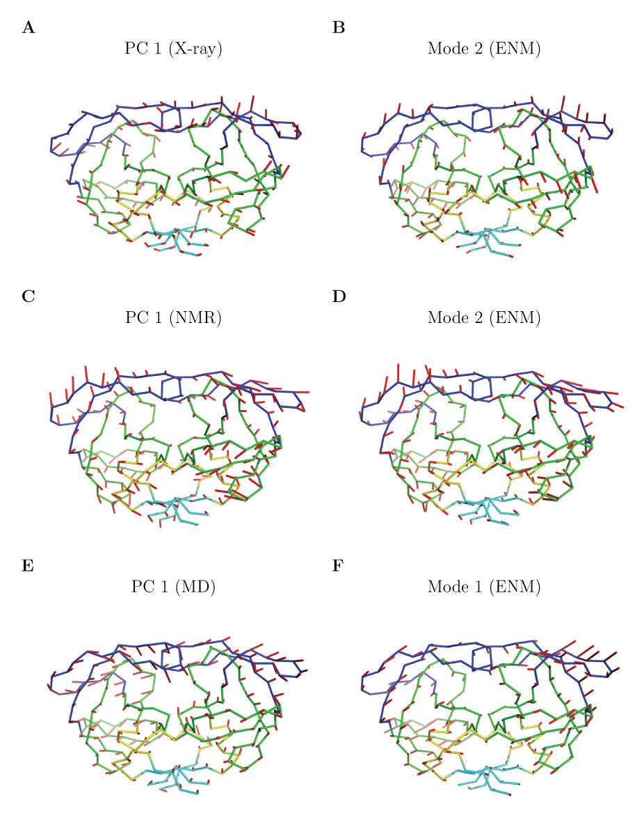
Visualizations of the motions of the dominant PCs (left column) and the most similar corresponding modes predicted by ENM (right column). In the X-ray-II dataset, the overlap between (A) PC 1 and (B) Mode 2 is 0.52. In the NMR dataset, the overlap between (C) PC 1 and (D) Mode 2 is 0.91. In the MD dataset, the overlap between (E) PC 1 and (F) Mode 1 is 0.74. Blue - the flap domain; green - the core domain; cyan - the terminal domain; yellow - other residues. The motions of PCs and modes are shown as red sticks with the directions indicated. The stick lengths represent the relative amplitudes of fluctuations of the corresponding residue.
Similarly, PCA is also applied to the NMR ensemble and the MD dataset to identify the key motions. An NMR ensemble can be more advantageous than a single X-ray structure in that it provides more than the mean-square fluctuations of each atom, but also may provide some directional information on protein dynamics. In our case, the NMR ensemble for HIV-1 protease (PDB code: 1bve) includes 28 conformers. A few key directions of motion are revealed and visualized (see Figure 6C for PC 1), which may represent the dominant motion directions of the protein in solution. Interestingly, the direction of PC 1 aligns extremely well with one mode predicted by ENM, which is shown in Figure 6D. PCA applied to the MD dataset (10,000 structures) reveals the dominant motions of the protein in simulation (see Figure 6E for the visualization of PC 1 of MD dataset). One advantage of MD is that it can easily be used to generate many structures by computer simulation, but on the other hand to its disadvantage it is difficult to know how well the conformational space is represented or how biased the data may be. However, we also see significant matches between the dominant directions identified by PCA and those calculated from ENM (see Figure 6E and 6F and more in the next section).
It is noted that the fluctuation profiles of the first several PCs are quite different between the datasets (X-ray, NMR and MD), see Figure 5. Such differences in the fluctuation profiles reflect the difference in dynamics among the datasets. The principal component axes in one dataset may not perfectly align with those in another dataset. For instance, it is not expected that the PC 1 of an X-ray dataset would match perfectly with the PC 1 in the NMR dataset, but rather it may be expressed as a combination of a few PCs of the NMR dataset. Yet, as will be seen later, these distinct PC profiles can all be described by a set of low-frequency ENM modes. As shown in Table 1C, the subspace of the first several PCs can be well captured by the first several low-frequency ENM modes for all the datasets. This is quite remarkable, and it suggests that the ENM normal modes have captured well the essential motions found in all datasets, although there are some differences in dynamics encoded in the different datasets.
Table 1.
(A) Overlaps between the first 3 PCs and the first 3 low-frequency normal modes. The bold values are the largest values for each dataset. (B) The cumulative overlap (CO) between the first 3 PCs and a set of low-frequency normal modes. (C) The RMSIP between the PC and mode spaces.
| (A) | X-ray-II | NMR | MD | ||||||
|---|---|---|---|---|---|---|---|---|---|
| PC 1 | PC 2 | PC 3 | PC 1 | PC 2 | PC 3 | PC 1 | PC 2 | PC 3 | |
| Mode 1 | 0.46 | 0.27 | 0.24 | 0.25 | 0.88 | 0.02 | 0.74 | 0.03 | 0.12 |
| Mode 2 | 0.52 | 0.31 | 0.20 | 0.91 | 0.28 | 0.05 | 0.23 | 0.26 | 0.28 |
| Mode 3 | 0.17 | 0.51 | 0.31 | 0.02 | 0.04 | 0.30 | 0.16 | 0.14 | 0.65 |
| (A) Overlap between a single PC and one mode | |||||||||
| (B) | X-ray-II | NMR | MD | ||||||
|---|---|---|---|---|---|---|---|---|---|
| PC 1 | PC 2 | PC 3 | PC 1 | PC 2 | PC 3 | PC 1 | PC 2 | PC 3 | |
| 3 modes | 0.71 | 0.66 | 0.43 | 0.94 | 0.92 | 0.31 | 0.79 | 0.30 | 0.72 |
| 6 modes | 0.74 | 0.68 | 0.48 | 0.95 | 0.94 | 0.35 | 0.82 | 0.49 | 0.77 |
| 20 modes | 0.84 | 0.73 | 0.62 | 0.96 | 0.95 | 0.46 | 0.89 | 0.67 | 0.83 |
| (B) Overlap between one PC and a set of modes | |||||||||
| (C) | X-ray-II | NMR | MD | |||
|---|---|---|---|---|---|---|
| 3 PCs | 6 PCs | 3 PCs | 6 PCs | 3 PCs | 6 PCs | |
| 3 modes | 0.61 | 0.53 | 0.78 | 0.61 | 0.64 | 0.59 |
| 6 modes | 0.65 | 0.57 | 0.80 | 0.66 | 0.71 | 0.70 |
| 20 modes | 0.74 | 0.68 | 0.83 | 0.74 | 0.80 | 0.81 |
| (C) Overlap between PC and mode subspaces | ||||||
Large Overlaps between PCs and Normal Modes - A Structure-Based Explanation of Observed Motions
The dominant directions of motions represented by the first few PCs have been obtained by direct principal component analysis (PCA) of experimental data (X-ray or NMR) and MD trajectories. In this section, we will investigate whether there are structure-based and physics-based explanations for these directions of motions. In other words, are there intrinsic reasons why these directions of motions are preferred?
For this purpose, we compare these directions of motions with the computationally predicted mode motions by ENM. We calculate the overlaps between the first few PCs and low-frequency modes according to Eq. 5, for the 3 datasets. In all the cases, we observe some large overlap values between the first several PCs and a few low-frequency modes. The results imply that the observed structures and the corresponding conformational changes are likely facilitated by the low-frequency, global motions that are intrinsic to the structure. ENM thus provides a coarse-grained, structure-based explanation for the experimentally observed conformational changes taking place mostly upon inhibitor binding (for the X-ray structures), as well as for the dynamics revealed from both the NMR ensemble and the simulated MD dataset.
In addition to providing a structure-based explanation for the experimentally observed conformational changes, the mode motions of the protein from ENM can also be used to predict the collective motions of the protein that have not been detected in crystal or NMR structures. Further, when combined with the experimentally observed conformational changes, they can deepen our understanding of the dynamics of the protein, and provide specific information regarding the dynamics in the vicinity of the binding site, e.g., the motion of the flaps. Such an understanding (and visualization) of the dynamics may provide key insights for better ways to design new drugs for protein targets.
Matching a Single PC with a Single Mode
The overlaps between the first 3 PCs and the first 3 low-frequency modes (Mode 1–3) are shown in Table 1A. In the X-ray-II dataset, the largest overlap is 0.52, between PC 1 and Mode 2. The overlap between PC 2 and Mode 3 is 0.51. In the NMR dataset, the largest overlap is 0.91, between PC 1 and Mode 2. The overlap between PC 2 and Mode 1 is 0.88. In the MD dataset, the largest overlap is 0.74, between PC 1 and Mode 1. The overlap between PC 3 and Mode 3 is 0.65. These results indicate that the principal motions (i.e., the first few PCs) can be explained well by a single low-frequency normal mode in each of the X-ray, NMR and MD cases.
The largest overlaps found for the first two PCs of the NMR ensemble are highly significant, at 0.91 and 0.88 respectively (see Table 1A). This significance has two implications. On one hand, as mentioned above, the dynamics revealed from applying PCA to the NMR ensemble yields a structure-based explanation. On the other hand, the NMR ensembles promise improved agreements over the X-ray structures, so that the dynamics revealed may provide an important validation tool of the accuracy of the ENM modes of motion. The large overlaps suggest that the ENM, even though coarse-grained, can capture well the essential dynamics of protein in solution (for the NMR case). In a recent study by Yang et al. (2007), they applied GNM to both X-ray structures and NMR ensembles of the same proteins, and find GNM is able to reproduce the residue fluctuations in NMR structures better than that from X-ray structures. These results also support the applicability of ENM to capture the dynamics of NMR structures.
However, we also see that the larger overlap for the third PC of the NMR dataset is far smaller (0.30). This is mainly because there are only 28 structures in the NMR ensemble, which means that higher PCs may quickly become unreliable. Therefore, a larger ensemble or more ensembles are desired. Unfortunately, there is no other NMR structure available for HIV-1 protease in the Protein Data Bank. A more thorough study using other NMR ensembles of structures is underway.
Principal Motion (PC) Represented by A Few Modes
Since ENM is a coarse-grained model, it is possible that each individual mode may not be so precise. The details of each normal mode will of course depend on the force field details. However, the subspace of the low-frequency modes is much less affected by such details (Hinsen et al., 1999; Song and Jernigan, 2007), and it has been shown that the overall shape is dominant in determining the motions of the slower modes (Doruker and Jernigan, 2003; Lu and Ma, 2005; Ming et al., 2002). Therefore, it is worthwhile to determine how well a given principal motion (PC) can be represented by a few low-frequency normal modes collectively. To do so, we calculate the cumulative overlap (CO) for each PC with the subspace defined by the first few low-frequency normal modes.
The results in Table 1B show that even with 3 modes, overlap values are usually significantly improved. More improvements are gained across the board when the first 20 low-frequency modes are used. The cumulative overlap for PC 3 of the NMR set remains relatively low. As pointed out earlier, this is mainly due to the small size of the NMR ensemble, which renders its high PCs undependable. In summary, the principal motions determined from PCA can be well captured by a small number of low-frequency normal modes.
Overlaps between PC and Mode Subspaces
The first few PCs collectively capture the majority of the total variance. So the subspace spanned by these PCs reflects the dominant motion space of the protein. To measure how well this motion space can be captured by the first several low-frequency normal modes, we calculated the RMSIP (see Eq. 7) between the two spaces. Intuitively, RMSIP measures the percentage of the PC subspace that is covered by the subspace spanned by the selected low-frequency modes.
Table 1C lists the RMSIP values between the subspaces spanned by the first 6 PCs with those spanned by the first 3, 6, and 20 modes. Large RMSIP values are seen even with 3 modes, and marginal improvements are achieved as more modes are included, until the RMSIP values reach about 0.7 (or 70%) when the first 20 low-frequency modes are considered. These results suggest that the majority of the dynamics displayed in these datasets can be explained by a small set of the ENM modes. This, in addition to ENM’s success in interpreting the crystal B-factors of X-ray structures and the NMR ensembles (Yang et. al., 2007), confirms the validity of using ENM to study protein dynamics. And, these include the dynamics from a broad range of cases, that in crystals, in solution, or from MD simulations.
Though ENMs are coarse-grained models, their usefulness in capturing the collective dynamics of macromolecules has been proved over the last decade. Here we can see again in Table 1C that the subspace spanned by the first 20 low-frequency modes of the ENM matches quite well with the subspace spanned by the PCs of the X-ray and the NMR structures, as well as that of the MD trajectory.
Significance Test of Overlap Values
To test whether the large overlaps we have obtained in Table 1A are statistically significant, we have conducted a permutation test. In the following, we carry out a test on the overlap between PC 1 and Mode 2 (0.52) of X-ray-II dataset to demonstrate our approach. In the test, at each iteration, the order of the columns in the coordinate matrix X is permuted randomly. PCA is then performed on the permuted X and the overlap is computed. The simulation is carried out 1,000 times and an empirical distribution of overlaps is generated. This empirical distribution plays the role of the null distribution for hypothesis testing and enables us to estimate the probability of observing an overlap at least as large as the one observed if in fact there were no association between the motion spaces estimated under the two approaches. Based on the simulation, the observed value 0.52 is larger than most of the values obtained from the permuted dataset, corresponding to a p-value below 0.0001.
Conclusions
In this study we have identified the key directions of motion of the HIV-1 protease from crystal structures, in solution, and from MD simulations. This is accomplished by applying PCA to the more than 150 available X-ray structures of the protein, an NMR ensemble (28 models), and the simulated structures generated from a 10 ns MD simulation. These key motions reveal some important dynamic behaviors of the protein and thus should be able to provide valuable new insights for drug design. Moreover, large overlaps between the first few of these key motions (or PCs) and the first few low-frequency normal modes of ENM are seen, suggesting that the observed structures and the corresponding conformational changes are facilitated by the low-frequency, global motions that are intrinsic to the structure. ENM thus provides a coarse-grained, structure-based explanation for the experimentally observed conformational changes. This, in addition to ENM’s success in interpreting the crystal B-factors of X-ray structures, confirms its validity for studying protein dynamics. And the dynamics can be that in crystals, or in solutions, or from simulations. Even though the dynamics encoded in these different datasets are not necessarily fully identical, nonetheless the ENM normal modes have been shown to capture well the essential motions found in all of these datasets (see Table 1C).
Our approach may also help identify which modes contribute most to the functional motions. For example, from the normal mode calculations alone, it cannot be directly established which normal mode is actually the most important one functionally. By using our approach, one may first employ PCA to obtain the principal motions, and then identify the most important normal mode(s) by comparing them with the principal motions - the modes having the largest overlaps being the obvious candidates.
Figure 1.

Cartoon representation (A) and alpha carbon trace (B) of the HIV-1 protease structure. Blue - the flap domain; green - the core domain; cyan - the terminal domain; yellow - other residues. The red spheres represent the conserved Asp25-Thr26-Gly27 active site triad. The figure was created using PyMOL (DeLano Scientific).
Acknowledgment
We would like to thank Dr. Xuefeng Zhao for computer support and valuable iscussion. We gratefully acknowledge the support from NIH Grants GM-072014 and GM-073095, together with NSF Grant CNS-05-515. Dr. Alicia Carriquiry’s work is partially funded by NSF Grant DMS-0502347.
Footnotes
Publisher's Disclaimer: This is a PDF file of an unedited manuscript that has been accepted for publication. As a service to our customers we are providing this early version of the manuscript. The manuscript will undergo copyediting, typesetting, and review of the resulting proof before it is published in its final citable form. Please note that during the production process errors may be discovered which could affect the content, and all legal disclaimers that apply to the journal pertain.
References
- Amadei A, Ceruso MA, Di Nola A. On the convergence of the conformational coordinates basis set obtained by the essential dynamics analysis of proteins ’ molecular dynamics simulations. Proteins. 1999;36:419–424. [PubMed] [Google Scholar]
- Amadei A, Linssen AB, Berendsen HJ. Essential dynamics of proteins. Proteins. 1993;17:412–425. doi: 10.1002/prot.340170408. [DOI] [PubMed] [Google Scholar]
- Amadei A, Linssen AB, de Groot BL, van Aalten DM, Berendsen HJ. An efficient method for sampling the essential subspace of proteins. J. Biomol. Struct. Dyn. 1996;13:615–625. doi: 10.1080/07391102.1996.10508874. [DOI] [PubMed] [Google Scholar]
- Atilgan AR, Durell SR, Jernigan RL, Demirel MC, Keskin O, Bahar I. Anisotropy of fluctuation dynamics of proteins with an elastic network model. Biophys. J. 2001;80:505–515. doi: 10.1016/S0006-3495(01)76033-X. [DOI] [PMC free article] [PubMed] [Google Scholar]
- Bahar I, Atilgan AR, Erman B. Direct evaluation of thermal fluctuations in proteins using a single-parameter harmonic potential. Folding Des. 1997;2:173–181. doi: 10.1016/S1359-0278(97)00024-2. [DOI] [PubMed] [Google Scholar]
- Bayazit OB, Song G, Amato NM. Enhancing randomized motion planners: Exploring with haptic hints; Proc. IEEE Int. Conf. Robot. Autom. (ICRA); 2000. pp. 529–536. [Google Scholar]
- Berman HM, Westbrook J, Feng Z, Gilliland G, Weissig TNBH, Shindyalov IN, Bourne PE. The protein data bank. Nucl. Acids Res. 2000;28:235–242. doi: 10.1093/nar/28.1.235. [DOI] [PMC free article] [PubMed] [Google Scholar]
- Brooks B, Karplus M. Normal modes for specific motions of macromolecules: application to the hinge-bending mode of lysozyme. Proc. Natl. Acad. Sci. USA. 1985;82:4995–4999. doi: 10.1073/pnas.82.15.4995. [DOI] [PMC free article] [PubMed] [Google Scholar]
- Brooks CL, Karplus M, Pettitt BM. Proteins: a theoretical perspective of dynamics, structure, and thermodynamics. Adv. Chem. Phys. 1988;71:1–249. [Google Scholar]
- Case DA. Normal mode analysis of protein dynamics. Curr. Opin. Struct. Biol. 1994;4:285–290. [Google Scholar]
- Cheatham TE, III, Miller JL, Fox T, Darden TA, Kollman PA. Molecular dynamics simulations on solvated biomolecular systems: the particle mesh Ewald method leads to stable trajectories of DNA, RNA, and proteins. J. Amer. Chem. Soc. 1995;117:4193–4194. [Google Scholar]
- Chen S-C, Bahar I. Mining frequent patterns in protein structures: a study of protease families. Bioinformatics. 2004;20 Suppl. 1:i77–i85. doi: 10.1093/bioinformatics/bth912. [DOI] [PMC free article] [PubMed] [Google Scholar]
- Darden TA, York DM, Pedersen LG. Particle mesh Ewald: An N·log(N) method for Ewald sums in large systems. J. Chem. Phys. 1993;98:10089–10092. [Google Scholar]
- Doruker P, Jernigan RL. Functional motions can be extracted from on-lattice construction of protein structures. Proteins. 2003;53:174–181. doi: 10.1002/prot.10486. [DOI] [PubMed] [Google Scholar]
- Haliloglu T, Bahar I, Erman B. Gaussian dynamics of folded proteins. Phys. Rev. Lett. 1997;79:3090–3093. [Google Scholar]
- Hinsen K, Thomas A, Field MJ. Analysis of domain motions in large proteins. Proteins. 1999;34:369–382. [PubMed] [Google Scholar]
- Hotelling H. Analysis of a complex of statistical variables into principal components. J. Educational Psychol. 1933;24:441. [Google Scholar]
- Howe PW. Principal components analysis of protein structure ensembles calculated using NMR data. J. Biomol. NMR. 2001;20:61–70. doi: 10.1023/a:1011210009067. [DOI] [PubMed] [Google Scholar]
- Jenwitheesuk E, Samudrala R. Improved prediction of HIV-1 protease-inhibitor binding energies by molecular dynamics simulations. BMC Structural Biology. 2003;3:2. doi: 10.1186/1472-6807-3-2. [DOI] [PMC free article] [PubMed] [Google Scholar]
- Kalé L, Skeel R, Bhandarkar M, Brunner R, Gursoy A, Krawetz N, Phillips J, Shinozaki A, Varadarajan K, Schulten K. NAMD2: greater scalability for parallel molecular dynamics. J. Comput. Phys. 1999;151:283–312. [Google Scholar]
- Krebs WG, Alexandrov V, Wilson CA, Echols N, Yu H, Gerstein M. Normal mode analysis of macromolecular motions in a database framework: developing mode concentration as a useful classifying statistic. Proteins. 2002;48:682–695. doi: 10.1002/prot.10168. [DOI] [PubMed] [Google Scholar]
- Kurt N, Scott WR, Schiffer CA, Haliloglu T. Cooperative fluctuations of unliganded and substrate-bound HIV-1 protease: a structure-based analysis on a variety of conformations from crystallography and molecular dynamics simulations. Proteins. 2003;51:409–422. doi: 10.1002/prot.10350. [DOI] [PubMed] [Google Scholar]
- Leo-Macias A, Lopez-Romero P, Lupyan D, Zerbino D, Ortiz AR. An analysis of core deformations in protein superfamilies. Biophys. J. 2005;88:1291–1299. doi: 10.1529/biophysj.104.052449. [DOI] [PMC free article] [PubMed] [Google Scholar]
- Lu M, Ma J. The role of shape in determining molecular motions. Biophys. J. 2005;89:2395–2401. doi: 10.1529/biophysj.105.065904. [DOI] [PMC free article] [PubMed] [Google Scholar]
- MacKerell AD, Bashford D, Jr, Bellott M, Dunbrack RL, Evanseck JD, Jr, Field MJ, Fischer S, Gao J, Ha HGS, Joseph-McCarthy D, Kuchnir L, Kuczera K, Lau FTK, Mattos C, Michnick S, Ngo T, Nguyen DT, Prodhom B, Reiher WE, Roux B, III, Schlenkrich M, Smith JC, Stote R, Straub J, Watanabe M, Wiórkiewicz-Kuczera J, Yin D, Karplus M. All-atom empirical potential for molecular modeling and dynamics studiesof proteins. J. Phys. Chem. B. 1998;102:3586–3616. doi: 10.1021/jp973084f. [DOI] [PubMed] [Google Scholar]
- Manly B. Multivariate statistics - A primer. Boca Raton: Chapman & Hall/CRC; 1986. [Google Scholar]
- McCammon JA, Gelin BR, Karplus M. Dynamics of folded proteins. Nature. 1977;267:585–590. doi: 10.1038/267585a0. [DOI] [PubMed] [Google Scholar]
- Ming D, Kong Y, Lambert MA, Huang Z, Ma J. How to describe protein motion without amino acid sequence and atomic coordinates. Proc. Natl. Acad. Sci. USA. 2002;99:8620–8625. doi: 10.1073/pnas.082148899. [DOI] [PMC free article] [PubMed] [Google Scholar]
- Pearson K. On lines and planes of closest fit to systems of points in space. The London, Edinburgh and Dublin Philosophical Magazine and Journal of Science. 1901;2:572. [Google Scholar]
- Rahman A. Correlations in the motion of atoms in liquid argon. Phys. Rev. A. 1964;136:405–411. [Google Scholar]
- Singh AP, Latombe JC, Brutlag DL. A motion planning approach to flexible ligand binding; The 7th Int. Conf. on Intelligent Systems for Molecular Biology (ISMB); 1999. pp. 252–261. [PubMed] [Google Scholar]
- Song G, Jernigan RL. vGNM: a better model for understanding the dynamics of proteins in crystals. J. Mol. Biol. 2007;369:880–893. doi: 10.1016/j.jmb.2007.03.059. [DOI] [PMC free article] [PubMed] [Google Scholar]
- Stillinger FH, Rahman A. Improved simulation of liquid water by molecular dynamics. J. Chem. Phys. 1974;60:1545–1557. [Google Scholar]
- Tama F, Sanejouand YH. Conformational change of proteins arising from normal mode calculations. Protein Eng. 2001;14:1–6. doi: 10.1093/protein/14.1.1. [DOI] [PubMed] [Google Scholar]
- Teodoro ML, Phillips GN, Jr, Kavraki LE. A dimensionality reduction approach to modeling protein flexibility; Int. Conf. Comput. Mole. Biol. (RECOMB); 2002. pp. 299–308. [DOI] [PubMed] [Google Scholar]
- Teodoro ML, Phillips GN, Jr, Kavraki LE. Understanding protein flexibility through dimensionality reduction. J. Comput. Biol. 2003;10:617–634. doi: 10.1089/10665270360688228. [DOI] [PubMed] [Google Scholar]
- Tirion MM. Large amplitude elastic motions in proteins from a single-parameter, atomic analysis. Phys. Rev. Lett. 1996;77:1905–1908. doi: 10.1103/PhysRevLett.77.1905. [DOI] [PubMed] [Google Scholar]
- Yang L, Eyal E, Chennubhotla C, Jee J, Gronenborn AM, Bahar I. Insights into equilibrium dynamics of proteins from comparison of NMR and X-ray data with computational predictions. Structure. 2007;15:741–749. doi: 10.1016/j.str.2007.04.014. [DOI] [PMC free article] [PubMed] [Google Scholar]
- Zoete V, Michielin O, Karplus M. Relation between sequence and structure of HIV-1 protease inhibitor complexes: a model system for the analysis of protein flexibility. J. Mol. Biol. 2002;315:21–52. doi: 10.1006/jmbi.2001.5173. [DOI] [PubMed] [Google Scholar]