Blind separation of auditory event-related brain responses into independent components

Abstract

Averaged event-related potential (ERP) data recorded from the human scalp reveal electroencephalographic (EEG) activity that is reliably time-locked and phase-locked to experimental events. We report here the application of a method based on information theory that decomposes one or more ERPs recorded at multiple scalp sensors into a sum of components with fixed scalp distributions and sparsely activated, maximally independent time courses. Independent component analysis (ICA) decomposes ERP data into a number of components equal to the number of sensors. The derived components have distinct but not necessarily orthogonal scalp projections. Unlike dipole-fitting methods, the algorithm does not model the locations of their generators in the head. Unlike methods that remove second-order correlations, such as principal component analysis (PCA), ICA also minimizes higher-order dependencies. Applied to detected—and undetected—target ERPs from an auditory vigilance experiment, the algorithm derived ten components that decomposed each of the major response peaks into one or more ICA components with relatively simple scalp distributions. Three of these components were active only when the subject detected the targets, three other components only when the target went undetected, and one in both cases. Three additional components accounted for the steady-state brain response to a 39-Hz background click train. Major features of the decomposition proved robust across sessions and changes in sensor number and placement. This method of ERP analysis can be used to compare responses from multiple stimuli, task conditions, and subject states.

Although the locations of the brain areas generating event-related potentials (ERPs) cannot be uniquely determined by scalp recordings from any number of channels (1), several methods have been proposed for decomposing evoked responses into activations of distinct neural sources. Most of these also attempt to locate the active areas, by assuming either that they have a known or simple spatial configuration (2) or that generators are restricted to a small subset of possible locations and orientations (3). Other methods based on rotations of principal components use optimization criteria not directly related to brain anatomy and physiology. These methods may assume that each response component has the same time course of activation in every experimental condition (4). All these methods use second-order spatiotemporal correlations to perform the decomposition.

Here we report a statistical method for decomposing one or more event-related brain responses into a sum of components with spatially fixed scalp distributions and maximally independent (though possibly overlapping) time courses. Independence requires the absence of higher-order as well as second-order correlations between the time courses. Independence, therefore, is a stronger condition than decorrelation and, in particular, is not satisfied by decomposition into principal components by principal component analysis (PCA).

Although the neural mechanisms that generate ERPs are not known, the assumptions underlying the application of the independent component analysis (ICA) algorithm (5) to ERP data are generally compatible with a widely assumed model. Anatomical and physiological studies have shown that sensory perception and processing occur in multiple cortical areas, as revealed in many current brain imaging studies (6). Averaged ERPs evoked by sensory stimuli and recorded from the scalp are thought to be generated in conjunction with synchronous activity in radially oriented pyramidal cells in the activated areas. Because volume conduction through the cerebrospinal fluid, skull, and scalp is thought to be linear, sensory ERPs are assumed to sum brief and relatively spatially stable potentials associated with synchronous activation of neuropil in each stimulated area.

Activity in neuronal fibers connecting cortical areas does not produce macroscopic fields visible from the scalp. Thus the activity underlying sensory evoked responses has a saltatory character; individual features of sensory ERPs index discrete stages within one or more parallel streams of sensory processing, each stage involving potentials generated in one or more cortical areas. However, the scalp distributions of these generators may overlap in time and space, causing the ERP topography to shift continuously and making decomposition into spatially fixed activations difficult. For example, if two fixed dipole-like sources in anterior and posterior cortex were to have spatially overlapping activations with a small delay between them, the scalp potentials they generate would have the appearance of a wave sweeping from front to back on the scalp.

When subjects process sensory signals for their meaning or task relevance, later features appear in the ERP whose spatial scalp patterns are often inconsistent with an origin in sensory cortex. These are believed to index the later cognitive processing of relevant stimulus attributes or information within frontal, inferior, or possibly widespread cortical areas, after this information is first extracted in early sensory areas. A subject’s preexisting level of arousal and attention to the stimuli can also affect the strength of early evoked response components (7).

ICA yields data decompositions consistent with the standard view of ERP genesis outlined above, since the spatially stable and sparsely active components sum to the observed multichannel responses. ICA determines what spatially fixed and temporally independent component activations compose an observed time-varying response, without attempting to directly specify where in the brain these activations arise. Each ICA component is specified by a fixed linear spatial filter that determines a time course of activation during each response condition, plus a fixed pattern of strengths at each of the scalp electrodes. Data from N electrodes can be reconstructed as the sum of the N independent components.

Previously, we showed that the ICA algorithm can be used to separate neural activity from recording and muscle artifacts in spontaneous electroencephalographic (EEG) data and reported its use for tracking changes in alertness (8). Here, we use a computationally more efficient version of the algorithm to decompose relatively brief evoked brain responses into temporally independent components.

THE ICA ALGORITHM

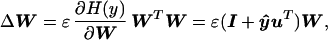
The ICA algorithm we use (5, 9) (Fig. 1) is based on an “infomax” neural network (10, 11). It finds, by stochastic gradient ascent, a matrix, W, which maximizes the entropy (12), H(y), of an ensemble of “sphered” (zero-mean) input vectors {x_s}, linearly transformed and sigmoidally compressed (u = Wx_s, y = g(u)). The “unmixing” matrix W performs component separation, while the sigmoidal nonlinearity g() provides necessary higher-order statistical information. Sphering of the input data (13) (x_s = Sx, where S = 2 〈x x^T〉^−1/2) speeds convergence.

Figure 1.

Schematic overview of ICA of EEG data. (A) (Upper) Averaged (or single) EEG epochs, x, recorded from multiple scalp sites are used to train an “unmixing” weight matrix, W, so as to maximize the entropy of the nonlinearly transformed output, g(Wx). (Lower) After training, rows of the trained weight matrix, W, are linear spatial filters decomposing the input data into the independent activities of the ICA components. Rows of the product of W and the input data, x, are the activation waveforms of the ICA components, while columns of the inverse weight matrix, W⁻¹, map their projections onto the scalp electrodes. (B) (Inset) Schematic illustration of ICA decompositions of a simulated evoked response, recorded at two electrodes (A and B), summing the activity of two temporally independent response sources (#1 and #2) with arbitrary (focal or diffuse) spatial distributions. (Upper) Scatterplot of potentials recorded at the two electrodes, showing the response as a two-dimensional trajectory. In this plot, the activity of source #1 alone would lie on the near-vertical axis ICA-1; the activity of source #2 alone would lie on the near-horizontal (but not orthogonal) axis ICA-2. If the time courses of activation of the two brain networks are independent of one another, the summed output of sources #1 and #2 will, over time, fill the dashed parallelogram. The first principal component of the data (PCA-1) indicates the direction of maximum data variance, but neither this nor the second principal component orthogonal to it identifies either of the independent components. (Lower) The ICA algorithm finds the directions of the two axes (ICA-1, ICA-2) by maximizing the entropy of the data linearly transformed to the ICA component axes and nonlinearly transformed using a logistic sigmoid. The linear transformation and sigmoidal nonlinearity rotates and spreads the data to fill the dashed square as evenly as possible, whereas in the original (A, B) space (above), the data remain within an oblique parallelogram.

W is then initialized to the identity matrix (I) and iteratively adjusted using small batches of data vectors (normally 10 or more) drawn randomly from {x_s} without substitution, according to

1

where ɛ is the learning rate (normally less than 0.01) and vector ŷ has elements ŷ_i = (∂/∂u_i)ln(∂y_i/∂u_i). The (W^TW) “natural gradient” term in the update equation (14, 15) avoids matrix inversions and speeds convergence by normalizing the variance in all directions.

We use the logistic nonlinearity, g(u_i) = (1 + exp(−u_i))⁻¹, which gives a simple update rule, ŷ_i = 1 − 2y_i, and biases the algorithm toward finding sparsely activated or super-Gaussian independent components with positive kurtosis (17), consonant with the assumption that ERPs are composed of one or more overlapping series of brief activations within spatially fixed brain networks performing separable stages of stimulus information processing. The algorithm is able to accurately decompose sums of components with skewed distributions even without making use of nonlinearities specifically tailored to them (5).

The ICA algorithm is easily implemented and computationally efficient. The present implementation does not require matrix inversions, making it practical for use on data from a hundred or more channels. The number of time points needed for the method may be as few as several times the number of recording channels, which in turn must be at least equal to the number of components to be separated. The rows of the output data matrix, u, are the activation waveforms of the ICA components, while the columns of the inverse matrix, (WS)⁻¹, of the overall transformation, WS, give the projection strengths of the respective components onto the scalp sensors. The data accounted for by the ith component are the outer product, (WS)_i⁻¹u_i, of the ith component activation with the ith column of the inverse matrix. Scaling information is distributed between the activation waveforms, u_i, and the maps, (WS)⁻¹, hence relative component strengths can be compared only by means of their projections (WS)_i⁻¹u_i. Note that care must be taken in interpreting decompositions of data sets in which the channel means are far from the baseline means. The ICA algorithm we use is one of a family of algorithms that exploit independence to perform blind separation (9, 14, 15, 17–21).

Application to Evoked Response Decomposition.

The ICA algorithm was applied to two 14-channel, 1-s (312-point) averaged ERPs time locked to detected and undetected targets, respectively, presented in an experiment in which the subject responded by pressing a button each time he heard a weak, slow-onset noise-burst [mean rate, 10/min; duration, 350 ms; rise time, 150 ms; intensity, 6 decibel (dB) sensation level] embedded in a continuous (62-dB) noise background containing a 39-Hz click train producing a steady-state response (SSR) (22). Target noise-bursts were presented in half the intervals between brief nontarget tones (50 ms, 72 dB, 568 Hz, stimulus-onset asynchrony 2–4 s). Further details have been reported elsewhere (23).

EEG data were collected from 13 scalp electrodes referred to the right mastoid, and from a bipolar diagonal electrooculographic placement with a sampling rate of 312.5 Hz and an analog pass band of 0.1–100 Hz. During the 28-min session, the subject experienced variably increasing drowsiness while his target detection rate declined from 100% to 40%. After rejecting trials containing electrooculographic (EOG) potentials larger than 70 μV, brain responses to detected and undetected targets were averaged separately, giving two 312-point ERPs.

ICA decomposition was performed simultaneously on all 624 time points of both ERPs by using Matlab 4.21 on a Sun HyperSparc 125-MHz processor. The learning batch size was 10. Initial learning rate, ɛ, was 0.006. Learning rate was gradually reduced to 10⁻⁶ during 50 training iterations taking 7 s of computer time. The input data are available via http with a package of Matlab routines for performing the analysis.‖

RESULTS

The two responses to detected and undetected targets (Fig. 2A) contained the standard auditory response peaks N1, P2, and N2, although the N1 peak was indistinct, most probably because of the long rise time of the noise-burst stimulus and the variable noise background. As expected from sleep studies of auditory evoked responses (24), the P2 and N2 peaks were larger and had longer latencies in response to undetected targets. The detected-target response also had a parietal P3 component (quite small in this subject), and both responses contained a robust 39-Hz SSR in all channels. The EOG channel showed some residual ocular activity spreading into frontal sites (see, e.g., Fpz). Absolute correlations between channels averaged 0.604 (range: 0.001 to 0.987).

Figure 2.

Decomposition of an ERP data set. (A) Averaged evoked responses at 14 scalp channels from one subject in a sustained auditory detection experiment (23) to detected (blue traces, 209 epochs) and undetected (red traces, 81 epochs) slow-onset noise-burst targets. (B) Activation wave forms of the resulting 14 ICA components during the detected (blue traces) and undetected (red traces) response epochs. Seven components (ICA-1 to ICA-7) are predominantly activated for a period of 50–300 ms during one or the other response. Three more ICA components (ICA-8 to ICA-10) compose the auditory SSR (22) to a click train presented throughout the experiment at one-eighth the EEG sampling rate. The remaining four ICA components (ICA-11 to ICA-14) presumably sum activity of multiple weak brain and extra-brain sources.

The ICA algorithm was used to simultaneously decompose the two 1-s ERPs into 14 ICA components whose activation waveforms are shown in Fig. 2b. Although the algorithm used no temporal sequence information, seven of the ICA components (ICA-1 to ICA-7) were active in a single 50- to 300-ms interval in one of the response conditions. One of these (ICA-4) was active in both conditions. Three more ICA components (ICA-8 to ICA-10) were predominantly periodic at the 39-Hz SSR driving rate. Absolute residual correlations between activation waveforms of these 10 ICA components averaged 0.034, ranging from 0.0001 to 0.143. Projection of these 10 components onto the scalp array accounted for 96.8% of total response variance. Four remaining ICA components (ICA-11 to ICA-14) had higher residual correlations (mean 0.093, range 0.009 to 0.207) and more complex scalp maps (not shown), suggesting they accounted mainly for residual EEG and ocular and muscle activity.

Fig. 3 A and B shows projections of the first seven components to selected scalp electrodes. The detected-target P2 and P3 peaks and the undetected-target P2 were accounted for by single ICA components, while the algorithm decomposed the N2 peak in each response into two or more ICA components. Maps of the individual component scalp projections contained one or two spatial extrema and clearly distinguished components having central, frontal, and periocular foci, even when these appeared to form a single broad peak in the response waveforms at some sites (e.g., ICA-5 to ICA-7). Component ICA-2 accounted for both the detected-target P3 waveform at site Pz and the parallel late negativity at site Fpz. A component with similar time course and topography was found for other subjects in the experiment (Fig. 3D). Component ICA-4 accounted for much of the P2 and early-N2 complex in the detected-target response, but only the central-P2 peak in the undetected-target response.

Figure 3.

Scalp distributions of the ICA components. (A) Projected activity of components ICA-1 to ICA-4 (colored traces) superimposed on the scalp wave forms of the detected-target response (black traces) together with interpolated topographic maps of the component projections (25). Component ICA-2 (green traces) accounts for the central parietal positivity near 450 ms (labeled P3) as well as the concurrent prefrontal positivity at Fpz, whereas the central negativity near 400 ms (labeled N2) includes the activity of component ICA-4 (red traces) which has a different scalp distribution (map scaling ± 6 μV). (B) Projected scalp activity of components ICA-4 to ICA-7 (colored traces) superimposed on the scalp wave forms of the undetected-target response (black traces). The positive central peak near 300 ms (labeled P2) is accounted for by a single component ICA-4 (red traces), whereas the succeeding frontal negativity (labeled N2) is decomposed by the algorithm into three other components (ICA-5 to ICA-7) having central, frontal, and periocular topographies, respectively (map scaling ± 12 μV). (C) The ICA algorithm decomposes the 39-Hz auditory SSR in the detected-target response into three components (ICA-8 to ICA-10) derived from the detected-target ERP (Fig. 2A) by averaging 39 successive 25.6-ms (8-point) ERP time segments. The leftmost traces show the whole SSR at all 14 channels, the right traces, the projected time wave forms and scalp projections (scaled individually) of the three ICA components. The largest component, ICA-8, has a bilateral frontotemporal scalp distribution, as expected (26), while component ICA-9 has a bilateral parietal scalp distribution and component ICA-10 projects mainly to EOG and prefrontal channels. (D) Time courses and scalp topographies of corresponding ICA-2 components obtained in separate decompositions of detected-target responses in two separate sessions from two subjects (right columns) and from the grand-mean detected-target response for 11 subjects (left column). Note the nearly identical time courses (right traces) and scalp maps.

Fig. 3C shows averaged single-cycle SSRs computed by averaging all SSR cycles in the detected-target ERP and in the scalp projections of the three periodic ICA components. SSR waveforms for all 14 channels are superimposed. Above each of the three ICA SSR components is the map associated with each component. The map of the largest component (ICA-8) strongly resembled the topography of the whole SSR at its amplitude peak (not shown). Components ICA-9 and ICA-10 accounted for differences in SSR topography at other time points.

Stability of the Decomposition.

Nearly identical ICA components were recovered from evoked responses collected on different days from the same subject, and similar ICA components from different subjects in the same experiment (Fig. 3D). The activation waveforms and scalp maps of the ICA components with largest projected activities were relatively robust to changes in initial weights, the number of training conditions, and even the number and placement of electrodes. For example, decomposing the data in Fig. 2A by using arbitrary subsets of 11 of the 14 channels gave components whose activations and scalp projections correlated 0.9 or above with ICA components 1, 4, 5, 6, 8, and 9 of Fig. 2B.

ICA decompositions of electric and magnetic evoked responses to a variety of stimuli from several experiments (unpublished) proved similar in character and stability. The algorithm is particularly effective at detecting common response topography in multiple response conditions and at quantifying differences between conditions in activation strength of multiple components.

Relation to Traditional Peak Analysis.

ERP components usually are identified with individual event-related response peaks (e.g., N1, P2, N2, etc.) which were first supposed to represent the activities of brain areas involved in discrete stages of information processing. However, even the peaks of a response waveform may sum the spatially and temporally overlapping activities from two or more brain areas with different time courses of activation (27). When this happens, the scalp topography of the response appears to move continuously even when the brain locations of the active generators are fixed, producing different peak latencies at each scalp site. This is incompatible with the assumption that each peak represents a single response component arising in a fixed brain area. ICA accounts for channels differences in ERP peak latencies by decomposing the activity under each peak into two or more ICA components, each having a spatially fixed scalp topography.

Relation to PCA.

Another linear transformation method previously proposed for ERP decomposition (4), PCA, finds orthogonal directions of greatest variance in the data, whereas ICA finds nearly temporally independent (not just uncorrelated) components whose maps may be nonorthogonal (Fig. 1B). Principal components of data generated by temporally sparse and independent, but spatially nonorthogonal, sources will be linear combinations of activity in all the sources, whereas ICA components of the data will individually identify the larger sources (28). The proposed Varimax extension of the PCA method rotates the PCA vectors to maximize the variance of their activation waveforms (4). However, the relevance of this criterion to ERP genesis is unclear. Applying PCA to the ERP data in Fig. 2A, either alone or followed by Varimax rotation, produced components active throughout both responses (unpublished) with minimal correspondence to the ICA components. When evoked brain activity arises through temporally distinct or partially overlapping activations of independently active neural populations, then ICA appears to be a more appropriate method for separating their contributions to scalp data.

DISCUSSION

The exploratory use of ICA decomposition for ERP analysis is based on three assumptions: (i) that summation at scalp electrodes of potentials arising in different brain areas is linear; (ii) that ERPs are largely the sum of relatively brief activations in a restricted set of spatially stable brain areas, networks, or neural populations; and (iii) that the time courses of activation are largely temporally independent. The first two assumptions appear reasonable. The third assumption limits the decomposition to temporally independent components.

To explore the strengths and limitations of the method, we ran a number of numerical simulations in which 600-point signals recorded from the cortex of a patient during preparation for operation for epilepsy were projected to simulated scalp electrodes through a three-shell spherical model (28, 29). We used electrocorticographic data in these simulations as a plausible best approximation to the temporal dynamics of the unknown ERP brain generators. Results confirmed that the ICA algorithm could accurately identify the activation waveforms and scalp topographies of relatively large and more temporally independent simulated sources, even in the presence of a large number of small and temporally independent simulated sources.

However, given simulated ERP activity arising from separate brain generators whose time courses of activation were substantially correlated, the algorithm parsed the resulting continuously varying scalp responses into distributed activity within overlapping subsets of the simulated sources (28). Similarly, SSR components ICA-8 and ICA-9 (Fig. 3C) collected synchronous bilateral SSR activity instead of splitting it into components with left- and right-sided topographies, and the neural populations generating the activities accounted for by two spatially overlapping components, for example ICA-4 and ICA-5 (Fig. 3B), might not be disjoint, since their scalp distributions are so similar. More generally, given data summing components (however defined) that are not temporally independent, spatially fixed, or sparsely activated, or whose number is not the same as the number of data channels, the algorithm will not reproduce the original component distribution, and other linear blind separation algorithms may produce somewhat different results.

The range of ERP components that can be separated by the algorithm is illustrated by the single broad component (ICA-2), accounting for the posterior P3 response to detected targets as well as the accompanying anterior negativity (Fig. 3A) and the three near-periodic ICA components (ICA8, ICA-9, ICA-10) that together accounted for 95.3% of the total SSR (Fig. 3C). This ICA decomposition of the auditory SSR into three spatially fixed components contrasted sharply with a previously proposed interpretation that the nonstationary SSR reflects a moving crest of activity sweeping through cortex every 25 ms (30). By itself, however, ICA cannot be used to decide between these or other source models (26, 31).

CONCLUSIONS

ICA decomposition opens a new and potentially useful window into complex event-related brain data that can complement other analysis techniques. Further research will be required to fully assess the value and limitations of temporal independence as a segregation criterion. Blind separation by ICA decomposition appears promising for multidimensional measurement of the effects of experimental variables on electric and magnetic evoked-response components representing rapid and discrete stages of brain information processing, particularly when these overlap in scalp distribution. The method may be especially effective for comparing the activations of brain response components that are differentially activated in several related stimulus and cognitive task conditions. Although it may be difficult to locate ICA components within the brain on the basis of their time courses and scalp projections, ICA decomposition might nonetheless prove useful for preprocessing data prior to applying source localization algorithms. ICA decomposition may be useful as well for observing event-related changes in the spatial structure of correlated ongoing EEG activity in multiple brain areas (32–36). The method should be equally applicable to magnetoencephalographic (MEG) data, and it can be generalized to track changes in the spatial structure of EEG or MEG activity in different brain states (8).

ABBREVIATIONS

EEG

electroencephalographic

ERP

event-related potential

ICA

independent component analysis

PCA

principal component analysis

SSR

steady-state response

References

- 1.Nunez P L. Electric Fields of the Brain. New York: Oxford Univ. Press; 1981. [Google Scholar]
- 2.Scherg M, Von Cramon D. Electroencephalogr Clin Neurophysiol. 1986;65:344–360. doi: 10.1016/0168-5597(86)90014-6. [DOI] [PubMed] [Google Scholar]
- 3.Dale A M, Sereno M I. J Cogn Neurosci. 1993;5:162–176. doi: 10.1162/jocn.1993.5.2.162. [DOI] [PubMed] [Google Scholar]
- 4.Chapman R M, McCrary J W. Brain Lang. 1995;27:288–301. [Google Scholar]
- 5.Bell A J, Sejnowski T J. Neural Comput. 1995;7:1129–1159. doi: 10.1162/neco.1995.7.6.1129. [DOI] [PubMed] [Google Scholar]
- 6.Snyder A Z, Abdullaev Y G, Posner M I, Raichle M E. Proc Natl Acad Sci USA. 1995;92:1689–1693. doi: 10.1073/pnas.92.5.1689. [DOI] [PMC free article] [PubMed] [Google Scholar]
- 7.Hillyard S A, Munte T F. Percept Psychophys. 1984;36:185–198. doi: 10.3758/bf03202679. [DOI] [PubMed] [Google Scholar]
- 8.Makeig S, Bell A J, Jung T-P, Sejnowski T J. Advances in Neural Information Processing Systems. 1996;8:145–151. [Google Scholar]
- 9.Bell A J, Sejnowski T J. Proceedings of the International Symposium on Nonlinear Theory and Applications, Las Vegas. Vol. 1. 1995. pp. 43–47. [Google Scholar]
- 10.Linsker R. Neural Comput. 1992;4:691–702. [Google Scholar]
- 11.Nadal J-P, Parga N. Network. 1994;5:565–581. [Google Scholar]
- 12.Cover T M, Thomas J A. Elements of Information Theory. New York: Wiley; 1991. [Google Scholar]
- 13.Bell A J, Sejnowski T J. Network: Computation in Neural Systems. 1996;7:261–266. [Google Scholar]
- 14.Cichocki A, Unbehauen R, Rummert E. Electron Lett. 1994;30:1386–1387. [Google Scholar]
- 15.Amari S, Cichocki A, Yang H H. Advances in Neural Information Processing Systems. 1996;8:757–763. [Google Scholar]
- 16.Olshausen B. Center for Biological and Computational Learning Paper. Massachusetts Institute of Technology, Cambridge, MA: Dept. Brain and Cognitive Sciences; 1996. , No. 138. [Google Scholar]
- 17.Comon P. Signal Processing. 1994;36:287–314. [Google Scholar]
- 18.Jutten C, Herault J. Signal Processing. 1991;24:1–10. [Google Scholar]
- 19.Karhunen J, Oja E, Wang L, Vigario R, Joutsenalo J. IEEE Trans Neural Networks. 1997;8:486–504. doi: 10.1109/72.572090. [DOI] [PubMed] [Google Scholar]
- 20.Cardoso J-F, Laheld B. IEEE Trans Signal Proc. 1996;44:3017–3030. [Google Scholar]
- 21.Lee T-W, Sejnowski T J. Proceedings of the Fourth Joint Symposium on Neural Computation. Vol. 7. Univ. of California San Diego: Institute for Neural Computation; 1997. pp. 132–139. [Google Scholar]
- 22.Galambos R, Makeig S, Talmachoff P. Proc Natl Acad Sci USA. 1981;78:2643–2647. doi: 10.1073/pnas.78.4.2643. [DOI] [PMC free article] [PubMed] [Google Scholar]
- 23.Makeig S, Inlow M. Electroencephalogr Clin Neurophysiol. 1993;86:23–35. doi: 10.1016/0013-4694(93)90064-3. [DOI] [PubMed] [Google Scholar]
- 24.Van Sweden B, Van Dijk J G, Caekebeke J F. Neuropsychobiology. 1994;29:152–156. doi: 10.1159/000119078. [DOI] [PubMed] [Google Scholar]
- 25.Perrin F, Pernier J, Bertrand O, Echallier J F. Electroencephalogr Clin Neurophysiol. 1989;72:184–187. doi: 10.1016/0013-4694(89)90180-6. [DOI] [PubMed] [Google Scholar]
- 26.Pantev C, Elbert T, Makeig S, Hampson S, Eulitz C, Hoke M. Electroencephalogr Clin Neurophysiol. 1993;88:389–396. doi: 10.1016/0168-5597(93)90015-h. [DOI] [PubMed] [Google Scholar]
- 27.Naatanen R, Picton T. Psychophysiology. 1987;24:375–425. doi: 10.1111/j.1469-8986.1987.tb00311.x. [DOI] [PubMed] [Google Scholar]
- 28.Makeig S, Jung T-P, Ghahremani D, Sejnowski T J. Tech. Rep. INC. Univ. of California San Diego: Institute for Neural Computation; 1996. , No. 9606. [Google Scholar]
- 29.Ghahremani D, Makeig S, Jung T-P, Bell A J, Sejnowski T J. Tech. Rep. INC. San Diego: Institute for Neural Computation; 1996. , No. 9601. [Google Scholar]
- 30.Llinas R, Ribary U. Proc Natl Acad Sci USA. 1993;90:2078–2081. doi: 10.1073/pnas.90.5.2078. [DOI] [PMC free article] [PubMed] [Google Scholar]
- 31.Ribary U, Ioannides A A, Singh K D, Hasson R, Bolton J P, Lado F, Mogilner A, Llinas R. Proc Natl Acad Sci USA. 1991;88:11037–11041. doi: 10.1073/pnas.88.24.11037. [DOI] [PMC free article] [PubMed] [Google Scholar]
- 32.Bullock T H, McClune M S, Achimowicz J Z, Iragui-Madoz V J, Duckrow R B, Spencer S S. Proc Natl Acad Sci USA. 1995;92:11568–11572. doi: 10.1073/pnas.92.25.11568. [DOI] [PMC free article] [PubMed] [Google Scholar]
- 33.Gevins A. Brain Topography. 1996;8:189–199. doi: 10.1007/BF01184769. [DOI] [PubMed] [Google Scholar]
- 34.Wackermann J, Lehmann D, Michel C M, Strik W K. Int J Psychophysiol. 1993;14:269–283. doi: 10.1016/0167-8760(93)90041-m. [DOI] [PubMed] [Google Scholar]
- 35.Rappelsberger P, Pfurtscheller G, Filz O. Brain Topography. 1994;7:121–127. doi: 10.1007/BF01186770. [DOI] [PubMed] [Google Scholar]
- 36.Venkatesh N M, Fetz E. J Neurophysiol. 1996;76:3968–3982. doi: 10.1152/jn.1996.76.6.3968. [DOI] [PubMed] [Google Scholar]