Pulmonary fissure segmentation on CT

Abstract

A pulmonary fissure is a boundary between the lobes in the lungs. Its segmentation is of clinical interest as it facilitates the assessment of lung disease on a lobar level. This paper describes a new approach for segmenting the major fissures in both lungs on thin-section computed tomography (CT). An image transformation called “ridge map” is proposed for enhancing the appearance of fissures on CT. A curve-growing process, modeled by a Bayesian network, is described that is influenced by both the features of the ridge map and prior knowledge of the shape of the fissure. The process is implemented in an adaptive regularization framework that balances these influences and reflects the causal dependencies in the Bayesian network using an entropy measure. The method effectively alleviates the problem of inappropriate weights of regularization terms, an effect that can occur with static regularization methods. The method was applied to segment and visualize the lobes of the lungs on chest CT of 10 patients with pulmonary nodules. Only 78 out of 3286 left or right lung regions with fissures (2.4%) required manual correction. The average distance between the automatically segmented and the manually delineated “ground–truth” fissures was 1.01 mm, which was similar to the average distance of 1.03 mm between two sets of manually segmented fissures. The method has a linear-time worst-case complexity and segments the upper lung from the lower lung on a standard computer in less than 5 min.

1. Introduction

With the widespread use of computed tomography (CT) and multidetector CT scanners, large volumes of data reconstructed in thin sections can be produced. These capabilities are not fully utilized due to the large amount of data that needs to be analyzed. Therefore, automatic or semi-automatic image analysis systems are being developed to assist radiologists not only in detection but also qualitative and quantitative analysis of lung pathology while minimizing repetitive and tedious aspects of image interpretation (Ko and Naidich, 2004). To become reliable and useful clinical tools for chest CT analysis, image-based diagnosis systems must be able to segment and model the lung and its associated structures accurately. A structure with important implications for the segmentation of local areas within the lung is the pulmonary fissure, a three-dimensional (3D) boundary surface between the lobes of the lung. The left lung has two lobes separated by a major fissure, and the right lung has three lobes separated by one minor, or horizontal, and one major, or oblique, fissure. This paper describes a method for segmenting the major fissure on thin-section CT.

Our objective was to develop a fissure segmentation method that is computationally efficient so that radiologists need not perform the time-consuming task of identifying the fissure in an entire CT scan. Such a method may have a key role in computer-aided diagnosis systems for both the diagnosis and assessment of malignant and benign lung disease. In particular, as structures that abut the fissures are frequently pulmonary nodules, identification of the fissure might benefit existing image analysis systems for detection (Brown et al., 2001; Ko and Betke, 2001; Shen et al., 2002; Chang et al., 2004; Farag et al., 2004), segmentation (Mullally et al., 2004; Kuhnigk et al., 2004; Okada et al., 2004), and registration (Betke et al., 2003) of nodules which can be an early manifestation of lung cancer. The fissure could also be used as an additional reference to determine the position of a tumor that moves with respiration during radiation treatment and thus reduce the amount of undesirable radiation to surrounding healthy tissue. This may benefit motion-adaptive radiotherapy (Gierga et al., 2004), 4D-CT treatment planning (Rietzel et al., 2003), and image-guided robotic radiosurgery (Adler et al., 1999). Moreover, since the proposed fissure segmentation system can provide a visualization of a patient’s upper and lower lungs, it could be incorporated in teaching software for medical professionals, such as interactive anatomy atlases that provide 3D visualizations of the human body, e.g. (Golland et al., 1999; Kikinis et al., 1996).

A fissure is formed when the visceral pleura of adjacent lobes contact each other, with thickness on the order of 0.2 mm. On CT images of 1–3 mm thickness, the fissure can often be observed as a thin curve with high attenuation values compared to the surrounding tissues (Fig. 1(a)) (Webb et al., 2001). When a CT scan is viewed in the axial plane from the upper thorax to the lower thorax, the cross-section of the major fissure, spanning from the medial to the lateral side of the lung, appears to move from the posterior to the anterior in both lungs (Fig. 1(e)). This paper follows common practice and uses the term “fissure” to refer to the fissure cross-section on axial CT sections, where applicable.

Fig. 1.

Appearances of the major fissure on thin-section CT: (a) fissures appear as thin curvilinear opacities in both lungs; (b)–(d) three sample regions with fissure cross-sections. Fissure fragments are circled in (c); (e) sagittal view of 3D reconstruction of right lung with the segmentation of the major fissure, which separates the surface of the right lung into the upper and lower parts.

On CT, a fissure can have a variety of appearances, which makes its detection and segmentation challenging. Due to respiratory and cardiac motion, as well as partial volume effect, a fissure often appears as a ribbon-like structure, several pixels wide (Fig. 1(b)), rather than the more typical configuration of a thin curvilinear opacity with sharp edges (Fig. 1(a)). When the fissure appears as a ribbon structure, it forms locally bright “ridges” in the axial images and its exact width is difficult to determine. Moreover, frequently fissures are incomplete on CT (Fig. 1(c)) and lobes also have been described to be partially fused (Glazer et al., 1991). Detection and segmentation of the fissure is further complicated by “clutter”, i.e., structures that are located adjacent to the fissure, such as small vessels or nodules. Lastly, the image may also be affected by noise introduced by the imaging process. Our objective was to develop a fissure segmentation method that is robust, i.e., can handle the range of fissure appearances described above.

A large body of the literature has been published on segmentation techniques (Haralick and Shapiro, 1985; Pham et al., 2000), however, few systems have addressed the problem of segmenting the fissure. Previous methods and our proposed method have primarily been directed towards thin-section CT. An exception is the fissure segmentation method by Wang et al. (2002) which was applied to thicker section diagnostic CT (5–10 mm thick sections). Kubo et al. (2001) described detection of major fissures on 1-mm CT sections on a per-section basis. Each CT image was converted into a binary image with a fixed threshold of −300 Hounsfield Units (HU) and then analyzed with morphological operations. Kuhnigk et al.’s method (Kuhnigk et al., 2003) first segmented the vascular tree from the lung parenchyma on chest CT, and then enhanced the brightness of non-vessel voxels based on their distance to the vasculature. The resulting images were processed by an interactive watershed algorithm that achieved the segmentation of the lobes of the lung. Their method relies on accurate vascular segmentation, which is however very difficult to achieve in general. No local shape constraints from neighboring sections or global lung models were used in the above methods (Kubo et al., 2001; Kuhnigk et al., 2003). Zhang et al. (2006) and Zhang (2002) analyzed 1.2–3-mm CT sections using a “ridge operator” to enhance the fissural contrast; in their method, a pulmonary atlas was used to initialize the fissure segmentation process, then a region of interest containing the fissure was determined in each section from segmentation of the previous axial image. A fuzzy reasoning approach followed by a graph search was then applied to the regions of interest to segment the major fissure section by section. The shape constraints from the atlas were used for the final fissure detection as well. Automatic segmentation of the minor fissure has not been well studied yet in previous work (Wang et al., 2002; Kubo et al., 2001; Kuhnigk et al., 2003; Zhang et al., 2006; Zhang, 2002).

Difficulties with existing threshold-based techniques for fissure segmentation relate to the variation of fissure attenuation values among sections and within sections (Fig. 1(a)–(d)). A single fixed threshold on attenuation cannot be used to identify fissure pixels and distinguish them from surrounding clutter (Fig. 1(c)). Its use would result in disjointed fissure fragments. It becomes particularly difficult to identify the disjointed fragments as belonging to the same fissure. Similar issues would arise if other low-level image processing methods such as the Canny edge detector (Canny, 1986) were applied.

Many higher-level image analysis methods have been developed for segmenting the objects that have a similar two-dimensional (2D) appearance as fissures, for instance, for road detection (Geman and Jedynak, 1996), tongue tracking (Akgul et al., 1999), and, most notably, vessel extraction (Aylward and Bullitt, 2002; Aylward et al., 1996; Frangi et al., 1998; Hinz et al., 2001; Koller et al., 1995; Krissian et al., 2000; Lorigo et al., 2000; Vasilevskiy and Siddiqi, 2001). Several methods for vessel segmentation perform eigenvalue analysis of the Hessian matrix of the image intensities (Aylward and Bullitt, 2002; Aylward et al., 1996; Frangi et al., 1998; Koller et al., 1995; Krissian et al., 2000). Koller et al. (1995), for example, used such a technique to define multiscale filters to detect vessel structures in 2D images. Another example is the work by Aylward and Bullitt (2002), Aylward et al. (1996) who extracted 3D vessel structures by detecting their “core”, i.e., their medial loci (Damon, 1999; Pizer et al., 1998). Their method was based on a gradient descent search that analyzed the eigenvalues of the Hessian matrix on each voxel. Other vessel segmentation methods (Hinz et al., 2001; Lorigo et al., 2000; Vasilevskiy and Siddiqi, 2001) have been based on a widely known technique, the “snake” or active contour method (Kass et al., 1987) that used a deformable closed-curve spline contour to capture the boundary of an object in an iterative energy minimizing process. The deformation of the active contour was guided by user-introduced constraints, for example, a smoothness assumption on the object shape, and by properties of the image data in the region of interest. Subsequent methods (Berger, 1990; Cohen and Kimmel, 1997; Mortensen and Barrett, 1995; Williams and Shah, 1992) extended the active contour method (Kass et al., 1987) to detect open-curve boundaries with various degrees of human interactions. Other extensions were level set methods (Caselles et al., 1997; Kichenassamy et al., 1995; Malladi et al., 1995), which can be used to recognize multiple objects simultaneously, even under large variability of object topology. Several works (e.g., Paragios and Deriche, 2002; Yezzi et al., 1999) evolved the object contour based on the statistics of local image regions instead of image gradients. Geometric-flow methods have been developed to segment blood vessels by evolving the surfaces based on the curvatures of vessel centerlines (Lorigo et al., 2000) or by moving the surface points such that the flux of the image gradient vector field is maximized (Vasilevskiy and Siddiqi, 2001).

Addition of boundary smoothness constraints, incorporated into the energy function, enables the original active contour method (Kass et al., 1987) to bridge small gaps in the appearance of the object boundary, which is useful for segmenting a fissure on CT. However, when large gaps are present in an image of a boundary, which occurs for fissures on CT, the active contour method (Kass et al., 1987) often fails. Prior knowledge of boundary shape, however, can bridge such gaps. Previous methods (Leventon et al., 2000; Chen et al., 2002; Cremers et al., 2002; Wang and Staib, 2000) that incorporated prior knowledge of object shape into the contour deformation process required to model the objects as closed curves or surfaces. Motivated by this work and by a contour-growing technique (Berger, 1990), we developed a curve-growing method for fissure segmentation that models the fissure as an open active contour. The proposed technique differs considerably from the vessel segmentation work described above as the 3D structures of fissures and vessels differ significantly, even if their 2D appearances are similar. The method takes advantage of the 3D structure of the fissure as a boundary between the lobes in the lungs: prior shape knowledge obtained from the segmentation results on neighboring sections guides the evolution of the active curve. The contribution of the prior-shape term of the energy function changes adaptively during the curve growing process based on an image entropy formulation. To the best of our knowledge, this formulation is unique. It somewhat relates to the idea of computing the image energy adaptively (Ma and Tagare, 1999; Paragios and Deriche, 2002; Yezzi et al., 1999). Ma and Tagare (1999) used an image energy term that was adaptively computed based on the local arc length of the curve instead of the traditional global term. Approaches based on image-region statistics (Paragios and Deriche, 2002; Yezzi et al., 1999) used mean and variance but not entropy measurements to compute the image energy adaptively.

The proposed fissure segmentation method was integrated as an individual module in a pulmonary image analysis system (Wang et al., 2004) that can automatically segment lung contours on CT. The resulting system can segment the major pulmonary fissures and provide a visualization of the 3D surfaces of the upper and lower lung (Fig. 2). We tested the proposed curve-growing method on 10 thin-section CT scans of 10 patients.

Fig. 2.

System diagram.

2. Methods

This section starts with an overview of the proposed fissure segmentation system. Subsections follow with details of the methods developed for this system.

The main steps of the system are shown in Fig. 3(a). In the initialization step, the fissure is delineated manually on a CT image, the “initialization section”, which is typically located somewhere in the lower half of the lung. If the fissure appears as a clear curve, existing segmentation methods (e.g., Berger, 1990) may also be used for automatic initialization (Fig. 3(c)). The initial fissure curve, denoted as C₀, provides information for automatic segmentation of the fissure in nearby sections in the second step, in which the shape-based curve-growing method are used. The number of axial sections in a thin-section chest CT scan is large, often up to several hundreds. For efficiency reasons, the method may only be applied to a subset of sections. These “key sections” are selected at fixed intervals in the cranio-caudal direction throughout the scan (Fig. 3(c)). A flowchart of the segmentation process applied to the key sections is given in Fig. 3(b). In each key section, the region containing the fissure is first determined. A series of low-level image processing operations then produces a “ridge map” of this region to enhance the appearance of the fissure in the image. The shape-based curve-growing method can then be applied to this map to compute the fissures. Linear interpolation is used to generate the fissures for non-key sections.

Fig. 3.

System diagram of fissure segmentation: (a) overall system; (b) details of processing step 2; (c) locations of initialization, key, and non-key CT sections in the lung.

2.1. Geometric modeling of a fissure and its surrounding region

This section defines a fissure curve geometrically and describes how prior knowledge about its shape can be computed and used to identify its surrounding region. Our definition of this region of interest, called the “fissure region”, ensures that it contains the fissure to be segmented.

The 2D fissure cross-section on a CT section with cranio-caudal coordinate z is referred to as the fissure curve C_z and represented in the form y = C_z(x), where x is the medial–lateral direction or horizontal image axis and y is the anterior–posterior direction or vertical image axis. The fissure curve C can also be represented as a collection of curve segments C = {S₁,…,S_K,…S_N}, where S_K represents the Kth curve segment (Fig. 4(c)). The points on curve segment S_K are denoted by $\{V_K^0,V_K^1,\dots ,V_K^L\}$, where L + 1 is the number of points in S_K. Fissure curves on non-key sections are generated by interpolation. A fissure curve C_z can be interpolated from two fissure curves C_z1 and C_z2 by

Fig. 4.

Fissure curve and fissure region: (a) and (b) two CT key sections I₁ and I₂ with respective fissure curves C₁ and C₂; (c) piecewise linear spline representation of the fissure curve. (d) and (e) Prior curve $C_t^{\ast }$, extrapolated from C₁ and C₂, is used to define the fissure region of height h in current section I_t.

$$C_z(x)=C_{z_1}(x)+r(C_{z_2}(x)-C_{z_1}(x)),$$ (1)

where r = (z − z₁)/(z₂ − z₁) and z₁ < z < z₂. Similarly, Eq. (1) can be used to extrapolate a fissure curve C_z if z₁ < z₂ < z or z < z₁ < z₂.

In step 1 of the fissure segmentation system (Fig. 3(a)), initial curve C₀ is segmented on the initialization section I₀. In step 2, the fissure region of each key section is located. First, the fissure region of the first key section I₁ at distance d below I₀ is determined as follows. The curve C₀ is translated onto I₁ and then translated in the anterior direction by kd, where k is a constant scale factor. When projected into the sagittal plane, gradients of the upper lung surface are typically oriented at an angle to the cranio-caudal axis of about 45°. By choosing k = tan (45°) = 1, we can thus approximate a translation along the gradient direction of the upper lung surface. The translated curve is denoted by $C_1^{\ast }$. Symbol * indicates that the curve provides prior shape information for segmentation of the fissure in I₁. Prior curve $C_1^{\ast }$ is used to define the fissure region of I₁. The region contains all lung voxels of section I₁ with $C_1^{\ast }(x)-\lfloor h/2\rfloor \le y\le C_1^{\ast }(x)+\lfloor h/2\rfloor$, for some constant h (Fig. 4(d)). The fissure region of a subsequent key section I_t can be identified by combining the information of two previously segmented curves, e.g., the initial curve C₀ and the fissure C₁ segmented on I₁. In general, the prior curve $C_t^{\ast }$ on I_t is extrapolated from the curves C₁ and C₂ on some nearest sections I₁ and I₂ using Eq. (1) (Fig. 4) with z₁ < z₂ < z_t or z_t < z₁ < z₂. The fissure region of section I_t is then computed using $C_t^{\ast }$ as in the previous case. Values for the parameters d, k, and h were chosen by experimentation as described in Section 3. The experiments took into account the general size, position, and shape of human lung lobes, as well as the resolution of the given thin-section CT data sets.

2.2. Identifying fissure candidate pixels on ridge map of fissure region

An image enhancement operation was developed to support the detection of fissures on thin-section CT. It is particularly useful as a pre-processing technique when the fissure appears as a curvilinear structure of a certain width. The approach generates a ridge map I_⊓ in three steps (Fig. 5) and then identifies fissure candidate pixels. First, the fissure region I is smoothed by applying a 3 × 3 Gaussian operator G (Jain et al., 1995) such that I_G = I ⊗ G, where ⊗ denotes convolution. Second, based on the convolution of Sobel masks (∇_x, ∇_y) (Jain et al., 1995) with I_G, a map I_∇ = sign (∇_y ⊗ I_G) (|∇_x ⊗ I_G| + |∇_y ⊗ I_G|), containing the signed magnitude of the gradient is defined, where sign( ) is a function returning 1 on a positive input and −1 on a negative. The sign function was chosen so that the gradient map I_∇ can provide directional information about the image gradient in the anterior–posterior direction (y-direction). Third, the ridge operator ⊓ is applied to I_∇ which yields the ridge map

Fig. 5.

Ridge map generation, case 1: top left: fissure region on CT. Right: convolution masks used to generate gradient and ridge maps. Middle: subregion of fissure (black rectangle on left) and its gradient and ridge maps as 3D surfaces that were smoothed by linear interpolation on true values and rendered for better visualization. Left: anterior–posterior cross-sections of gradient and ridge maps with zero-crossings occurring in a two-pixel window. The ridge map maximum occurs at the center pixel of this window, which is a pixel of the fissure cross-section.

$$I_{\sqcap }=\text{sign}({\sqcap }_y\otimes I_{\nabla })(|{\sqcap }_x\otimes I_{\nabla }|+|{\sqcap }_y\otimes I_{\nabla }|).$$ (2)

Since the gradient map I_∇ was defined so that it can maintain directional information, the sign function in the above definition of the ridge map I_⊓ (Eq. (2)) can distinguish high-attenuation ridges from low-attenuation valleys.

Ridge maps significantly enhance the appearance of fissures as can be seen for two examples in Figs. 5 and 6. Ideally, their local maxima of a ridge map along the anterior–posterior direction (y-direction) correspond to the pixels of the fissure on CT. However, some local maxima may represent pixels on non-fissure structures, e.g., vessels, which can be identified by evaluating the orientation of the ridge vector (⊓_x ⊗ I_∇, ⊓_y ⊗ I_∇) at these pixels. Fissure pixels have ridge vectors that point in the direction perpendicular to the fissure curve (y-direction), i.e., [π/4:3π/4], because the fissure is generally aligned in the medial–lateral direction. Pixels on ridges whose ridge vectors point in a direction outside of this range are considered clutter and can be removed. This is done in step 2 of the fissure segmentation system. The connected components of the remaining pixels are computed, and pixels in small components are removed. The remaining pixels are considered candidate pixels for the fissure curve in the proposed curve-growing segmentation methods.

Fig. 6.

Ridge map generation, case 2: here, the gradient changes are smoother than in the example in Fig. 5, so that the anterior–posterior cross-sections of gradient and ridge maps have zero-crossings in a six-pixel window. The ridge map operator also succeeds in this case: the ridge map maxima occur at the center pixels of this window and is a pixel in the fissure cross-section.

The proposed ridge map operator provides a simple and efficient way to enhance the appearance of fissures on CT. Other derivative-based transformations might produce similar enhancements, for example, the work by Koller et al. (1995), Aylward and Bullitt (2002, 1996), Krissian et al. (2000), and Frangi et al. (1998).

2.3. Shape-based curve growing method

In this section, a method for segmenting fissures is described that grows the curve segment by segment, as inWilliams and Shah’s greedy search (Williams and Shah, 1992), in each step locating a curve segment that minimizes an energy function. Our method evaluates the following energy function to estimate the position of the Kth segment of the curve:

$$E_K={\alpha }_K{f}_{\text{shape}}+\beta f_{\text{img}}+\gamma f_{\text{curv}},$$ (3)

where function f_shape measures the shape similarity between current and prior curves, function f_img the “image energy” of the current curve, and function f_curv the curvature of the current curve (detailed definitions are given in Section 2.3.2). Our formulation differs from previous approaches in the literature, e.g. (Berger, 1990; Chen et al., 2002; Leventon et al., 2000; Wang and Staib, 2000; Williams and Shah, 1992), in that we chose an adaptive parameter α_K, in addition to two fixed regularization parameters β and γ, to weigh the contributions of the three terms in the energy function.

The CURVE GROWING ALGORITHM takes as inputs the prior shape curve C* and the image data in the ridge map I_⊓ (Sections 2.1 and 2.2). The original image data I or other transformations of it can also be used, so the subscript ⊓ is dropped in the description of the algorithm. The algorithm locates C by adding curve segments S_K, K = 2,…,N, one at a time, to the initial segment S₁. The method for finding an initial curve segment in step 2 of the algorithm is described in Section 2.3.1. Segment S_K is estimated in step 3–9 by evaluating previously estimated segment Ŝ_K−1, prior curve segments $S_K^{\ast }$ and $S_{K-1}^{\ast }$, and a set of n candidate segments ${\{S_K^i\}}_{i=1}^n$ that collectively define the image region of interest I_K (Fig. 7 and Section 2.3.2). The entropy-based computation of the regularization parameter α_K is described in Section 2.3.3. The computational complexity of the algorithm is linear in the number of pixels of the fissure region.

Fig. 7.

Growing a curve segment: the previously estimated curve segment Ŝ_K−1 is extended from its last point ${\widehat{V}}_{K-1}^L=V_K^0$ with a new segment S̄_K in a direction such that the curvature at $V_K^0$ is the same as the curvature at point $V_K^{\ast 0}$ on the corresponding segments $S_K^{\ast }$ and $S_{K-1}^{\ast }$ of prior curve C*. Segment S̄_K is a candidate segment for S_K. The other candidate segments (dashed lines) surround S̄_K and define a fan-shaped region I_K (light shading). The image values of curve spline points ${\text{V}}_K^0$ and ${\text{V}}_K^{L,i}$ (dark circles) and all non-spline points (white circles, dashed lines) are evaluated of each candidate segment $S_K^i$, i = 1,…,n. A candidate segment is selected as the new curve segment Ŝ_K based on these image values, the curvature value at point $V_K^{\ast 0}$, and the curvature values at point $V_K^0$ computed for the candidate segments.

2.3.1. Curve initialization

The objective of the curve initialization process is to identify an initial curve segment Ŝ₁ among the set $\{S_1^j\}$ of connected components of fissure candidate pixels that were determined by the method described in Section 2.2. This is difficult because, at this early step in the CURVE GROWING ALGORITHM, it is not known whether a particular segment $S_1^j$ belongs to the final fissure curve. The proposed method uses confidence weights to determine if a

CURVE GROWING ALGORITHM (C*,I)

1. Initialize K = 1, length L = 5, sample size n = 7, and regularization parameters β = 0.5 and γ = 0.1.

2. Estimate initial curve segment Ŝ₁.

3. Grow curve C from Ŝ₁ rightwards until right lung boundary is reached by repeating:

4. K = K + 1;

5. Locate curve segment S̄_K to the right of Ŝ_K−1 such that $f_{\text{curv}}({\overline{S}}_K,{\widehat{S}}_{K-1})=f_{\text{curv}}(S_K^{\ast },S_{K-1}^{\ast })$.

6. Define candidate segments ${\{S_K^i\}}_{i=1}^n$ such that S̄_K is middle segment.

7. Compute entropy H(S_K|I_K, Ŝ_K−1) based on samples ${\{S_K^i\}}_{i=1}^n$.

8. Compute regularization parameter α(I_K, Ŝ_K−1) based on H(S_K|I_K, Ŝ_K−1)

9. Estimate curve segment ${\widehat{S}}_K=arg{min}_{S_K^i}[\alpha (I_K,{\widehat{S}}_{K-1})(S_K^i,{\widehat{S}}_{K-1},C_K^{\ast })+\beta f_{\text{img}}(S_K^i)+\gamma f_{\text{curv}}(S_K^i,{\widehat{S}}_{K-1})]$.

10. Grow curve from Ŝ₁ leftwards until left lung boundary is reached (as in step 3–9).

11. Output C.

segment is a fissure or non-fissure segment (Fig. 8(a)). For each segment $S_1^j$, the prior curve C* is translated in the anterior–posterior direction so that it overlays the centroid of $S_1^j$. The resulting curve is denoted by $C_{(j)}^{\ast }$. A confidence weight $W_j={\sum }_{\nu \in C_{(j)}^{\ast }}I(\nu )$ is then calculated for each segment $S_1^j$ by accumulating a normalized ridge map value of each point on curve $C_{(j)}^{\ast }$. The ridge value is normalized by the maximum ridge map value among all pixels with the same medial–lateral position (i.e., same image column). The normalization balances the amount that pixels at different medial–lateral positions (i.e., different columns) contribute to the confidence weights. The segment with the highest confidence weight W_max is selected and identified as the initial curve segment Ŝ₁.

Fig. 8.

Curve initialization: (a) alignments of prior curve C* with candidate segments $\{S_1^j\}$; (b) fissure region on CT (top), candidate segments $\{S_1^j\}$ (white, middle), where the longest segment is circled, and the selected initial curve segment Ŝ₁ (bottom).

2.3.2. Energy function derived by maximum a posteriori estimation

In this section, the energy function used in step 9 of the CURVE GROWING ALGORITHM (Eq. (3)) is derived based on Bayesian estimation theory. The approach is illustrated with Bayesian networks (Pearl, 1988), which have been applied to many applications that involve reasoning processes. A Bayesian network was developed in which the prior shape curve C* and the image data I are random variables that are “causal predecessors” of the random variable C, the curve to be estimated (Fig. 9(a)). Segmenting the curve C is then equivalent to finding the maximum-a-posteriori (MAP) estimate Ĉ that maximizes the conditional probability density p(C|C*,I) for the prior shape C* and the observed image data I (font “roman” is used to denote random variables, font “italics” to indicate that the random variable has taken on a particular value, and symbol ^ to describe that such a value was estimated by the proposed method). Each segment S_K of the curve C is also modeled as a random variable which is assumed to be only dependent on the most recently added curve segment S_K−1 and not on earlier segments. This “Markov assumption” (Pearl, 1988) on consecutive curve segments yields the Bayesian network shown in Fig. 9(b). Segmenting the fissure is then equivalent to finding the curve Ĉ that maximizes of the conditional probability

Fig. 9.

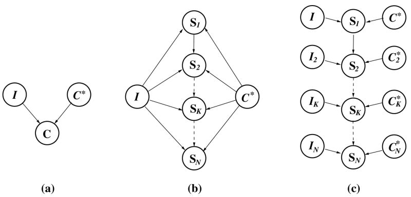
A hierarchy of Bayesian networks for curve growing: (a) random variable C, representing the curve to be estimated, is influenced by prior information about fissure shape C* and image data I; (b) random variable S_K, representing the Kth curve segment to be estimated, is influenced by image data I, prior curve C* and previous curve segment S_K−1; (c) random variable S_K, K = 2,…,N, is influenced by local image data I_K, previous curve segment S_K−1 and the set $C_K^{\ast }$ of corresponding points on the prior curve.

$$\begin{array}{l}p(\text{C}|C^{\ast },I)=p({\text{S}}_1,{\text{S}}_2,\dots ,{\text{S}}_N|C^{\ast },I)\\ =p({\text{S}}_1|C^{\ast },I)p({\text{S}}_2|{\text{S}}_1,C^{\ast },I)p({\text{S}}_3|{\text{S}}_2,C^{\ast },I)\dots \\ \times p({\text{S}}_N|{\text{S}}_{N-1},C^{\ast },I).\end{array}$$ (4)

We assume that the initial curve segment Ŝ₁, estimated as described in Section 2.3.1, maximizes p(S₁|C*,I). It then remains to be explained why each segment Ŝ_K, computed in step 9 of the algorithm, maximizes the conditional probabilities p(S_K|Ŝ_K−1, C*, I), for K = 2,…,N. Each term p(S_K|Ŝ_K−1, C*, I) can be rewritten as $p({\text{S}}_K|{\widehat{S}}_{K-1},C_K^{\ast },I_K)$ to indicate the dependence of S_K on the local attenuation measurements I_K and the set of points $C_K^{\ast }$ on prior curve C* that correspond to the points on segments S_K and Ŝ_K−1 of curve C (Fig. 9(c)). Bayes’ rule yields

$$\begin{array}{l}p({\text{S}}_K|{\widehat{S}}_{K-1},C_K^{\ast },I_K)=p(I_K|{\text{S}}_K,{\widehat{S}}_{K-1})p(C_K^{\ast }|{\text{S}}_K,{\widehat{S}}_{K-1},I_K)\\ \times p({\widehat{S}}_{K-1}|{\text{S}}_K)p({\text{S}}_K)p({\widehat{S}}_{K-1},C_K^{\ast },I_K),\end{array}$$ (5)

where the normalizing factor $p({\widehat{S}}_{K-1},C_K^{\ast },I_K)$ is irrelevant to estimating segment S_K, and where the prior p(S_K) is considered to be uniform. Finding the segment Ŝ_K that maximizes $p({\text{S}}_K|{\widehat{S}}_{K-1},C_K^{\ast },I_K)$ then means finding Ŝ_K that maximizes the product $p(I_K|{\text{S}}_K,{\widehat{S}}_{K-1})p(C_K^{\ast }|{\text{S}}_K,{\widehat{S}}_{K-1},I_K)p({\widehat{S}}_{K-1}|{\text{S}}_K)$. The remainder of this section describes the respective relationships between these three probability functions to the image energy, shape similarity, and curvature terms f_img, f_shape, and f_curv of the energy function.

First, it is reasonable to assume that the curve segment of the fissure should be on the high-attention ridges in the ridge map. The pixels ${\text{V}}_K^0,{\text{V}}_K^1,\dots ,{\text{V}}_K^L$ belonging to the curve segment S_K are therefore likely to have larger ridge values $I({\text{V}}_K^0),\dots ,I({\text{V}}_K^L)$ than neighboring pixels. The sum of attenuation values along the segment can be bounded from above and below by the constants I_max and I_min (±2 × 10⁶ HU). The expression $f_{\text{img}}({\text{S}}_K)=I_{max}-{\sum }_{j=1}^{L}I({\text{V}}_K^j)$ can then be used to define the image energy of segment S_K and to model p(I_K|S_K, Ŝ_K−1) by the truncated exponential density function

$$\begin{array}{l}p(I_K|{\text{S}}_K,{\widehat{\text{S}}}_{K-1})=\rho exp\left(\sum _{j=0}^{L}I({\text{V}}_K^i)-I_{max}\right)\\ =\rho exp(-f_{\text{img}}({\text{S}}_K)),\end{array}$$ (6)

where ρ = 1/(1 − exp(I_min − I_max)) is a constant normalization factor.

Second, the fissure surface changes smoothly in the medial–lateral direction, and thus the curvature is small at each spline point of the fissure curve and zero at each non-spline point (see Fig. 7). The curvature of spline point ${\widehat{V}}_{K-1}^L={\text{V}}_K^0$ can be approximated (Williams and Shah, 1992) by the squared length of the vector ${\widehat{V}}_{K-1}^0+{\text{V}}_K^L-2V_K^0$, which is the difference between vector ${\widehat{V}}_{K-1}^0-{\widehat{V}}_{K-1}^L$ along segment Ŝ_K−1 and vector $V_K^0-{\text{V}}_K^L$ along S_K. Using the curvature expression $f_{\text{curv}}({\text{S}}_K,{\widehat{S}}_{K-1})=\parallel {\widehat{V}}_{K-1}^0+{\text{V}}_K^L-2V_K^0{\parallel }^2$, the conditional probability p(Ŝ_K−1|S_K) is then modeled by the zero-mean Gaussian density function of the square root of the approximated curvature f_curv at point $V_K^0$,

$$p({\widehat{S}}_{K-1}|{\text{S}}_K)=\frac{1}{\sqrt{2\pi }{\sigma }_c}exp\left(-\frac{f_{\text{curv}}({\text{S}}_K,{\widehat{S}}_{K-1})}{s{\sigma }_c^2}\right),$$ (7)

with constant variance ${\sigma }_c^2$.

Third, the fissure surface also changes smoothly in the cranio-caudal direction. The difference between curvature f_curv(S_K,S_K−1) at $V_K^0$ and curvature $f_{\text{curv}}(S_K^{\ast },S_{K-1}^{\ast })$ at corresponding point $V_K^{\ast 0}$ on prior curve segments $S_K^{\ast }$ and $S_{K-1}^{\ast }$ is used to define the shape similarity $f_{\text{shape}}(S_K,S_{K-1},C_K^{\ast })$ of the current and prior curves. The corresponding point $V_K^{\ast 0}$ is found by searching for the closest point on C*, i.e., the point with the smallest Euclidean distance to $V_K^0$ (Fig. 7). Using the shape similarity expression $f_{\text{shape}}(S_K,S_{K-1},C_K^{\ast })={(f_{\text{curv}}(S_K^{\ast },S_{K-1}^{\ast })-f_{\text{curv}}(S_K,S_{K-1}))}^2$, the conditional probability $p(C_K^{\ast }|{\text{S}}_K,{\widehat{S}}_{K-1},I_K)$ is then modeled by the zero-mean Gaussian density function of the square root of the approximated shape similarity f_shape between points $V_K^0$ and $V_K^{0\ast }$,

$$\begin{array}{l}p(C_K^{\ast }|{\text{S}}_K,{\widehat{S}}_{K-1},I_K)=\frac{1}{\sqrt{2\pi }\sigma (I_K,{\widehat{S}}_{K-1})}\\ \times exp\left(-\frac{f_{\text{shape}}({\text{S}}_K,{\widehat{S}}_{K-1},C_K^{\ast })}{2{\sigma }^2(I_K,{\widehat{S}}_{K-1})}\right),\end{array}$$ (8)

where the variance σ₂(I_K, Ŝ_K−1) is modeled as a function of the observed attenuations I_K and the estimated curve segment Ŝ_K−1. Note that modeling this functional dependence allows us to be consistent with the Bayesian network in Fig. 9(c). In particular, the shape similarity measure can only have a small variance in situations, where the attenuation values in region I_K are very similar or, where the curve is not smooth. Conversely, the shape similarity measure can have a large variance in situations, where the fissure curve is smooth or, where there is strong evidence for the location of curve segment S_K in image region I_K. To capture these insights about estimation uncertainty, we propose an entropy formulation for modeling the variance σ²(I_K, Ŝ_K−1) in Section 2.3.3.

The segment Ŝ_K that maximizes $p({\text{S}}_K|{\widehat{S}}_{K-1},C_K^{\ast },I_K)$ (Eq. 5) also maximizes the logarithm of the product $p(C_K^{\ast }|{\text{S}}_K,{\widehat{S}}_{K-1},I_K)p(I_K|{\text{S}}_K,{\widehat{S}}_{K-1})p({\widehat{S}}_{K-1}|{\text{S}}_K)$. This is equivalent to minimizing the sum

$$\begin{array}{l}\frac{1}{2{\sigma }^2(I_K,{\widehat{S}}_{K-1})}{f}_{\text{shape}}({\text{S}}_K,{\widehat{S}}_{K-1},C_K^{\ast })+f_{\text{img}}({\text{S}}_K)\\ +\frac{1}{2{\sigma }_c^2}{f}_{\text{curv}}({\text{S}}_K,{\widehat{S}}_{K-1})\end{array}$$ (9)

of the arguments of the exponential functions in Eqs. (6)–(8). Since the relative weights of the three terms matter rather than their absolute values, the energy function can be rewritten as:

$$\begin{array}{l}\alpha (I_K,{\widehat{S}}_{K-1})f_{\text{shape}}({\text{S}}_K,{\widehat{S}}_{K-1},C_K^{\ast })+\beta f_{\text{img}}({\text{S}}_K)\\ +\gamma f_{\text{curv}}({\text{S}}_K,{\widehat{S}}_{K-1})\end{array}$$ (10)

with regularization parameters α(I_K, Ŝ_K−1), β and γ. The values for the fixed parameters β and γ were chosen by experimentation as described in Section 3, while α(I_K, Ŝ_K−1) is determined as described in the following section.

2.3.3. Adaptive regularization via entropy computation

Ill-suited values for regularization parameters α(I_K, Ŝ_K−1), β and γ can lead to undesirable results of the energy minimization process. For instance, if parameter α(I_K, Ŝ_K−1) is assigned a value that is too large for a situation in which the current and prior fissure shapes are quite different, the shape of prior curve C* may overly influence the estimation of curve Ĉ. On the other hand, if parameter α(I_K, Ŝ_K−1) is assigned a value that is too small, noise or clutter in the image may overly influence the estimation of curve Ĉ. Optimal regularization factors can be learned by various approaches, e.g., a cross-validation method (Li, 1995) that requires a large amount of computation before the segmentation process, and the resulting parameters are then static during the segmentation process. Instead of using such a static regularization mechanism, we propose to determine the values of α(I_K, Ŝ_K−1) adaptively during the curve growing process while parameters β and γ remain fixed.

To derive an expression for adaptive regularization parameter α(I_K, Ŝ_K−1), which is inversely proportional to the variance σ₂(I_K, Ŝ_K−1) of the shape similarity measure, we define the entropy (Shannon, 1948) of S_K, given I_K and Ŝ_K−1:

$$H({\text{S}}_K|I_K,{\widehat{S}}_{K-1})=-\sum _{i=1}^n(p(S_K^i|I_K,{\widehat{S}}_{K-1}){log}_{2}p(S_K^i|I_K,{\widehat{S}}_{K-1})),$$ (11)

where $S_K^i$ is the ith sample of S_K in I_K (Fig. 7) and, where

$$p(S_K^i|I_K,{\widehat{S}}_{K-1})=p(I_K|S_K^i,{\widehat{S}}_{K-1})p({\widehat{S}}_{K-1}|S_K^i)p(S_K^i)/p(I_K,{\widehat{S}}_{K-1}).$$ (12)

The product $p(I_K|S_K^i,{\widehat{S}}_{K-1})p({\widehat{S}}_{K-1}|S_K^i)p(S_K^i)$ can be computed using Eqs. (6) and (7) and $p(S_K^i)=1/n$. The joint probability p(I_K, Ŝ_K−1) is a normalizing constant and equal to $\sum (p(I_K|S_K^i,{\widehat{S}}_{K-1})p({\widehat{S}}_{K-1}|S_K^i))/n$, because, for given I_K and Ŝ_K−1, the summation of $p(S_K^i|I_K,{\widehat{S}}_{K-1})$ must be equal to 1.

Note that the maximum entropy, or the greatest uncertainty in estimating S_K, occurs when $p(S_K^i|I_K,{\widehat{S}}_{K-1})=1/n$ for each of the n samples. The entropy ranges from 0 to logn, and thus H′ = H/logn ranges from 0 to 1. By experiments, we determined that values of this normalized entropy H′ below λ = 0.5 occur when the fissure curve appears clearly in the image region I_K. For such cases, we assigned the value of ε = 0.2 to the adaptive regularization parameter α(I_K, Ŝ_K−1), which ensures that the shape prior has a low weight in the energy computation. For values of H′ above λ = 0.5, i.e., situations with greater uncertainty in estimating S_K, we used a rescaled value of H′, in particular,

$$\alpha (I_K,{\widehat{S}}_{K-1})=max\{\epsilon ,(H({\text{S}}_K|I_K,{\widehat{S}}_{K-1})/logn-\lambda )/(1-\lambda )\},$$ (13)

which ensures that the prior shape has a large weight in the energy computation. Examples of normalized entropy values H′ and corresponding value of α along the fissure curve are given in Fig. 10.

Fig. 10.

Image features, entropy and adaptive regularization: (a) regions of interest in original CT images; (b) ground–truth fissure curves; (c) corresponding ridge maps; (d) normalized entropy H′ along the curve; (e) corresponding value of α along the curve. Ambiguous image features correspond to high uncertainty for curve localization, which is represented as the large values of H′ and α. The corresponding locations in the ridge map and their relevant values in the graph are circled in (c)–(e).

For computational convenience, our current implementation of entropy H(S_K|I_K, Ŝ_K−1) stressed the image influence modeled by $p(I_K|S_K^i,{\widehat{S}}_{K-1})$ and considered the curve smoothness to be less important, i.e., using a uniform distribution for $p({\widehat{S}}_{K-1}|S_K^i)$. As a result, the entropy H(S_K|I_K, Ŝ_K−1) is approximated by computing $-{\sum }_{i=1}^n(p(I_K|S_K^i,{\widehat{S}}_{K-1}){log}_{2}p(I_K|S_K^i,{\widehat{S}}_{K-1}))$ instead of Eq. (11).

3. Experimental results

This section summarizes the results of two kinds of empirical studies: (1) experiments that used the curve-growing method to segment the pulmonary fissures on CT scans of 10 patients, and (2) tests that supported the development of the proposed method, in particular, the selection of parameter values.

The major pulmonary fissures were segmented on 10 1.25-mm-section CT scans of patients with pulmonary nodules (see Table 1). A total of 2890 sections were processed. The average number of sections per CT scan was 288. On average, the number of sections per CT scan with left lung fissures was 174 and with right lung fissures was 155. The curve-growing method was applied to every section of the first five CT scans (processing mode 1) and every third section for the remaining five CT scans (processing mode 2). Fig. 11 shows the lungs of five patients, each with two lobes separated by the major fissures. The results of the curve-growing method on each key section were either confirmed by visual inspection or manually corrected if the method failed to delineate a complete fissure curve. Manual correction took 5–20 s depending on the length of the curve on a given section. The proposed segmentation method was successful in the sense that only 78 out of 3286 left or right lung regions with fissures (2.4%) required manual correction (see Table 1). The degree of automation for a CT scan, computed by the ratio of the number of sections in which a fissure curve was produced without human correction over the total number of sections with fissures, was thus 97.6%, on average.

Table 1.

Results of fissure segmentation on 10 CT scans: automatic segmentation was performed on N_C of the key sections and N_I = N_T − (N_C + N_M) non-key sections

Patient	Number of sections in CT scan	Lung	Number of fissure sections, NT	Number of sections segmented by			Degree of automation $\frac{N_{\text{T}}-N_{\text{M}}}{N_{\text{T}}}$ (%)	Voxel width (mm)	RMS distance (mm)	Standard deviation of distance (mm)
				Curve growing, NC	Manual marking, NM	Interpolation, NI
1	322	Right	195	192	3	–	98	0.74	1.30	1.06
		Left	246	245	1	–	99
2	269	Right	163	159	4	–	98	0.55	1.31	0.85
		Left	181	177	4	–	98
3	274	Right	155	149	6	–	96	0.59	2.15	1.59
		Left	179	173	6	–	97
4	297	Right	164	159	5	–	97	0.57	1.67	1.15
		Left	186	184	2	–	99
5	259	Right	136	132	4	–	97	0.55	1.33	0.81
		Left	179	178	1	–	99
6	233	Right	125	39	2	84	98	0.62	1.05	0.79
		Left	148	46	4	98	97
7	301	Right	135	42	4	89	97	0.54	0.75	0.68
		Left	121	38	3	80	98
8	304	Right	166	51	5	110	97	0.68	0.92	0.77
		Left	148	45	5	98	97
9	307	Right	160	49	5	106	97	1.00	1.50	1.22
		Left	190	61	3	126	98
10	324	Right	146	44	5	97	96	1.00	1.77	1.19
		Left	163	46	6	111	96

Manual segmentation was performed on N_M sections, which includes the initialization section.

Fig. 11.

The lungs of patients 1, 2, 6, 8, and 9 with lobes segmented by the curve-growing method. Each lung surface contour is separated into two parts at the points, where the fissure curve joined the lung contour. For the left lungs, the upper lung contours and segmented fissure curves form the surface of the upper lobe of the lung (light gray) and the lower lung contours and fissure curves form the surface of the lower lobe of the lung (dark gray). The right lungs are visualized similarly, except that each upper lung is a combination of the patient’s right upper lobe and middle lobe as the minor fissure was not segmented.

To evaluate the accuracy of the curve-growing method, we compared the curves delineated by a human expert, which serve as a gold standard, with automatically segmented curves. A distance measure computes the root-mean- square (RMS) value and standard deviation of the distances between all pairs of corresponding points on the curves with the same coordinate value in the medial–lateral direction. Accuracy results based on the distance measure are reported in Table 1. In each CT scan, 20 major fissures, which were segmented automatically, were randomly selected in left or right lung cross-sections. The average RMS value of 1.38 mm and standard deviation of 1.01 mm of the distances between ground and truth curves and these automatically segmented curves were small compared to the average voxel width of the CT image, which was 0.68 mm. We conclude that the fissures segmented by the curve-growing method on average approximates the gold standard closely.

The performance of the proposed segmentation method is illustrated in Figs. 12–16. Intermediate results during the curve-growing process are shown in Figs. 12 and 13. A comparison of curve-growing results with results obtained by using the method in Berger (1990) are shown in Figs. 13 and 14. An example, where manual correction was required is shown in Fig. 15. Cases with large RMS values are shown in Fig. 16.

Fig. 12.

Curve growing example: (a) fissure region with large nodule; (b) prior shape C*, (c) corresponding ridge map and candidate segments before initialization; (d) initial segment after initialization. This segment is chosen instead of the longer one, circled in (c); (e)–(h) intermediate results at iterations 4, 8, 16 and 18.

Fig. 16.

Examples with large RMS distances between ground–truth and segmented curves: (1a–3a) three fissure regions on CT of patient 3 and 4; (1b–3b) automatically (top) and manually (bottom) segmented fissure curves.

Fig. 13.

Comparison of methods: top: intermediate results at iterations 2, 6, 18, 20 and 24. The curve-growing method successfully bypassed the pulmonary nodule. Bottom: results using the method in Berger (1990), which did not bypass the nodule correctly.

Fig. 14.

Challenging segmentation scenarios: (a) seven fissure regions on the original CT images from four patients which include a significant amount of clutter; (b) segmented curves by proposed method; (c) segmented curves by method in Berger (1990); (d) ground–truth curves. While the segmentations in (1b) and (1c) are similar, the results in (2c–7c) are clearly inferior to the curve-growing results in (2b–7b) since the method in Berger (1990) relied on the image intensities only and did not take advantage of prior information about curve shape. Ground–truth for image (7a) was difficult to establish in the region marked by the arrow in (7d). The fissure segmentation in (7b) is more likely than in (7c) based on the segmentation results from neighboring sections.

Fig. 15.

Example, where human correction was required: (1–3) the fissure regions (top) and curves (bottom) on three previously segmented key sections; (4) the fissure region on the current key section. The distance between each key section shown in (1–4) is 2.5 mm; (5) the fissure curve segmented by the proposed method (top) and the manually marked curve (bottom) on the current key section shown in (4); the differences in shape of the segmented curves in sections (1–4) were mainly due to the bright lung structure highlighted by black arrows, which led to an incorrect segmentation on the current key section that required manual correction. The image region marked on (4) by the white arrow indicates the right location of the fissure curve.

The need for manual correction does not differ significantly between the two modes of processing (i.e., without interpolation as reported for patients 1–5 in Table 1 and with interpolation as for patients 6–10); the respective results for the average degree of automation for the two modes were 97.9% and 97.2% (p-value > 0.2). The need for visual inspection, however, differed significantly: on average, 175 sections were segmented by the curve-growing method in mode 1 and only 46 sections in mode 2. On a work station with a 2 GHz dual processor with 2 GB memory, it took 2:35 min to segment the CT scan of patient 6 in mode 1, which included human markings on one section. It took 1:25 min to segment the same CT scan in mode 2, which included human markings on two sections. This timing difference is typical for our data. If segmentation efficiency is a concern, processing mode 2 may be preferred to processing mode 1.

In addition to processing modes 1 and 2, we tested other modes to determine if it would be advised to use even fewer key sections and rely more heavily on interpolated curves. In this experiment, the sections of a CT scan were sampled at different, uniform rates, first every section became a key section, then every third, etc., up to every eleventh. This resulted in a key section distance d ranging from 1.25 mm to 13.75 mm. As expected, the further the key sections were apart, the more human corrections were needed and the larger the RMS value and standard deviation of the distance between segmented and ground–truth curves became (Table 2). In this experiment, we also applied another measure of accuracy, the overlap measure, which is defined to be the percentage of pairs of corresponding points on the curves whose distance is less than two voxels in the anterior or posterior direction (we did not require an exact match of voxels, i.e., a distance of zero, in order to focus on the more salient differences between the two curves). The overlap between the segmented and ground–truth curves, as reported in Table 2, decreased with the increase in the number of fissures that were segmented by interpolation. Based on the results obtained using both accuracy measures and the number of sections in which human markings were necessary, we concluded that sampling rates of every fifth or more sections are not advised. The accuracy measurements reported in Table 2 for the sampling rates less or equal to 3 are similar to the results we obtained by comparing two sets of manual markings by the same person–a RMS distance of 1.03 mm and a 93% curve overlap. This considerable intra-observer variability indicates that we cannot expect a higher level of accuracy than the accuracy of our curve-growing method, which resulted in an average RMS distance of 1.38 mm for all 10 CT cases.

Table 2.

Comparison of segmentation results from different processing modes and by a second manual marking: the fissure of the right lung of patient 6 was segmented on 121 CT sections in six different processing modes

Key section sampling rate	Number of sections segmented by			Degree of overlap with M1 (%)	RMS distance to M1 (mm)	Standard deviation of distance to M1 (mm)
	Curve growing	Human marking	Interpolation
1	120	1	0	91	0.98	0.73
3	39	2	80	88	1.36	1.20
5	20	6	95	85	1.37	1.14
7	13	6	102	85	1.17	0.89
9	11	4	106	77	1.47	1.12
11	5	7	109	82	1.43	1.15
Number of sections manually marked (M2): 121				93	1.03	0.87

The last row provides a comparison between M1 and a second manual marking M2.

To evaluate the sensitivity of the proposed method to variations in the shape of the prior curve, we deliberately marked relatively inaccurate prior curves on 20 sections that were randomly chosen from the CT scans of two patients. Fig. 17(1c)–(g) shows an example, where the average RMS distance between such curves and carefully drawn curves was 2.2 mm, i.e., more than three times the width of a voxel. Even with such inaccurate prior curves, the curve-growing method was able to segment the fissure curves in a subsequent key section accurately (with RMS distance 0.51 mm). The robustness of the curve-growing method, shown with this example, is important for cases when the fissure is drawn inaccurately on the initialization section or key sections, where human interaction is needed.

Fig. 17.

The effect of variation in prior curves on segmentation results: (a) fissure regions in two original CT sections. The distance between sections 1a and 2a is 3.75 mm; (1b–1g) examples of manually marked fissure curves in image (1a) that serve as prior curves for the automatic segmentations (2b–2g) of section (2a). The curves in (1b) and (2b) are used as ground–truth curves in the accuracy calculations. The RMS distance between the manually marked curves (1b) and (1c–1g) is 2.21 mm and the standard deviation of the distance is 0.85 mm. The RMS distance between the segmented curves (2b) and (2c–2g) is only 0.51 mm and standard deviation of the distance is 0.36 mm. This means that a substantial variation in the shape of the prior curve only resulted in a sub-voxel difference in accuracy, and thus, the proposed method performed robustly.

An experiment involving the CT scans of three patients was conducted to verify that the prior curve is translated into a current key section appropriately using the parameter value k = 1. In this experiment, we inspected the anatomy of each patient’s lung lobes; in particular, we evaluated the direction of the gradient of the lobe surface in various regions of the lung. To determine a parameter value for the anterior–posterior range h of the fissure region, we considered the general size, position, and shape of human lung lobes, as well as the voxel resolution of the CT scans. We selected h = 15 pixels which corresponded to 8–15 mm in the tested CT scans. By visual inspection it was verified that the value h = 15 ensured that the segmented fissure region in a given section was likely to fully contain the fissure cross-section of that section.

The curve-growing method uses the parameters, L, n, β, and γ whose values had to be selected in the development of the proposed method. There is a tradeo. when choosing the value for L, the number of points on each linear spline segment of the fissure curve. If L is too small, there may not be enough information to compute an entropy that is sufficient to distinguish local image patches or to approximate the curvature of the curve segment in a stable manner. If L is too large, the linear spline may not approximate the shape of the fissure curve sufficiently. Through experimentation, we determined L = 5 to be a choice that balances these issues. Another parameter is n, the number of candidate segments that the curve-growing method evaluates to approximate the image entropy. While it is advantageous for this approximation to use a large number of samples, the discrete nature of our voxel data does not allow many choices that would ensure that each sample segment covered different voxel locations. We therefore chose to sample curve segments every 30° along a half circle on the axial plane, which resulted in a value of n = 7.

To explain our choice of values for parameters β and γ, we note that the three-term cost function in Eq. (3) has only 2 degrees of freedom since a curve that minimizes the energy αf_shape + βf_img + γf_curv also minimizes α′f_shape + β′f_img + f_curv, where α′ = α/γ and β′ = β/γ. We were thus free to fix one of the three parameters. We chose the value γ = 0.1 and conducted an experiment involving 20 CT cross-sections from two patients to analyze the sensitivity of the method with respect to the selection of parameter β. We tested the values β = 0.1, 0.5 and 0.9 (see Fig. 18). There is a tradeo. when choosing the value for β. If β is small, the segmented fissure curve is mostly influenced by the prior curve shape, which is detrimental if the current and prior fissure shapes are relatively different as in Fig. 18(1b)–(2b). If β is large, the curve growing process is sensitive to the attenuation values, which is undesirable if the image contains clutter or noise as in Fig. 18(3d)–(4d). In many other cases, the method was not sensitive to the value of β (e.g, the segmentations shown in Fig. 18(1c), (1d), (2c), and, (2d) for a large value for β and in Fig. 18(3b), (4b), (3c), and (4c) for a small value for β). The RMS values and standard deviations of the distances between the automatically segmented curves and the ground–truth markings were similar for the different values of β with a slightly better performance for β = 0.5 (2.45 mm and 2.11 mm for β = 0.1, 2.10 mm and 1.76 mm for β = 0.5, and 2.33 mm and 1.92 mm for β = 0.9, on average). We thus used a value of β = 0.5 in our CURVE GROWING ALGORITHM. Parameter α was computed adaptively and ranged between 0.1 and 1.

Fig. 18.

The effect of variation of β on segmentation results: (a) four fissure regions chosen from two patients; (b–d) segmented fissure curves when β = 0.1,0.5, and 0.9. The segmented and ground–truth curves match best for the case of β = 0.5. (e) Ground–truth curves by human markings. Examples of inaccurate segmentation results are shown in (1b–2b) for β = 0.1, where the segmented curves inappropriately matched the prior shapes in the image regions highlighted by the arrows, and in (3d–4d) for β = 0.9, where clutter influenced the curve growing process (3d–4d).

4. Discussion and conclusion

Our system for segmenting and visualizing the upper and lower lung surfaces is based on the following main contributions:

• a shape-based curve-growing method for fissure segmentation,

• an effective mechanism for curve initialization,

• an adaptive regularization mechanism for balancing the influence of the different terms in the energy function during the curve-growing process.

Traditional active contour methods (Berger, 1990; Kass et al., 1987; Kichenassamy et al., 1995; Malladi et al., 1995) have been hindered by clutter or imaging noise due to problems with initializing the iterative energy minimization process as well as preventing it to converge to an off-curve local minimum. Previously reported methods circumvented the challenge of automatically initializing the contour deformation process by relying on the human interaction (Kass et al., 1987; Kichenassamy et al., 1995; Malladi et al., 1995). Our proposed curve-growing method requires manual segmentation in only 2.4% of the tested CT sections because the automatic prior curve initialization was generally successful. It only failed for images with a large amount of clutter that were even difficult for human experts to segment. The method robustly segmented the remaining fissure curves, even in cases when the manually- marked or automatically-computed prior curves were somewhat inaccurate, and thus has the ability to “amend” itself. It took on average less than 3 min on a workstation with a 2 GHz dual processor to segment the fissures of a CT scan, which included the time needed for visual inspection on each key section.

To reduce the possibility that the curve-growing process can be trapped in an off-curve local energy minimum, the proposed method evaluated the image energy f_img of a curve segment instead of a singular spline point as in previous methods (Kass et al., 1987; Williams and Shah, 1992). The current method was therefore less sensitive to off-curve local minima, which were caused by typically only a small number of pixels in the fissure region, than the traditional methods (Kass et al., 1987; Williams and Shah, 1992). Having a good initial approximation of a curve to be segmented was critical for ensuring the success of the iterative segmentation process because it reduced the chance of encountering an off-curve local energy minimum during the curve growing.

Convergence to off-curve local energy minima may also occur with traditional active contour methods (Berger, 1990; Kass et al., 1987; Kichenassamy et al., 1995; Malladi et al., 1995) if the assumption that the object shape is smooth does not hold, which is often the case in practice. When significant curvature variations on the object boundary exist or large gaps in the boundary appear in the image, as were observed for the fissure curve (see Figs. 12–14), the smoothness constraint f_curv by itself would not be appropriate to guide the segmentation process. In the proposed adaptive regularization formulation, the shape f_shape and image energy f_img terms were therefore weighed more heavily than f_curv. With a static regularization approach, the weights of the energy terms could also be chosen so that the smoothness constraint is weighed least, but the weights would then be fixed and thus cannot be appropriate for all situations. For example, Fig. 19 shows a case where the shape term f_shape should be weighed least. The proposed adaptive regularization method is here clearly superior to the standard static regularization method.

Fig. 19.

Adaptive versus static regularization: the curve growing process grew the curve leftwards from its rightmost part. (a) Shape prior. (b) Curve obtained with static regularization: α = 0.6, β = 0.7 and γ = 0.1. The area, where the shape similarity constraint inappropriately influenced the curve growing process is boxed. (c) Curve obtained with adaptive regularization: β = 0.5, γ = 0.1 and the value of α along the curve is plotted in the graph (d). The corresponding locations of the local maxima of α at x = 103,108, and 128 in (d) are circled in (c). With adaptive regularization, the shape similarity constraint did not influence the curve growing process inappropriately (boxes). (e) Ground–truth curve.

Future work will compare the proposed image-enhancement technique with methods based on the analysis of the Hessian matrix of image attenuation (e.g., Aylward et al., 1996; Frangi et al., 1998; Koller et al., 1995). Future work will also compare the proposed system for the segmentation of the lobes of the lung with Boykov and Jolly’s interactive system (Boykov and Jolly, 2000), which was based on the graph-cut approach. This approach formed a graph by connecting all pairs of neighboring voxels by edges weighted by their intensity gradient. A min-cut/max-flow algorithm was used to find the optimal graph cut which represents the segmentation between object and background voxels. The min-cut/max-flow algorithm is typically implemented by an algorithm of cubic-time worst-case complexity. This is computationally significantly more expensive than our method which has the linear-time complexity O(m), where m is the number of points m on the fissure surface.

Future work will also include testing the fissure segmentation methods on thoracic CT scans of patients with lung disease such as asthma and emphysema. Adding to the current fissure segmentation system a method that can segment the thoracic vessel tree may allow classification of pixels in the fissure region as belonging to the fissure, a vessel, or an abnormal structure. Furthermore, patient-specific 3D shape information from a CT scan may prove useful as a prior for fissure segmentation on subsequent CT scans of the same patient. The lobes of the lung that have been segmented in one CT scan may be used as a template to support robust and accurate segmentation of the lobes of the lung in another CT scan. The proposed fissure segmentation system may eventually aid the task of both qualitative and quantitative regional analysis of lung disease such as automatic detection (Ko and Betke, 2001; Mullally et al., 2004) and registration (Betke et al., 2003; Wang et al., 2004) of nodules on CT scans.

References

- Adler JR, Jr, Murphy MJ, Chang SD, Hancock SL. Image-guided robotic radiosurgery. Neurosurgery. 1999;44(6):1299–1306. [PubMed] [Google Scholar]
- Akgul YS, Kambhamettu C, Stone M. Automatic extraction and tracking of the tongue contours. IEEE Transactions on Medical Imaging. 1999;18(10):1035–1045. doi: 10.1109/42.811315. [DOI] [PubMed] [Google Scholar]
- Aylward S, Bullitt E. Initialization, noise, singularities, and scale in height ridge traversal for tubular object centerline extraction. IEEE Transactions on Medical Imaging. 2002;21(2):61–75. doi: 10.1109/42.993126. [DOI] [PubMed] [Google Scholar]
- Aylward S, Bullitt E, Pizer SM, Eberly D. Intensity ridge and widths for tubular object segmentation and description. Proceeding of IEEE Workshop on Mathematical Methods in Biomedical Image Analysis; Washington, DC. 1996. pp. 131–138. [Google Scholar]
- Berger MO, Mohr R. Towards autonomy in active contour models. Proceedings of the 10th IEEE International Conference on Pattern Recognition; Atlantic City, NJ. 1990. pp. 847–851. [Google Scholar]
- Betke M, Hong H, Thomas D, Prince C, Ko JP. Landmark detection in the chest and registration of lung surfaces with an application to nodule registration. Medical Image Analysis. 2003;7(3):265–281. doi: 10.1016/s1361-8415(03)00007-0. [DOI] [PubMed] [Google Scholar]
- Betke M, Wang J, Ko JP. Integrated chest image analysis system “BU-MIA”. Technical Report 2004-001, Computer Science Department; Boston University. 2004. [Google Scholar]
- Boykov Y, Jolly MP. Interactive organ segmentation using graph cuts. In: Delp S, DiGioia A, Jaramaz B, editors. Proceedings, LNCS 1935; Medical Image Computing and Computer-Assisted Intervention–MICCAI 2000: Third International Conference; Pittsburgh, USA. Berlin: Springer-Verlag; 2000. pp. 276–286. [Google Scholar]
- Brown MS, McNitt-Gray MF, Goldin JG, Suh RD, Sayre JW, Aberle DR. Patient-specific models for lung nodule detection and surveillance in CT images. IEEE Transactions on Medical Imaging. 2001;20(12):1242–1250. doi: 10.1109/42.974919. [DOI] [PubMed] [Google Scholar]
- Canny JF. A computational approach to edge detection. IEEE Transactions on Pattern Analysis and Machine Intelligence. 1986;8(6):679–698. [PubMed] [Google Scholar]
- Caselles V, Kimmel R, Sapiro G. Geodesic active contours. International Journal on Computer Vision. 1997;22(1):61–79. [Google Scholar]
- Chang S, Emoto H, Metaxas DN, Axel L. Pulmonary micronodule detection from 3D chest CT. In: Barillot C, Haynor DR, Hellier P, editors. Proceedings, Part I, LNCS 3216; Medical Image Computing and Computer-Assisted Intervention–MICCAI 2004: Seventh International Conference; Saint-Malo, France. Heidelberg: Springer-Verlag; 2004. pp. 821–828. [Google Scholar]
- Chen Y, Tagare HD, Thiruvenkadam S, Huang F, Wilson D, Gopinath KS, Briggs RW, Geiser EA. Using prior shapes in geometric active contours in a variational framework. International Journal on Computer Vision. 2002;50(3):315–328. [Google Scholar]
- Cohen L, Kimmel R. Global minimum for active contour models: a minimal path approach. International Journal on Computer Vision. 1997;24(1):57–78. [Google Scholar]
- Cremers D, Tischhauser F, Weickert J, Schnorr C. Introducing statistical shape knowledge into the Mumford-Shah functional. International Journal on Computer Vision. 2002;50(3):295–313. [Google Scholar]
- Damon J. Properties of ridges and cores for two-dimensional images. Journal of Mathematical Imaging and Vision. 1999;10(2):163–174. [Google Scholar]
- Farag A, El-Baz A, Gimelfarb GG, Falk R, Hushek SG. Automatic detection and recognition of lung abnormalities in helical CT images using deformable templates. In: Barillot C, Haynor DR, Hellier P, editors. Proceedings, Part I, LNCS 3216; Medical Image Computing and Computer-Assisted Intervention–MICCAI 2004: Seventh International Conference; Saint-Malo, France. Heidelberg: Springer-Verlag; 2004. pp. 856–864. [Google Scholar]
- Frangi AF, Niessen WJ, Vincken KL, Viergever MA. Multiscale vessel enhancement filtering. In: Wells WM, Colchester A, Delp S, editors. Medical Image Computing and Computer-Assisted Intervention–MICCAI 1998: First International Conference; Cambridge, MA, USA. Berlin: Springer-Verlag; 1998. pp. 856–864. [Google Scholar]
- Geman D, Jedynak B. An active testing model for tracking roads in satellite images. IEEE Transactions on Pattern Analysis and Machine Intelligence. 1996;18(1):1–14. [Google Scholar]
- Gierga DP, Chen GTY, Kung JH, Betke M, Lombardi J, Willett CG. Quantification of respiration-induced abdominal tumor motion and the impact on IMRT dose distributions. International Journal on Radiation Oncology–Biology–Physics. 2004;58(5):1584–1595. doi: 10.1016/j.ijrobp.2003.09.077. [DOI] [PubMed] [Google Scholar]
- Glazer HS, Anderson DJ, DiCroce JJ, Solomon SL, Wilson BS, Molina PL, Sagel SS. Anatomy of the major fissure: evaluation with standard and thin-section CT. Radiology. 1991;180:839–844. doi: 10.1148/radiology.180.3.1871304. [DOI] [PubMed] [Google Scholar]
- Golland P, Kikinis R, Halle M, Umans C, Grimson WEL, Shenton ME, Richolt JA. AnatomyBrowser: a novel approach to visualization and integration of medical information. International Journal of Computer Assisted Surgery. 1999;4:129–143. doi: 10.1002/(SICI)1097-0150(1999)4:3<129::AID-IGS2>3.0.CO;2-I. [DOI] [PubMed] [Google Scholar]
- Haralick R, Shapiro L. Survey: image segmentation techniques. Computer Vision, Graphics, and Image Processing. 1985;29:100–132. [Google Scholar]
- Hinz M, Toennies KD, Grohmann M, Pohle R. An active double-contour for segmentation of vessels in digital subtraction angiography. Proceeding of SPIE Medical Imaging 2001: Image Processing; San Diego, CA. 2001. pp. 1554–1562. [Google Scholar]
- Jain R, Kasturi R, Schunk B. Machine Vision. McGraw Hill; New York: 1995. [Google Scholar]
- Kass M, Witkin A, Terzopoulos D. Snakes: active contour models. International Journal on Computer Vision. 1987;1(4):321–331. [Google Scholar]
- Kichenassamy S, Kumar A, Olver P, Tannenbaum A, Yezzi A. Gradient flows and geometric active contour models. Proceeding of IEEE International Conference on Computer Vision; Cambridge, MA. 1995. pp. 810–815. [Google Scholar]
- Kikinis R, Shenton ME, Iosifescu DV, McCarley RW, Saiviroonporn P, Hokama HH, Robatino A, Metcalf D, Wible CG, Portas CM, Donnino R, Jolesz FA. A digital brain atlas for surgical planning, model driven segmentation and teaching. IEEE Transactions on Visualization and Computer Graphics. 1996;2(3):232–241. [Google Scholar]
- Ko JP, Betke M. Chest CT: automated nodule detection and assessment of change over time–preliminary experience. Radiology. 2001;218(1):267–273. doi: 10.1148/radiology.218.1.r01ja39267. [DOI] [PubMed] [Google Scholar]
- Ko JP, Naidich DP. Computer-aided diagnosis and the evaluation of lung disease. Journal of Thoracic Imaging. 2004;19(3):136–155. doi: 10.1097/01.rti.0000135973.65163.69. [DOI] [PubMed] [Google Scholar]
- Koller K, Gerig G, Szkely G, Dettwiler D. Multiscale detection of curvilinear structures in 2d and 3d image data. Proceeding of International Conference on Computer Vision; Cambridge, MA. 1995. pp. 864–869. [Google Scholar]
- Krissian K, Malandain G, Ayache N, Vaillant R, Trousset Y. Model-based detection of tubular structures in 3D images. Computer Vision and Image Understanding. 2000;80(2):130–171. [Google Scholar]
- Kubo M, Kawata Y, Niki N, Eguchi K, Ohmatsu H, Kakinuma R, Kaneko M, Kusumoto M, Moriyama N, Mori K, Nishiyama H. Automatic extraction of pulmonary fissures from multidetector- row CT images. Proceedings of the IEEE International Conference on Image Processing (ICIP’01); Greece. 2001. pp. 1091–1094. [Google Scholar]
- Kuhnigk J-M, Hahn H, Hindennach M, Dicken V, Krass S, Peitgen H-O. Lung lobe segmentation by anatomy-guided 3D watershed transform. In: Sonka M, Fitzpatrick JM, editors. Medical Imaging 2003: Image Processing. Proceedings of the SPIE. Vol. 5032. 2003. pp. 1482–1490. [Google Scholar]
- Kuhnigk J-M, Dicken V, Bornemann L, Wormanns D, Krass S, Peitgen H-O. Fast automated segmentation and reproducible volumetry of pulmonary metastases in CT scans for therapy monitoring. In: Barillot C, Haynor DR, Hellier P, editors. Proceedings, Part I, LNCS 3216; Medical Image Computing and Computer-Assisted Intervention–MICCAI 2004: Seventh International Conference; Saint-Malo, France. Heidelberg: Springer-Verlag; 2004. pp. 933–941. [Google Scholar]
- Leventon ME, Grimson WEL, Faugeras O. Statistical shape influence in geodesic active contours. Proceeding of IEEE Conference on Computer Vision and Pattern Recognition; Hilton Head, SC. 2000. pp. 316–323. [Google Scholar]
- Li SZ. Markov Random Field Modeling in Computer Vision. Springer-Verlag; London, UK: 1995. [Google Scholar]
- Lorigo LM, Grimson WEL, Faugeras OD, Keriven R, Kikinis R, Nabavi A, Westin C. Codimension–two geodesic active contours for the segmentation of tubular structures. Proceeding of IEEE Computer Vision and Pattern Recognition Conference; Hilton Head, SC. 2000. pp. 1444–1451. [Google Scholar]
- Ma T, Tagare HD. Consistency and stability of active contours with Euclidean and non-Euclidean arc lengths. IEEE Transactions on Image Processing. 1999;8(11):1549–1559. doi: 10.1109/83.799883. [DOI] [PubMed] [Google Scholar]
- Malladi R, Sethian JA, Vemuri BC. Shape modeling with front propagation: a level set approach. IEEE Transactions on Pattern Analysis and Machine Intelligence. 1995;17:158–175. [Google Scholar]
- Mortensen E, Barrett W. Intelligent scissors for image composition. Proceedings of SIGGRAPH’95; Los Angeles, CA. 1995. pp. 191–198. [Google Scholar]
- Mullally W, Betke M, Wang J, Ko J. Segmentation of nodules on chest computed tomography for growth assessment. Medical Physics. 2004;31(4):839–848. doi: 10.1118/1.1656593. [DOI] [PubMed] [Google Scholar]
- Okada K, Comaniciu D, Krishnan A. Robust 3D segmentation of pulmonary nodules in multislice CT images. In: Barillot C, Haynor DR, Hellier P, editors. Proceedings, Part I, LNCS 3216; Medical Image Computing and Computer-Assisted Intervention–MICCAI 2004: Seventh International Conference; Saint-Malo, France. Heidelberg: Springer-Verlag; 2004. pp. 881–889. [Google Scholar]
- Paragios N, Deriche R. Geodesic active regions and level set methods for supervised texture segmentation. International Journal of Computer Vision. 2002;46(3):223–247. [Google Scholar]
- Pearl J. Probabilistic reasoning in intelligent systems: networks of plausible inference. Morgan Kaufmann; San Mateo, California: 1988. [Google Scholar]
- Pham DL, Xu C, Prince JL. Current methods in medical image segmentation. Annual Review of Biomedical Engineering. 2000;2:315–337. doi: 10.1146/annurev.bioeng.2.1.315. [DOI] [PubMed] [Google Scholar]
- Pizer SM, Eberly D, Fritsch DS, Morse BS. Zoom-invariant vision of figural shape: the mathematics of cores. Computer Vision and Image Understanding. 1998;69(1):055–071. [Google Scholar]
- Rietzel E, Chen GT, Doppke KP, Pan T, Choi NC, Willett CG. 4D computed tomography for treatment planning. International Journal of Radiation Oncology Biology Physics. 2003;57(2):S232–S233. [Google Scholar]
- Shannon CE. A mathematical theory of communication. Bell System Technical Journal. 1948;27:379–423. 623–656. [Google Scholar]
- Shen H, Fan L, Qian J, Odry BL, Novak CL, Naidich DP. Real-time and automatic matching of pulmonary nodules in follow-up multi-slice CT studies. Proceedings of the International Conference on Diagonostic Image and Analysis; Shanghai, China. 2002. pp. 101–106. [Google Scholar]
- Vasilevskiy A, Siddiqi K. Flux maximizing geometric flows. Proceeding of IEEE International Conference on Computer Vision; Vancouver, Canada. 2001. pp. 149–154. [Google Scholar]
- Wang Y, Staib LH. Physical model-based non-rigid registration incorporating statistical shape information. Medical Image Analysis. 2000;4(1):7–21. doi: 10.1016/s1361-8415(00)00004-9. [DOI] [PubMed] [Google Scholar]
- Wang J, Betke M, Ko JP. Segmentation of pulmonary fissures on diagnostic CT–preliminary experience. Proceedings of the International Conference on Diagnostic Imaging and Analysis; Shanghai, China. 2002. pp. 107–112. [Google Scholar]
- Webb WR, Muller NL, Naidich DP. High-resolution CT of the lung. 3. Lippincott, Williams and Wilkins; Philadelphia, PA: 2001. p. 61. [Google Scholar]
- Williams DJ, Shah M. A fast algorithm for active contours and curvature estimation. CVGIP: Image Understanding. 1992;55(1):14–26. [Google Scholar]
- Yezzi A, Tsai A, Willsky A. A statistical approach to snakes for bimodal and trimodal imagery. Proceeding of IEEE International Conference on Computer Vision; Corfu, Greece. 1999. pp. 898–903. [Google Scholar]
- Zhang L. PhD thesis. University of Iowa; 2002. Atlas-driven lung lobe segmentation in volumetric X-ray CT images. [DOI] [PubMed] [Google Scholar]
- Zhang L, Hoffman EA, Reinhardt JM. Atlas-driven lung lobe segmentation in volumetric X-ray CT images. IEEE Transactions on Medical Imaging. 2006;25(1):1–16. doi: 10.1109/TMI.2005.859209. [DOI] [PubMed] [Google Scholar]