Correction of Eddy-Current Distortions in Diffusion Tensor Images Using the Known Directions and Strengths of Diffusion Gradients

Abstract

Purpose

To correct eddy-current artifacts in diffusion tensor (DT) images without the need to obtain auxiliary scans for the sole purpose of correction.

Materials and Methods

DT images are susceptible to distortions caused by eddy currents induced by large diffusion gradients. We propose a new postacquisition correction algorithm that does not require any auxiliary reference scans. It also avoids the problematic procedure of cross-correlating images with significantly different contrasts. A linear model is used to describe the dependence of distortion parameters (translation, scaling, and shear) on the diffusion gradients. The model is solved numerically to provide an individual correction for every diffusion-weighted (DW) image.

Results

The assumptions of the linear model were successfully verified in a series of experiments on a silicon oil phantom. The correction obtained for this phantom was compared with correction obtained by a previously published method. The algorithm was then shown to markedly reduce eddy-current distortions in DT images from human subjects.

Conclusion

The proposed algorithm can accurately correct eddy-current artifacts in DT images. Its principal advantages are that only images with comparable signals and contrasts are cross-correlated, and no additional scans are required.

Diffusion tensor imaging (DTI) is an important tool for characterizing in vivo the anisotropic fiber structure within somatic tissues (1). The capacity of DTI to provide valid and reliable information about tissue structure, however, can be affected adversely by eddy-current artifacts. In echo-planar images, which are usually used to acquire diffusion tensor (DT) images, eddy currents produce significant distortion in the phase-encoding direction because of the relatively low bandwidth in that direction, and the large changes in diffusion gradients that occur during DTI. Image distortions from eddy currents blur the boundaries between gray- and white-matter tissues, lead to misregistration between individual diffusion-weighted (DW) images, and cause miscalculation of DTs.

In general, eddy currents can be reduced effectively in one of three ways: 1) selecting the appropriate pulse sequences (such as a dual spin-echo sequence) (2,3) or gradient waveforms (such as bipolar gradients) (4), 2) correcting the k-space data (e.g., by calibrating eddy-current artifacts in k-space) (5-7), and 3) implementing postacquisition image processing to register the DW images to reference images.

The third approach (implementing postprocessing algorithms) is appealing to most DTI investigators because of its relative ease and accessibility. One widely used postprocessing algorithm, iterative cross-correlation (ICC) (8), estimates distortions in DW images by cross-correlating them with an undistorted baseline image in terms of scaling, shear, and translation along the phase-encoding direction. The estimated distortion parameters are then used to correct the distorted images (8-11).

One serious limitation of the original Haselgrove’s ICC algorithm (8), however, is its inability to correct image distortions at high b-values. The contrast of cerebrospinal fluid (CSF), gray matter, and white matter in images acquired with no diffusion weighting differs greatly from the contrast found in images acquired with high (b-value) diffusion weighting. This difference in contrast leads to unreliable registration of the two types of images, which in turn interferes with the correction of eddy-current distortions.

Various methods have been proposed to remedy this problem. One method extrapolates distortion parameters from low to high b-value images (8). While other methods correct eddy-current distortions in high b-value images without extrapolating distortion parameters from low b-value images, these procedures undesirably require additional image acquisition (9-11) or extend scanning time, such as in the fluid-attenuated inversion recovery (FLAIR) sequence (12).

This paper describes a new algorithm that detects eddy-current distortions by modeling those distortions with the known x, y, and z components of diffusion gradients. The method was validated in three experiments using a silicon oil phantom in which the contrast was uniform and relatively stable across a wide range of b-values. Finally, we applied this algorithm to correct distortions in images of the human brain and then assessed its effects on the resulting DT maps.

MATERIALS AND METHODS

Theory

Because diffusion-sensitizing gradients consist of components along each of the x-, y-, and z-axes, these gradient components should induce eddy currents independently. The eddy currents induced by a change in a single gradient component (e.g., the x gradient) can be distributed along the x-, y-, and z-axes. Such eddy currents produce residual gradient fields in the frequency-encoding, phase-encoding, and slice-selection directions. These residual gradients in turn cause shearing, scaling, and translational distortions that are all visible along the phase-encoding direction of the echo-planar images (8). Assuming that the interaction between these three components of gradient fields is negligible (11), the total distortion from eddy currents will equal the linear sum of the three components of the distortion induced by the x, y, and z gradients.

Accordingly, the x, y, and z components of the i-th diffusion gradient G_i = (G_ix, G_iy, G_iz) will produce the corresponding image translation distortion G_i · T = G_ixT_x + G_iyT_y + G_izT_z, where T = (T_x, T_y, T_z) are the translations along the phase-encoding direction induced by the corresponding unit changes in the x, y, and z gradients. The resulting distortion in translation D_ti from the alignment between the images of the i-th diffusion gradient direction and the first gradient direction can be calculated for i > 1 as

$$D_{\mathit{ti}}=\left(G_{\mathit{ix}}\hspace{0.17em}{T}_x+G_{\mathit{iy}}\hspace{0.17em}{T}_y+G_{\mathit{iz}}\hspace{0.17em}{T}_z\right)-\left(G_{\mathrm{1}x}\hspace{0.17em}{T}_x+G_{\mathrm{1}y}\hspace{0.17em}{T}_y+G_{\mathrm{1}z}\hspace{0.17em}{T}_z\right),$$

or

$$\mathit{G}\prime \cdot \mathit{T}={\mathit{D}}_t,$$ (1)

where the rows of matrix G′ are formed by the differences (G_ix − G_1x, G_iy − G_1y, G_iz − G_1z) for the i-th diffusion gradient, and D_t is the distortion vector of image translations that is measured by the registration between the image from the i-th diffusion gradient and the image from the first diffusion gradient. The three unknown elements of vector T can be calculated as

$$\mathbf{T}={\left({\mathbf{G}\prime }^T\cdot {\mathbf{G}}^{\prime }\right)}^{-1}\hspace{0.17em}\cdot \hspace{0.17em}{\mathbf{G}\prime }^T\hspace{0.17em}\cdot \hspace{0.17em}{\mathbf{D}}_t,$$ (2)

where the superscripts “T ” and “−1” denote matrix transposition and inversion, respectively.

Similarly, a vector S of the shear distortion induced by a unit change of the x, y, and z components of the gradient can be calculated using the following equation:

$$\mathbf{S}={({\mathbf{G}\prime }^T\hspace{0.17em}\cdot \hspace{0.17em}\mathbf{G}\prime )}^{-1}\hspace{0.17em}\cdot \hspace{0.17em}{\mathbf{G}\prime }^T\hspace{0.17em}\cdot \hspace{0.17em}{\mathbf{D}}_s,$$ (3)

where D_s is the vector for shearing, which is measured in the registration of the image from the i-th diffusion gradient with the image from the first diffusion gradient.

Finally, the scaling (or magnification) distortion D_mi, which we measure by comparing the image from the i-th diffusion gradient and the image from the first diffusion gradient, is calculated for i > 1 as

$$D_{\mathit{mi}}=\frac{1+G_{\mathit{ix}}\hspace{0.17em}{M}_x+G_{\mathit{iy}}\hspace{0.17em}{M}_y+G_{\mathit{iz}}\hspace{0.17em}{M}_z}{1+G_{1x}\hspace{0.17em}{M}_x+G_{1y}\hspace{0.17em}{M}_y+G_{1z}\hspace{0.17em}{M}_z},$$

where M_x, M_y, and M_z are the unknown components of scaling induced by unit changes in the x, y, and z gradient components, respectively. The following can therefore be derived:

$$\mathbf{G}″\hspace{0.17em}\cdot \hspace{0.17em}\mathbf{M}={\mathbf{D}\prime }_m,$$ (4)

where the matrix G″ is formed as (G_ix −D_miG_1x, G_iy −D_miG_1y, G_iz −D_miG_1z) and D’_mi = D_mi −1 for i > 1. The vector M = (M_x, M_y, M_z) can thus be obtained as

$$\mathbf{M}={({\mathbf{G}″}^T\hspace{0.17em}\cdot \hspace{0.17em}\mathbf{G}″)}^{-1}\hspace{0.17em}\cdot \hspace{0.17em}{\mathbf{G}″}^T\hspace{0.17em}\cdot \hspace{0.17em}{\mathbf{D}\prime }_m.$$ (5)

Given the model parameters for the distortions T, S, and M, we can determine the total distortions for the i-th diffusion gradient in relation to the undistorted, non-DW images using the dot products of G_i · T, G_i · S, and G_i · M. Thereafter image distortions can be corrected by reverse application of these parameters to the distorted DW images.

Algorithm Implementation

The ICC algorithm was used to obtain the distortion vectors D_t, D_s, and D_m. It iteratively compared the scaling, shearing, and translation of each phase-encoding column (the y-axis in our case) on the distorted image with the reference image (8,11). In each slice, we assumed one parameter for shearing, one for translation, and one for scaling. The one-dimensional scaling transformation along y was achieved by a linear interpolation, and the shearing can be viewed as a series of progressively larger translations at each phase-encoding column. The normalized cross-correlation function between the new adjusted image and reference image was calculated. We performed the iterations by varying the parameters of translation in increments of 0.25 pixels, the shearing in increments of 0.005 pixel/column, and scaling factor in increments of 0.005. The fine incremental step was selected as described in previous studies (10,11). The position of the maximum coeffi-cient in the ICC array indicated the optimal translation, scaling, and shearing parameters required to register two images. We implemented the algorithm within a Matlab 6.5 program (Mathworks Inc., Natick, MA, USA), which requires 10 minutes to correct one data set on a 2.5 GHz Pentium IV personal computer. We calculated the matrix inversions using Matlab’s implementation of the Linear Algebra Package (LAPACK) (13).

Experiment 1: Verification of the Independence of Distortions Caused by Independent Gradient Components

DT images in the current experiments were acquired using a spin-echo EPI pulse sequence on a GE 3T Signa scanner (General Electric, Milwaukee, WI, USA). Thirty-five axial slices were acquired with a 3.5-mm thickness, 128 × 128 in-plane resolution, 22 × 22 cm² field of view (FOV), repetition time (TR) = 1000 msec, echo time (TE) = 103 msec, and two repetitions per image. Diffusion sensitization of 1000 s/mm² was achieved by inserting two symmetric trapezoidal gradient pulses around a 180° refocusing pulse, with the separation time of the two diffusion gradients as 42 msec and the duration of each gradient lobe as 21 msec. Diffusion-sensitizing gradients were applied sequentially using a uniform diffusion gradient direction scheme (14).

To test the mutual independence of the distortions due to diffusion gradient components along the x-, y-, and z-axes, we acquired non-DW and DW images of a spherical silicon oil phantom (17 cm in diameter). The diffusion gradients were applied along six directions, as depicted in scheme A of Table 1. Note that the diffusion gradients G₁ and G₂ had x components that were opposite in direction, and z components that were identical; gradients G₅ and G₆ also had x components that were opposite in direction, but they had y components that were identical. Using ICC we computed two sets of distortion parameters, with the images of diffusion gradient G₂ registered on the images of diffusion gradient G₁, and images of diffusion gradient G₆ registered on the images of diffusion gradient G₅. The resulting parameters for image scaling, shearing, and translation were then compared and subtracted across these two data sets. If each spatial component of the diffusion gradients indeed produced an independent component of eddy-current distortion, then the calculated difference of relative distortions across these two data sets would equal zero, because the same opposing x gradients were applied in each.

Table 1.

The Schemes for the Applied Diffusion Gradients

Scheme	G1	G2	G3	G4	G5	G6	G7	G8	G9	G10	G11
A
x	21.2	−21.2	0	0	21.2	−21.2
y	0	0	21.2	21.2	21.2	21.2
z	21.2	21.2	21.2	−21.2	0	0
Bx
x	0	3	9	15	21	27
y	3	3	3	3	3	3
z	0	0	0	0	0	0
By
x	3	3	3	3	3	3
y	0	3	9	15	21	27
z	0	0	0	0	0	0
Bz
x	3	3	3	3	3	3
y	0	0	0	0	0	0
z	0	3	9	15	21	27
C
x	4.6	2.8	20.6	3.0	−4.3	−27.3	−12.2	26.9	21.9	−13.2	−23.2
y	−24.9	20.7	21.7	7.7	−7.3	6.0	26.2	−5.5	−12.5	−25.9	−6.1
z	16.0	−21.5	1.8	28.8	−28.8	−10.9	8.2	12.1	16.2	−7.3	18.0

*G₁ through G₁₁ represent the different directions of diffusion gradients used in Experiments 1-4. All gradient values are in mT/m. The b value in Schemes A and C is 1000 second/mm², and b values in Scheme B are indicated in Fig. 1. The underlines in Scheme A indicate that the diffusion gradients G₁ and G₂ had x components that were opposite in direction, and z components that were identical; gradients G₅ and G₆ also had x components that were opposite in direction, but they had y components that were identical.

Experiment 2: Verification of the Linear Dependence of Distortion on the Strength of Each Gradient Component

Using the DTI pulse sequence with the same TR, TE, and geometric parameters as in experiment 1, one component (such as along the x-axis) of the diffusion gradient remained constant, while the amplitude of another component (such as along the y-axis) changed on five levels, as depicted in schemes B_x, B_y, and B_z of Table 1. We aligned the DW images G₂–G₆ with the images of diffusion gradient G₁, obtained the distortion parameters using ICC, and then calculated the linear regression function between these distortion parameters and the changed gradient component, such as G_y in scheme B_y.

Experiment 3: Validation on Phantom Data

We tested the validity of our algorithm for correcting image distortion using a silicon oil phantom and 11 directions of the diffusion gradients (scheme C in Table 1). We calculated the distortion components of shearing, scale, and translation for each gradient direction using Eqs. [2], [3], and [5]. We also calculated distortions using the original algorithm of Haselgrove and Moore (8) to register the DW images to the non-DW ones. Because silicon oil differs minimally in contrast between b0 (non-DW) and high-b-value DW images, the results obtained by Haselgrove and Moore’s algorithm on these phantom data can serve as a reliable benchmark for the accuracy of our algorithm.

Experiment 4: Correction of Eddy-Current Distortions on DTI Images of Human Brains

DT images were acquired from three human brains for the standard 6 and 11 directions of diffusion gradients (schemes A and C in Table 1). Informed consent was obtained from all subjects according to the guidelines established by the Institutional Review Board of Columbia University. With a threshold set to filter out the background signal outside the brain tissue, we computed the tensor matrix on a pixel-by-pixel basis to obtain a fractional anisotropy (FA) map. At each pixel we color-coded the eigenvector of the tensor matrix with the largest eigenvalue according to its orientation and the local FA value, and thus generated a tensor map. We then compared the images corrected by the proposed algorithm with the uncorrected images. Furthermore, using an index from Bastin and Armitage (10), we quantified improvement in the tensor maps by counting the number of pixels in which any of the three DT eigenvalues was negative in the brain area of all slices. Because the tensor model is physically conceivable only as a symmetric positive-definite tensor, a larger value of this index indicates a tensor map of poorer quality. We compared the calculated index between the corrected DW images using our algorithm, the corrected images using Haselgrove and Moore’s (8) method, and the uncorrected DW images.

RESULTS AND DISCUSSION

In experiment 1, the differences between the two sets of calculated distortion components (i.e., G₂ registered to G₁ vs. G₆ registered to G₅) were zero across 30 of 35 slices for three distortions, and the distortion differences against the mean value were 1.8% for shearing, 2.2% for scaling, and 2.5% for translation averaged across all 35 slices. These near-zero differences support the assumption of independence of the distortion components associated with the three diffusion gradients along the x-, y-, and z-axes. This result is quite consistent with those of a prior study (15) that used a water phantom and the same six diffusion gradient directions.

In experiment 2, the magnitudes of the shearing, scaling, and translation distortions correlated linearly and at a high level of statistical significance with the strength of the corresponding diffusion gradients along the x-, y-, or z-axis (Fig. 1). It can therefore be concluded that components of distortion vary linearly with the strength of the corresponding component of the diffusion gradient.

Figure 1.

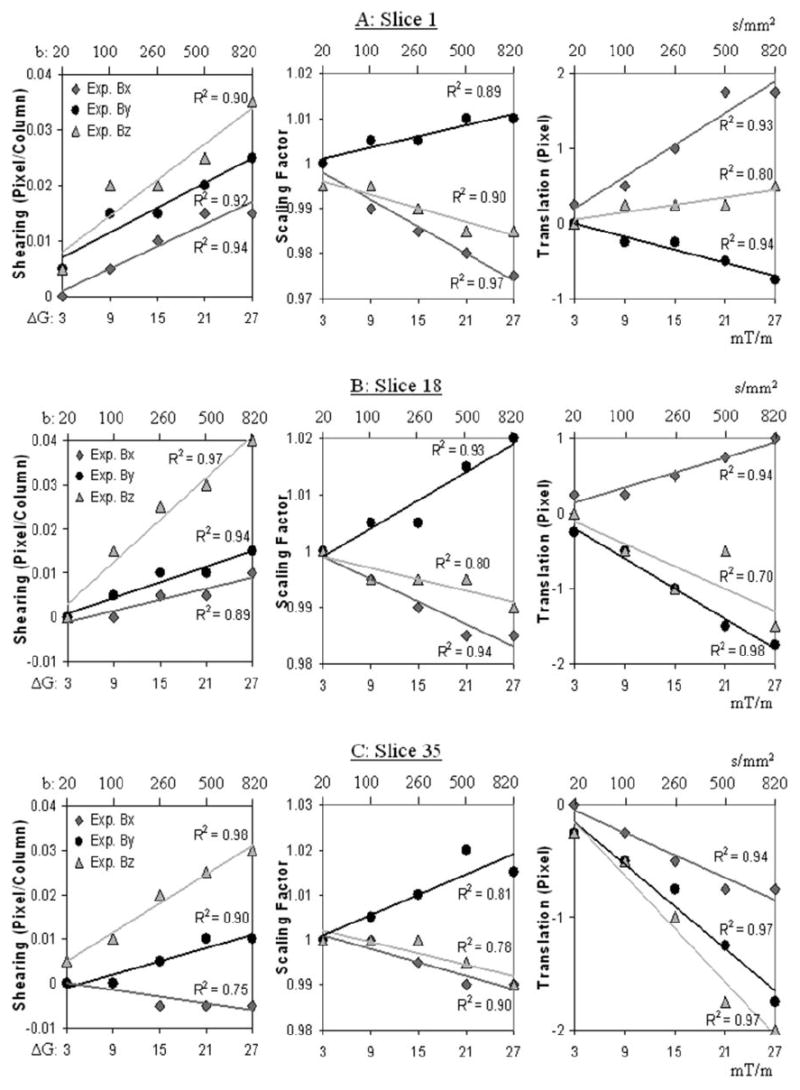
The parameters for each component of eddy-current distortion at slices 1, 18, and 35 vary linearly with the changed component of the diffusion gradients (presented in b-value on the top x-axis, and in gradient strength on the bottom x-axis), as described in experiment 2 and schemes B_x, B_y, and B_z of Table 1.

In experiment 3 we calculated the values of the eddy-current distortions relative to the non-DW images using our modeling method, and compared them with the corresponding values calculated by Haselgrove and Moore’s (8) algorithm. The values from the two methods were in close agreement across all gradient directions (Fig. 2), further supporting the validity and accuracy of the proposed algorithm.

Figure 2.

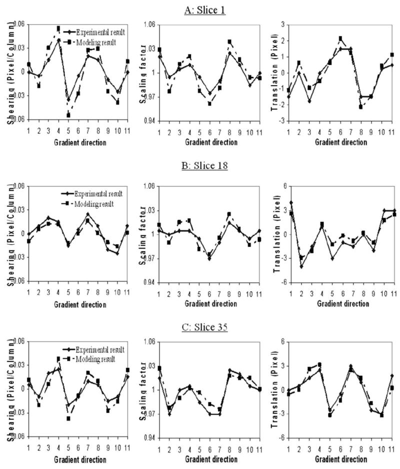
In experiment 3, the three components of distortion (shear, scaling, and translation) calculated by the proposed modeling algorithm (dashed lines) agree well with the distortions measured by Haselgrove and Moore’s (8) method (solid lines) on the experimental phantom data at slices 1, 18, and 35.

In experiment 4, tensor maps of human brains after correction show smoother contours and reduced blurring at tissue boundaries compared with maps constructed without correction (Fig. 3a and b). The number of negative eigenvalues decreased significantly after the correction was applied (Table 2). In contrast, the correction using Haselgrove and Moore’s method did not result in a statistically significant improvement (Table 2). This result demonstrates the effectiveness of the proposed algorithm.

Figure 3.

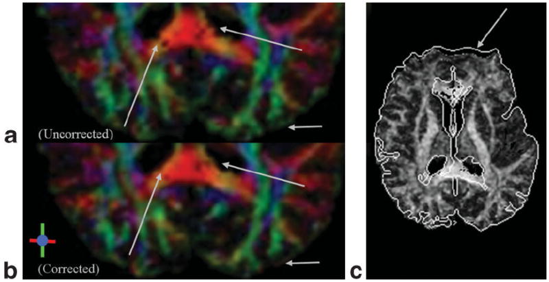
Representative DT maps constructed with and without prior application of the proposed algorithm at slice 18. a: The uncorrected tensor eigenvector map. b: The corrected tensor eigenvector map. The color bar at the bottom left is the color-coding scheme indicating the direction of the eigenvectors. The white arrows point to regions of significant improvement in the map. c: An FA map after distortion correction. The white contours outline the uncorrected FA map. The arrow indicates one obvious difference between the corrected and uncorrected maps.

Table 2.

Comparisons Between the Uncorrected Images, Images Corrected by Haselgrove’s Algorithm and Images Corrected by the Proposed Algorithm on Human Brains^*

Method	Mean	SD
Uncorrected	73.3	(22.7)
Haselgrove’s algorithm	71.9	(18.6)
Proposed algorithm	63.5	(19.4)
Comparison	t value	P value
Haselgrove’s algorithm vs. uncorrected	0.49	(>0.31)
Proposed algorithm vs. uncorrected	3.36	(<0.001)
Proposed algorithm vs. Haselgrove’s	3.20	(<0.001)

^*The table indicates the slice averages (mean) from 35 slices, standard deviations (SD), and t-tests (Comparison) for the number of pixels containing negative eigenvalues (described in Experiment 4 of human subjects).

The present results show that the various components of translation, shearing, and scaling in eddy-current distortions depend linearly on the corresponding diffusion gradient vector. Moreover, we have demonstrated that one can exploit this linear dependence to correct eddy-current distortions by using the known strength and direction of diffusion gradients that are applied to acquire the DW images.

Two previous attempts were made to model geometric distortions according to the gradient direction. One approach calibrated the distortion induced from the eddy currents for each of three orthogonal diffusion gradients in a phantom scan, and then applied these to ascertain the distortion in DW images acquired with arbitrary gradient amplitude and direction in a real human scan (9). However, the eddy-current distortion can depend on the detailed experimental conditions and scan parameters in each scan, such as RF coil, TE, slice orientation, and isocenter offset. It is difficult to calibrate this dependence in advance, but it can be modeled on a scan-by-scan basis in our current algorithm. Another recent approach used a mathematical framework to model geometric distortions according to slice position and gradient direction (16). However, the validity and practicality of that approach have not been demonstrated on either simulated or real DTI data.

The current linear model of distortions implicitly assumes that the time constants of significant eddy currents are long relative to the EPI readout to allow simple decomposition of eddy-current distortion into translation, shear, and scale. This may not be true if a different spectrometer or sequence is used. The model linearity should therefore be verified after such change is made, as well as after any adjustment of the time constants in the eddy-current compensation circuits.

In conclusion, the proposed method for correcting eddy-current distortions is both accurate and feasible in the real-world setting. The method not only circumvents the difficulties of prior correction algorithms that are associated with large differences in contrast across DW and non-DW images, it also eliminates the need to acquire additional images solely to aid in correcting distortion.

References

- 1.Basser PJ, Mattiello J, LeBihan D. Estimation of the effective self-diffusion tensor from the NMR spin echo. J Magn Reson B. 1994;103:247–254. doi: 10.1006/jmrb.1994.1037. [DOI] [PubMed] [Google Scholar]
- 2.Wider G, Dotsch V, Wuthrich K. Self-compensating pulsed magnetic-field gradients for short recovery times. J Magn Reson A. 1994;108:255–258. [Google Scholar]
- 3.Reese TG, Heid O, Weisskoff RM, Wedeen VJ. Reduction of eddy current-induced distortion in diffusion MRI using a twice-refocused spin echo. Magn Reson Med. 2003;49:177–182. doi: 10.1002/mrm.10308. [DOI] [PubMed] [Google Scholar]
- 4.Alexander AL, Tsuruda JS, Parker DL. Elimination of eddy current artifacts in diffusion-weighted echo-planar images: the use of bipolar gradients. Magn Reson Med. 1997;38:1016–1021. doi: 10.1002/mrm.1910380623. [DOI] [PubMed] [Google Scholar]
- 5.Jezzard P, Barnett AS, Pierpaoli C. Characterization of and correction for eddy current artifacts in echo planar diffusion imaging. Magn Reson Med. 1998;39:801–812. doi: 10.1002/mrm.1910390518. [DOI] [PubMed] [Google Scholar]
- 6.Calamante F, Porter DA, Gadian DG, Connelly A. Correction for eddy current induced B0 shifts in diffusion-weighted echo-planar imaging. Magn Reson Med. 1999;41:95–102. doi: 10.1002/(sici)1522-2594(199901)41:1<95::aid-mrm14>3.0.co;2-t. [DOI] [PubMed] [Google Scholar]
- 7.Papadakis NG, Smponias T, Berwick J, Mayhew JEW. k-Space correction of eddy-current-induced distortions in diffusion-weighted echo-planar imaging. Magn Reson Med. 2005;53:1103–1111. doi: 10.1002/mrm.20429. [DOI] [PubMed] [Google Scholar]
- 8.Haselgrove JC, Moore JR. Correction for distortion of echo-planar images used to calculate the apparent diffusion coefficient. Magn Reson Med. 1996;36:960–964. doi: 10.1002/mrm.1910360620. [DOI] [PubMed] [Google Scholar]
- 9.Horsfield MA. Mapping eddy current induced fileds for the correction of diffusion-weighted echo planar images. Magn Reson Imaging. 1999;17:1335–1345. doi: 10.1016/s0730-725x(99)00077-6. [DOI] [PubMed] [Google Scholar]
- 10.Bastin ME, Armitage PA. On the use of water phantom images to calibrate and correct eddy current induced artefacts in MR diffusion tensor imaging. Magn Reson Imaging. 2000;18:681–687. doi: 10.1016/s0730-725x(00)00158-2. [DOI] [PubMed] [Google Scholar]
- 11.Bodammer N, Kaufmann J, Kanowski M, Tempelmann C. Eddy current correction in diffusion-weighted imaging using pairs of images acquired with opposite diffusion gradient polarity. Magn Reson Med. 2004;51:188–193. doi: 10.1002/mrm.10690. [DOI] [PubMed] [Google Scholar]
- 12.Bastin ME. On the use of the FLAIR technique to improve the correction of eddy current induced artefacts in MR diffusion tensor imaging. Magn Reson Imaging. 2001;19:937–950. doi: 10.1016/s0730-725x(01)00427-1. [DOI] [PubMed] [Google Scholar]
- 13.Anderson E, Bai Z, Bischof C, et al. LAPACK users’ guide. 3. Philadelphia: Society for Industrial and Applied Mathematics; 1999. p. 407. [Google Scholar]
- 14.Basser PJ, Pierpaoli C. A simplified method to measure the diffusion tensor from seven MR images. Magn Reson Med. 1998;39:928–934. doi: 10.1002/mrm.1910390610. [DOI] [PubMed] [Google Scholar]
- 15.Bastin ME. Correction of eddy current-induced artefacts in diffusion tensor imaging using iterative cross-correlation. Magn Reson Imaging. 1999;17:1011–1024. doi: 10.1016/s0730-725x(99)00026-0. [DOI] [PubMed] [Google Scholar]
- 16.Andersson JLR, Skare S. A model-based method for retrospective correction of geometric distortions in DW EPI. Neuroimage. 2002;16:177–199. doi: 10.1006/nimg.2001.1039. [DOI] [PubMed] [Google Scholar]