Neural Correlates of Attention and Distractibility in the Lateral Intraparietal Area

Abstract

We examined the activity of neurons in the lateral intraparietal area (LIP) during a task in which we measured attention in the monkey, using an advantage in contrast sensitivity as our definition of attention. The animals planned a memory-guided saccade but made or canceled it depending on the orientation of a briefly flashed probe stimulus. We measured the monkeys’ contrast sensitivity by varying the contrast of the probe. Both subjects had better thresholds at the goal of the saccade than elsewhere. If a task-irrelevant distractor flashed elsewhere in the visual field, the attentional advantage transiently shifted to that site. The population response in LIP correlated with the allocation of attention; the attentional advantage lay at the location in the visual field whose representation in LIP had the greatest activity when the probe appeared. During a brief period in which there were two equally active regions in LIP, there was no attentional advantage at either location. This time, the crossing point, differed in the two animals, proving a strong correlation between the activity and behavior. The crossing point of each neuron depended on the relationship of three parameters: the visual response to the distractor, the saccade-related delay activity, and the rate of decay of the transient response to the distractor. Thus the time at which attention lingers on a distractor is set by the mechanism underlying these three biophysical properties. Finally, we showed that for a brief time LIP neurons showed a stronger response to signal canceling the planned saccade than to the confirmation signal.

INTRODUCTION

In everyday life, we are bombarded by a wealth of visual information. To manage this information, we focus our attention to objects or a specific region of visual space. Such attention is necessary for perception, learning, memory, and planning motor commands to interact with the world. In the monkey, neural correlates of visual attention have been seen in visual cortices (Li et al. 2004; Moran and Desimone 1985; Motter 1993; Reynolds et al. 2000; Treue and Maunsell 1999), posterior parietal cortex (Bushnell et al. 1981; Colby et al. 1996), prefrontal cortex (Everling et al. 2002), the superior colliculus (Dorris et al. 2002; Goldberg and Wurtz 1972; Robinson and Kertzman 1995), and the pulvinar nucleus of the thalamus (Petersen et al. 1985; Salzmann 1995). Generally, these studies have shown activity being modulated by attention. However, a growing number of studies have attempted to identify areas that may contribute to the allocation of visual attention by examining behavioral or physiological responses during microstimulation (Cutrell and Marrocco 2002; Moore and Fallah 2004) or reversible inactivation (Davidson and Marrocco 2000; Petersen et al. 1987; Wardak et al. 2004). These studies have shown that manipulations of posterior parietal cortex, the frontal eye fields, the superior colliculus, and the pulvinar nucleus of the thalamus can influence neuronal or behavioral measurements of attention. In this study, we focused on one of these areas, the lateral intraparietal area (LIP), whose neuronal responses are strongly modified by the behavioral relevance of the stimulus in the receptive field (Gottlieb et al. 1998; Toth and Assad 2002). Our aim was to correlate the activity from neurons in this area with a locus of attention measured behaviorally.

Attention can be defined in one of two ways: by showing enhanced sensitivity at an attended location (Bashinski and Bacharach 1980; Carrasco et al. 2000) or by measuring reaction times to visual events (Posner et al. 1980). We chose to define the locus of attention as the area of the visual field that has the best sensitivity to contrast. The benefit of measuring sensitivity is that it allows us to rule out the possibility that any advantage we see could be caused by influences in the motor system, a problem present when defining attention by changes in reaction time. Previous studies have shown that attentional benefits can be seen in the monkey both for changes in sensitivity (Ciaramitaro et al. 2001; Moore and Fallah 2001, 2004) and reaction time (Bowman et al. 1993; Witte et al. 1996).

Psychophysical experiments in humans have shown that attention is allocated to the endpoint of a planned saccade (Deubel and Schneider 1996; Shepherd et al. 1986) and that a flashed object (Egeth and Yantis 1997; Yantis and Jonides 1984, 1996) or a pop-out stimulus (Joseph and Optican 1996) can also attract attention. In this study, we used a modification of the memory-guided saccade task (Hikosaka and Wurtz 1983) to see whether attention is similarly modulated in the monkey and what the interactions were between exogenous and endogenous attention.

Some of the data presented here have appeared in brief form previously (Bisley and Goldberg 2003) and are appropriately labeled in the relevant figure legends.

METHODS

Subjects

All experiments were performed on two male macaque monkeys (Macaca mulatta) weighing ~ 9 and 10 kg, respectively. On weekdays, water was restricted before the experimental session, and the daily water ration was provided during the behavioral testing. On weekends, the monkeys were not tested behaviorally and received their water ration in their home cage. Food was continually available, and monkeys received supplements of fresh fruit daily. Body weights were recorded before every testing session to ensure good health and normal growth. The monkeys were implanted with scleral search coils and head restraint devices to monitor their eye position (Judge et al. 1980) and had recording cylinders placed above parietal cortex. All experimental protocols were approved by the NEI Animal Care and Use Committee as complying with the guidelines established in the Public Health Service Guide for the Care and Use of Laboratory Animals.

Surgical procedures

For all surgical procedures, which were performed under aseptic conditions, the animals were initially anesthetized with ketamine hydrochloride (15 mg/kg, im) and maintained with isofluorane through a closed rebreathing system. The concentration of isofluorane was varied from 1.5 to 3% depending on the animal’s pulse, blood pressure, and degree of relaxation. After all invasive surgical procedures, the animals were given a short course of cephalexin (250 mg twice a day for 3–5 days) and allowed to recover for 1–2 wk before returning to the laboratory. Custom-made titanium head pieces were attached to the skull using 9–12 titanium screws. Eye coils, made from fine wire (AS 632, Cooner Wire, Chatsworth, CA), were surgically implanted beneath the conjunctiva of each eye and were attached to plugs (SM2S, Powel Electrics, Philadelphia, PA) held onto the head piece by dental acrylic. Craniotomies were made over parietal cortex, and a recording cylinder was implanted. The chamber was 20 mm in diameter and was attached to the skull by a ring of bone cement anchored by six to eight plastic under-the-skull bolts. The cylinder was placed above the intraparietal sulcus, allowing a dorsal approach to LIP. The precise location and shape of the sulcus for each monkey was determined from MRIs obtained with a small surface coil in a 1.5-T G.E. Signa 2 scanner. For this procedure, the monkeys were lightly anesthetized with a mixture of intramuscular ketamine hydrochloride (10 mg/kg), atropine (0.4 mg/kg), diazepam (0.2 mg/kg), and butorphanol (0.05–0.1 mg/kg) and placed in a specially constructed MRI compatible stereotaxic frame.

Stimuli and behavioral testing

Behavioral control and data collection were done on computers using the REX system (Hays et al. 1982). Visual stimuli were back-projected on a tangent screen by a NEC Multisync LT100 DLP projector calibrated with a Tektronix J17 Photometer. The background luminance was 15 cd/m², and the projector refresh rate was 60 Hz. Stimulus timing was calculated by measuring a pulse from a photocell affixed to the back of the screen and illuminated by a small square on the corner of the same video frame as the appearance or disappearance of any stimulus. The monkey could not see the photocell or its illumination square.

The task was a variation of the memory-guided saccade task that allowed us to measure contrast thresholds (Fig. 1) and has been described briefly before (Bisley and Goldberg 2003; Bisley et al. 2004). The monkeys initiated a trial by fixating a small spot, and after a 1- to 2-s delay, a second spot (the saccade target) appeared for 100 ms at one of four positions equidistant from the fovea. The four positions changed from day to day but were constant on any given day. For the physiological studies, only two saccade target locations were used; one in the center of the receptive field (RF) and one opposite the center of the RF. At some time after the saccade target disappeared, a Landolt ring (the probe) and three complete rings of identical luminance flashed for one video frame (~ 17 ms), with one ring at each of the four possible saccade target locations. The animals had to indicate the orientation of the Landolt ring by either maintaining fixation (when the gap was on the right, a nogo trial) or making a saccade (when the gap was on the left, a go trial) after the fixation point disappeared. There was a 500-ms delay between the probe and the disappearance of the fixation point, so that the animals had ample time to cancel the planned saccade (Hanes and Schall 1995). In one-half of the trials a task-irrelevant distractor appeared for 100 ms 600 ms after the onset of the saccade target. The distractor was identical in shape and luminance to the saccade target, and appeared either at the site of the saccade target (henceforth referred to as the saccade goal) or opposite it. The luminance of the rings varied methodically so that an equivalent number of trials began with each contrast level. We defined the contrast threshold as the contrast at which the animal could discriminate the orientation of the Landolt ring at the 75% correct level. The contrast of the fixation point, saccade target, and distractor was 55%. The saccade target and distractor were 0.2° in diameter, the rings were 0.2° thick and 2.2° in diameter, and the gap in the probe was 0.8°. All objects apart from the fixation spot were at 10° eccentricity for the psychophysics and ranged from 6° to 34° for the physiology depending on the location of the center of the RF of the cell being studied.

FIG. 1.

Behavioral task. The monkey initiated a trial by fixating a small spot, and after a short delay, a 2nd spot (saccade target) appeared for 100 ms at 1 of 4 possible positions. At some time after the saccade target disappeared, a Landolt ring (probe) and 3 complete rings of identical luminance to the probe flashed for 1 video frame (~ 17 ms) at the 4 possible saccade target positions; 500 ms after the probe appeared the fixation point disappeared, and the animal had to indicate the orientation of the Landolt ring by either maintaining fixation for 1,000 ms (nogo trial) or making a saccade to the goal and remaining there for 1,000 ms (go trial). The Landolt ring could appear at any of 4 positions. In one-half of the trials, a task-irrelevant distractor, identical to saccade target, was flashed 500 ms after the target either at or opposite the saccade goal.

During fixation, animals had to keep within a 4° window, and they had 500 ms after the disappearance of the fixation spot to make a saccade to the remembered location of the saccade target or to maintain fixation within a 8° window in the center of the screen to receive a drop of water as a reward. When the animal was in the correct window for 500 ms, a spot appeared to reinforce the choice and to ensure that the animal did not drift out of the window in the remaining 500 ms. A psychophysics session consisted of 1,500–2,000 trials in which the four possible saccade target locations remained constant. We tested two stimulus-onset asynchronies (SOAs) in a session, and the proportion of trial types was 50% no distractor, 40% distractor opposite the saccade target location, and 10% distractor at the target location. In all trial types, the probe was placed at or away from the saccade target location with equal probability. In all the physiology trial types and in the psychophysics trial types with a distractor, there were two possible probe locations; in the psychophysics sessions performed before recording, there were four possible probe locations in trial types without a distractor. In this case, the probe appeared at the three nontarget locations in 16.5% of trials. The difference in probability did not have a major effect on performance—thresholds at the target locations were similar whether there were three or one other possible probe locations. We did not analyze data from the trials in which the distractor was flashed at the saccade goal because of the small sets of data collected within a single session. We included this trial type only to add uncertainty to the possible location of the distractor. We fitted data from the remaining trial types with Weibull functions, weighted by the number of trials at each point, using the maximum likelihood method (Quick 1974). The Weibull function was of the form

$$W(x)=0.5+(\gamma -0.5)(1-2^{-(\text{x}/\alpha )\beta })$$

where x was contrast; α was the centering parameter of the function; β was the steepness parameter of the function, 0.5 was the asymptotic minimum, and γ was the asymptotic maximum of the function. We defined the thresholds as the stimulus value corresponding to 75% correct.

We counted trials in which the animal broke fixation before the fixation point disappeared as fixation breaks, whereas we counted trials in which the monkey failed to make an appropriate saccade or failed to hold fixation in a nogo trial as errors. Therefore, although this is not a true two-alternative forced choice paradigm (i.e., the monkey could make an incorrect saccade on a go trial, which would still be counted as an error), we found that, below threshold, the animals ran at ~ 50% correct (data described in RESULTS). This enabled us to limit the lower asymptote of the Weibull function to 50%. When we fitted the data with a Weibull function that had the lower asymptote as a free variable, the pattern of significant differences in thresholds was conserved.

Both monkeys’ performances tended to vary slightly from day to day, so to visualize the data collected on different days, we normalized it on a daily basis to the monkey’s performance on trials in which there was no distractor and the probe was not at the location of the saccade goal. We always confirmed statistical significance using the raw nonnormalized data and excluded an individual day’s data from analysis when the nonnormalized threshold was > 3 SDs from the mean calculated with that point included. This resulted in the removal of only 11 thresholds from the 732 thresholds collected.

Electrophysiological recordings

We recorded single-unit activity through tungsten microelectrodes (1.5–5.0 MΩ; FHC). We inserted the electrode through a guide tube positioned in a grid (Crist et al. 1988). Neurons were identified as being in LIP based on their responses during a memory guided saccade and their location within the intraparietal sulcus (Barash et al. 1991). In this study, we recorded from every LIP neuron with visual activity that we encountered. Once we identified a neuron and isolated it well, we carefully mapped the position and size of its receptive field using a memory-guided saccade task, controlling saccade target position by joystick.

Data analysis

We discriminated action potentials during the trial using a BAK Dual Window Discriminator, and pulses were time stamped and stored together with information about the current stimulus in REX. We only used well-isolated single units for analysis.

In the physiology experiments, a spike-density function (Richmond et al. 1987) was calculated for each trial by convolving the spike train, sampled at 1 kHz, with a Gaussian with a sigma of 10 ms. Neuronal responses were shown as the average of this spike density trace over the interval of interest, across all common correct trials. To create the population data, we normalized each spike density function in the following way. First, we took the square root of every data point from all the functions for that cell. We divided each value by the total mean of the square rooted values from all the functions. We also normalized by dividing the raw activity by the raw mean or by using the maximal firing rate as normalizing factor. We also summed the data rather than normalize. Each method gave a similar temporal pattern of activity. For quantitative analyses we compared neuronal responses by calculating the number of action potentials over a 100-ms epoch from different trial types. For single cells we used a t-test to compare the data statistically, and Wilcoxon signed rank tests were used for the population comparisons. All data analysis programs were written in Matlab (Mathworks, Natwick, MA) using its curve-fitting and statistical capabilities.

CROSSING POINT ANALYSIS

We were interested in calculating the “crossing point,” the time at which the transient response to the task-irrelevant distractor fell below the level of delay period activity at the saccade goal. To determine the crossing point, we calculated the spike density functions from the cell or population using a sigma of 30 ms. In the cases in which there was more than one crossing point, we took the mean (and range) of all of the points on the functions that crossed between 100 and 700 ms after the distractor onset.

To see whether smaller populations of LIP neurons gave results similar to our complete population, we ran a shuffle analysis in which a limited number of neurons contributed to the population for each animal. In this analysis, the spike density functions created from these subpopulations were normalized and pooled, and the crossing point was calculated. This was repeated 2,000 times, providing us with a distribution of crossing points, each from a subpopulation of the neurons recorded.

DECAY OF ACTIVITY ANALYSIS

To show a relationship between the relative level of delay activity and the decay of the visual response, we fit an exponential function using Matlab’s lsqcurvefit function to the spike density functions smoothed with a sigma of 30 ms. We started our decay fit of the distractor response at the highest point of the spike density function after a minimum of the cell’s latency plus 20 ms. We have previously shown that LIP neurons have a highly synchronous initial response that creates an apparent biphasic peak (Bisley et al. 2004), so by starting the fit after the first peak, we got a much more appropriate function. In one-half of the trials, the probe appeared 700 ms after the distractor onset, so we fit the decay over a 500-ms epoch. For the main analysis presented here, we fit the response after the distractor with an exponential function that decayed to zero, although we also used asymptotic levels equal to baseline or left as a free parameter.

CALCULATION OF POPULATION RESPONSE SEPARATION TIME

We used a receiver operating characteristic (ROC)–based analysis (Bradley et al. 1987; Britten et al. 1992; Cohn et al. 1975; Green and Swets 1966; Tolhurst et al. 1983) to identify the time at which the activity from the population of neurons separated after the onset of the cue in different trial types. This analysis computes the time that an ideal observer could determine that the two trial types were different based on the distribution of responses. We performed the analysis on the normalized population response. At each millisecond of the function, we included the normalized responses from every trial from every cell. For each comparison, the responses at each ms in each function were compared by setting 62 evenly spaced threshold levels that covered the complete range of responses. For each level, the proportion of responses that were greater than the threshold was calculated for each distribution. The proportions for each distribution were plotted against each other to create an ROC curve. The area under this curve (aROC) gives the probability that an ideal observer could differentiate between the traces. An aROC of 0.5 indicates no difference in the distributions. A value of 0 or 1 indicates that the ideal observer could always tell which trial type the responses came from.

We ran a permutation test to calculate whether the aROC values were significantly different from 0.5. This was done by randomly distributing all the responses from both functions in a given 1-ms bin into two groups that were composed of the same number of data entries as in the original two distributions. We performed the same ROC analysis on the redistributed data and repeated this procedure 2,000 times, creating a distribution of aROCs. We determined where in this distribution the actual aROC lay (P value). We defined the time of separation as the first of ≥ 100 bins (of 1 ms) in which all the aROCs had a P ≤ 0.01.

RESULTS

Performance on the behavioral task

In each session, the monkeys were run on the task with six contrast levels, four possible saccade target locations, six trial types, and two SOAs. The trial types were probe at saccade goal; probe away from saccade goal; probe and distractor at saccade goal; probe and distractor opposite saccade goal; probe at saccade goal and distractor opposite; and distractor at saccade goal and probe opposite.

TRIALS WITHOUT A DISTRACTOR

When no distractor appeared, the monkey’s performance at the saccade goal was better than his performance away from the saccade goal. This is shown in Figure 2, which shows the monkey’s performance in all the trials in a single session in which no distractor appeared. Figure 2A shows the monkey’s performance when the probe was at the saccade goal. The squares show the percent correct at the six contrast levels from data pooled across saccade target locations. The solid line is the Weibull best fit, and the dotted line shows the threshold at 75% correct. Performance when the probe appeared away from the saccade goal is shown in Fig. 2B. In this example, we pooled the data from trials with all four saccade target locations and with the probe appearing at any of the three nontarget locations.

FIG. 2.

Psychometric functions from a single session from 1 monkey. A: trials in which the probe appeared at the saccade goal. B: trials in which the probe appeared at 1 of the 3 other locations that were away from the saccade goal. In both cases, data from saccade target locations in all 4 locations were pooled. Solid lines show best fitting Weibull functions. We defined contrast threshold to be the 75% correct level, indicated by dotted lines.

Performances at the three nontarget locations were similar (P > 0.2, Wilcoxon signed rank tests for all combinations within each animal across all prephysiology sessions). Mean thresholds were 1.73 ± 0.11 (SE), 1.73 ± 0.14, and 1.60 ± 0.07% contrast in monkey B and 3.27 ± 0.52, 3.24 ± 0.53, and 2.82 ± 0.20% contrast in monkey I. Each monkey showed a nonsignificant trend of better performance opposite the saccade goal. This was the location where the probe was more likely to appear throughout the session because it did not appear in the adjacent locations in trials with a distractor. Because these performances were not significantly different, we continued pooling the data from all three locations for all further analyses.

Contrast thresholds were lower in trials in which the probe appeared at the saccade goal than in trials in which the probe was elsewhere. Considering that the performance at the three nontarget locations was the same, these data suggest that the monkey was better at performing the discrimination when the probe appeared at the saccade goal. We suggest that this improved performance represents an attentional benefit at the locus of the saccade goal. To test this, we compared the thresholds from the two task conditions across all the sessions for each monkey. We found that the mean thresholds were significantly less at the saccade goal for all three SOAs (P < 0.05, Wilcoxon signed rank test), suggesting that there is an attentional advantage at the goal of the memory guided saccade for ≤ 1,800 ms after the saccade target flashes (Fig. 3, A and C). We normalized the thresholds for each SOA in each session using the performance at the nontarget locations (e.g., in Fig. 2, we divided the threshold from Fig. 2A by the threshold in Fig. 2B). In this form, an attentional benefit occurs when the data lie significantly beneath the dashed line, which represents the normalized contrast threshold at the nontarget locations.

FIG. 3.

Normalized contrast thresholds. A and C: normalized contrast thresholds taken at 3 stimulus onset asynchronies (SOAs) after the saccade target was shown for both monkeys. All points show significant attentional enhancement. B and D: normalized contrast threshold taken at 3 SOAs after distractor onset either at the saccade goal (blue) or distractor location (red) is shown for both monkeys. *Data that show significant attentional enhancement. In all plots, dashed line represents normalizing factor; points beneath the line indicate an attentional advantage. Modified from Bisley and Goldberg (2003).

To see whether this advantage manifested itself in forms other than the threshold, we also compared the slopes and upper asymptotes from these two trial types. We found that, for monkey B, the mean asymptotic performances were 95.5 ± 0.8 and 94.0 ± 0.8% correct for trials in which the probe was at and opposite the saccade goal, respectively (P > 0.1, Wilcoxon signed rank test). For monkey I, the mean asymptotic performances were 90.7 ± 1.2 and 90.0 ± 1.1% correct for trials in which the probe was at and opposite the saccade goal, respectively (P > 0.6). Similarly, the slopes of the functions were not significantly different (P > 0.2), with means of 4.37 ± 2.18 and 4.67 ± 2.10 for monkey B and 6.62 ± 2.46 and 10.58 ± 3.85 for monkey I, respectively. The large variances in these data come from a small number of poor fits that had very steep slopes (< 10% of all fits). However, the results did not change if these data were taken out (P > 0.2), giving mean slopes of 2.22 ± 0.34 and 2.59 ± 0.28 for monkey B and 2.37 ± 0.43 and 2.34 ± 0.32 for monkey I. Thus it appears that the attentional benefit was manifest as a lateral shift in the psychometric function. It is noteworthy that this is the result predicted by the neurometric functions calculated from the responses of V4 neurons in attended and nonattended locations (Reynolds et al. 2000).

TRIALS WITH A DISTRACTOR OPPOSITE THE SACCADE GOAL

Although attention usually lay at the goal of the memory-guided saccade, the sudden appearance of a distractor in the opposite hemifield transiently drew the animals’ attention. Figure 3, B and D, shows pooled normalized thresholds from trials in which the distractor appeared opposite the saccade goal. In these plots, the blue traces represent thresholds at the saccade goal and the red traces represent thresholds at the location where the distractor had flashed. Prenormalized thresholds that were significantly different from the normalizing thresholds (i.e., thresholds from trials with no distractor in which the probe appeared away from the saccade goal) are marked by the color-coded * (P < 0.05, Wilcoxon signed rank tests). In both monkeys, there was an attentional advantage at the distractor site 200 ms after the distractor, but not at the saccade goal. However, by 700 ms after the onset of the distractor, the attentional advantage had returned to the saccade goal and was no longer present at the distractor site. This suggests that there is a discrete locus of an attentional advantage that stays at the goal of a memory-guided saccade either until the monkey makes the saccade or until a distractor appears away from the goal. In this case, the locus of the attentional advantage briefly moves to the distractor site but within 700 ms moves back to the goal of the saccade.

Performance errors

The monkeys made five different types of errors during the trials. Two error types were simply consistent with the monkey’s misinterpreting the probe: type 1, continuing to fixate on go trials; type 2, making a saccade to the saccade goal on nogo trials. The other three were trials in which the monkey made a wrongly targeted saccade, errors that could occur whether or not the monkey misinterpreted the probe: type 3, making a saccade to the distractor on go trials; type 4, making a saccade that did not land near the goal or distractor site on go trials; type 5, making a saccade that did not land near the goal or distractor site on nogo trials. The number of times the monkey made each of these types of error is plotted for each probe contrast and for each monkey in Fig. 4, A and C. In Fig. 4, B and D, these data are shown as a proportion of the total number of error trials for each contrast. Both monkeys made more errors as the contrast decreased and the task became more difficult. As the contrast neared threshold the monkeys’ errors were predominantly making the wrong interpretation of the probe—either not making a saccade on a go trial or making the planned saccade on a nogo trial (classes 1 or 2). These data suggest that the animal was performing the task as a true two-alternative forced choice task. This is consistent with their chance performance at the lowest contrast, which was 51.6% correct for monkey B and 54.2% correct for monkey I.

FIG. 4.

Distribution of errors in the psychophysics. Numbers and relative proportions of error trials are plotted as a function of probe luminance and error type for each monkey. Bright columns represent high-contrast stimuli and dark columns represent low-contrast stimuli. Missed saccades are saccades that were made but landed > 5° from the saccade goal or the distractor site.

At suprathreshold contrasts, the monkeys made a small number of errors, but a greater proportion of these were not necessarily caused by misinterpretation of the probe (Fig. 4, B and D): making a saccade to the distractor on trials in which the monkey should have made a saccade to the goal (class 3) and making saccades that missed the saccade goal by > 5° on go trials (class 4). It is important to note that, in both monkeys, the absolute number of these nonmisinterpretation errors decreased as the task difficulty increased, suggesting that the monkeys may have been lulled into a deficit in general arousal or motivation after the suprathreshold probe appeared on easy trials. Monkey I also made a small number of errant saccades away from the saccade goal on nogo trials (class 5). These errant saccades were almost always downward saccades, independent of the saccade goal, and were equally likely across all probe contrasts. The dimensions of these saccades resembled those that caused fixation breaks in the early parts of trial and were likely to be fixation breaks occurring in the later parts of the trial.

Activity of LIP neurons during the task

We recorded 41 neurons in the same two monkeys that performed the psychophysical experiments described above. We selected neurons for analysis if they had a visual response to the saccade target of a memory-guided saccade; 34/41 (83%) of these neurons had delay period activity (P < 0.05, t-test; 600–1,200 ms after saccade target onset) and 32/41 (78%) had perisaccadic activity (P < 0.05, t-test; 100-ms epoch centered on saccade onset). RFs ranged from 6° eccentricity to 34° eccentricity. Response latencies to the saccade target ranged from 42 to 76 ms (for details, see Bisley et al. 2004).

In keeping with previous studies, LIP neurons responded to the onset of the saccade targets and often maintained activity during the delay period. They also responded to the abrupt onset of a distractor in the RF when the monkeys were planning a saccade elsewhere. Figure 5 shows poststimulus time histograms (20-ms bins) of the responses of three example LIP neurons during two trial types: when the saccade target was flashed in the RF and the distractor was flashed opposite the RF (left plots) and when the distractor, but not the saccade target, was flashed in the RF (right plots). The presentation times of the saccade target (T), distractor (D), and probe (P) are indicated by the horizontal bars beneath the abscissa. Each neuron showed a visual burst to the saccade target, some degree of delay activity, and a second burst to the probe (we show trials with the same probe appearance delay to prevent averaging of probe responses across different SOAs). We also pooled trials in which either a Landolt ring or the complete ring appeared in the RF.

FIG. 5.

Responses of 3 example lateral intraparietal area (LIP) neurons. Raster and poststimulus time histogram plots (20-ms bins) from trials in which the saccade target (T), but not the distractor (D), appeared within the receptive filed (RF; left) and from trials in which the distractor, but not the saccade target, appeared within the RF (right). In the raster plot, each line represents an action potential, each row a trial, and successive trials are synchronized on onset of the saccade target. Data are taken from trials with a common probe presentation time (P).

To categorize the neurons in terms of their visual and delay response, we calculated a visual/delay ratio in which the response 90–120 ms after the onset of the saccade target was divided by the response 600–1,200 ms after the onset of the target in trials in which no distractor appeared. The visual/delay ratios ranged from 1.38 to 9.17 and were 1.60, 2.39, and 4.31 for the example neurons in Fig. 5, A, B, and C, respectively. We recognize that some neurons in LIP show delay activity that changes over time (Fig. 5C, left plot); however, we feel that this ratio creates a reasonable categorization that can be used to differentiate neurons in LIP based on their response properties.

The population average response resembled the illustrated cells. Figure 6 compares the population responses from trials in which the saccade target, but not the distractor, appeared in the RF (blue traces) with the responses from trials in which the distractor, but not the saccade target, appeared in the RF (red traces). In both monkeys, there was a clear visual response to the appearance of the saccade target, distractor, and probe when they appeared in the RF. In both monkeys, there was clear delay activity in the population and the level of this activity was dependent on whether the saccade target appeared in the RF. This is most evident in the delay before the appearance of the distractor in which the blue traces are much higher than the red traces.

FIG. 6.

Normalized population responses from each monkey. Mean normalized population responses from trials in which the saccade target, but not the distractor, appeared within the RF are shown in blue and from trials in which the distractor, but not the target, appeared within the RF are shown in red. Data are taken from trials with a common probe presentation time. Eighteen neurons contributed to the population in monkey B and 23 neurons for monkey I.

In general, the population activity within the RF was unaffected by events outside the receptive field (Powell and Goldberg 2000). The one exception was that, in monkey I, the delay activity after the saccade target (blue trace) appeared to dip after the distractor appeared outside the RF. To see whether this represented a significant drop in activity, we compared the response in trials in which the distractor appeared away from the RF to that obtained from trials in which the saccade target appeared in the RF, but no distractor appeared (Fig. 7, green traces). In monkey B, the distractor had no effect on the delay response (Fig. 7A); however, in monkey I, the blue and green traces diverged slightly (Fig. 7B). The divergence occurred ~ 200 ms after the onset of the distractor and appeared to be caused by an increase in response of the delay activity rather than a suppression of the delay period activity by the distractor. These data were confirmed by plotting the responses during the epochs 0–200 and 300–500 ms after distractor onset against the same time (relative to saccade target onset) in trials in which no distractor flashed for the individual cells (Fig. 7, C and D). During both epochs, monkey B’s data were not significantly different (○; P > 0.1, Wilcoxon signed rank test), but monkey I showed significantly more activity 300–500 ms after the distractor onset than the no distractor control (●; P ≪ 0.001).

FIG. 7.

Delay response at a remote location does not drop when a distractor appears elsewhere. A and B: normalized responses from trials in which the saccade target, but not the distractor, appeared in the RF (blue traces), from trials in which there was no distractor and the target appeared in the RF (green traces), and from trials in which the distractor, but not the target, appeared in the RF (red traces). C: responses 0–200 ms after the distractor when the saccade target, but not the distractor, appeared in the RF are plotted against responses 600–800 ms after the saccade target (equivalent to 0–200 ms after the distractor) when no distractor was flashed and the saccade target was in the RF. D: responses 300–500 ms after the distractor when the saccade target, but not the distractor, appeared in the RF are plotted against responses 900–1,100 ms after the saccade target (equivalent to 300–500 ms after the distractor) when no distractor was flashed and the saccade target was in the RF. ○, data from monkey B; ●, data from monkey I. Some of these data have been presented previously as supplementary information in Bisley and Goldberg (2003).

Comparing the psychophysical data with the responses of neurons in LIP

The time-course of population activity in LIP correlated with the time-course of psychophysical performance. In dealing with the population responses, it can be easier to think of the responses from the two trial types in Fig. 6 as representing two populations of neurons with similar properties—one at the location where the saccade target was flashed (blue traces) and one at the location where the distractor was flashed (red traces). Thus we can think of these two traces as representing the responses at two locations on a salience map (Koch and Ullman 1985). Now if we compare the behavioral data in Fig. 3 with the normalized population responses of Fig. 6, we see a simple correlation. Whenever the blue trace (saccade target in RF) was higher than the red trace (distractor in RF), there was also an attentional benefit at the saccade goal. This was true 700 and 1,200 ms after the distractor was flashed and was true in trials in which no distractor was flashed—the population delay activity after the saccade target was always greater than baseline. Conversely, when the red trace was higher than the blue trace (immediately after the distractor flashed), an attentional benefit was present at the distractor location. This comparison is shown in Fig. 8, which shows both the psychophysical data (triangles) and the normalized population responses (bottom traces) for each monkey.

FIG. 8.

Pooled behavioral and neurophysiological data. Top: behavioral performance of the monkeys when the probe appeared at the saccade target (blue points) or distractor (red points) location in trials in which the saccade target and distractor were in opposite locations. Points that are significantly below dashed line show an attentional advantage at that site (color coded * show P < 0.05 significance tested with Wilcoxon signed rank tests). Triangles are results collected before recording from LIP neurons, and circles are results collected after. Lines in the bottom are mean normalized spike density functions from a population of 18 and 23 neurons for monkeys B and I, respectively. Spike densities are shown for all trials in which the probe appeared 700 ms or later than the distractor, but traces are cut off at 700 ms so as not to exhibit response to probe. Gray columns represent time during which activity in the 2 traces was not different—window of neuronal ambiguity. This is a modified figure from Bisley and Goldberg (2003).

These data suggest that the location with the greater activity is the location where attention will be allocated (Itti and Koch 2000). During the delay period, activity is greater at the goal of the memory-guided saccade, except when a distractor elsewhere evokes a transient response that rises above the delay period activity. This transient falls relatively quickly and soon crosses the delay period activity. For an epoch of 80 ms in each monkey, the two traces were not statistically significant (P > 0.05, Wilcoxon signed rank test on the activity of all the neurons over a 100-ms epoch measured every 5 ms), represented in Fig. 8 by the gray vertical column in each trace. We will refer to this time as the window of neuronal ambiguity. It spanned 415–495 ms in monkey B and 290–370 ms in monkey I. If attention is allocated to the spatial location evoking the greatest activity in LIP, we would predict that there should be no attentional advantage during this window. To test this, we stopped our recording sessions once we felt we had enough neurons to identify the window of neuronal ambiguity accurately and ran the monkeys on the psychophysics. We chose the time of the probe flash for each monkey to be in the middle of the window (455 ms for monkey B and 340 ms for monkey I) or 500 ms later (see APPENDIX A for an account of latency timing issues). Figure 8 shows these data (circles) together with the original psychophysical data (triangles), and the normalized population responses after the distractor onset.

The data points in the vertical gray bar show that, in both monkeys, there was no attentional benefit at either location during the window of neuronal ambiguity. However, there was an attentional benefit at the saccade goal during trials in which the probe was flashed 500 ms later, suggesting that the lack of benefit in the window of neuronal ambiguity is real. This supports the hypothesis that the locus of attention is related to the site of greatest activity in LIP.

We can further test this hypothesis, because the activity in the populations of neurons from the two different monkeys gave us sufficiently different windows of neuronal ambiguity. If the activity in LIP were really correlated with the behavior, at the time attention appears to be shifting in monkey B (455 ms), attention should have already shifted in monkey I, because the two neural response traces in Fig. 8B have completely diverged by this time. Conversely, in the middle of monkey I’s window of neuronal ambiguity (340 ms), the activity after the distractor is still significantly greater than the saccade goal delay activity in monkey B, so his attention should still be at the distractor site. We tested these hypotheses by presenting the probe to each monkey in the middle of the window for the other monkey. These data are included in Fig. 8 and confirm the predictions: in monkey B, the attentional benefit was still at the distractor site at 340 ms; and in monkey I, the attentional benefit was at the saccade goal at 455 ms.

Note that the absolute value of activity in LIP did not correlate with the locus of attention. Activity that was able to sustain the attentional advantage at the saccade goal could not do so when the distractor evoked much greater activity (1st 2 data points in Fig. 8A; 1st data point in Fig. 8B). The same psychophysical advantage occurred whether, as in the epoch of the distractor response, there was a huge difference between the activity at the distractor site and the activity at the saccade goal or when there was a small (but highly significant) advantage at the saccade goal as the distractor response decayed.

Controlling for task load

During the psychophysical experiments, the contrasts of the probe ranged from supra- to subthreshold, whereas during the majority of the physiological recordings, the probe had a constant suprathreshold contrast. Thus the task load was greater in the psychophysical experiments, and the monkey’s attentional allocation may have been different. Because the underlying premise of our hypothesis is that the population response in LIP at the time of the probe presentation is correlated with the attentional benefit, it is possible that the activity before the probe presentation may actually be different when the monkey is performing the more difficult task. To test for this, we examined the responses from four neurons (2 from each monkey) for which we had activity both during the basic physiological task and during the psychophysical task with all probe contrasts. Figure 9A shows the responses of the neurons during six 100-ms epochs (200 and 800 ms after saccade target onset in trials with no distractor and 200, 340, 455, and 650 ms after the distractor) as recorded in the simple physiological task and the more difficult psychophysical task. We have plotted the responses from both the trials in which the saccade target appeared in the RF and trials in which the distractor appeared in the RF. This gives us a total of 48 points, all of which lie close to the dashed line (representing equal activity in the 2 cases). Although the mean responses from the two tasks were significantly different (P < 0.05, Wilcoxon signed rank test), the mean difference was 2.3 spikes/s, and responses were slightly less in the task with higher load. Furthermore, there was a strong correlation between responses (R² = 0.90). Together these data suggest that, while there was a slight difference in response level during the two load levels, activity recorded in the suprathreshold task gives an excellent indication of activity during the psychophysical task in which the behavioral data were collected.

FIG. 9.

Neural responses and crossing points were similar in the full psychophysical task and in the suprathreshold task. A: responses of 4 neurons taken during 6 100-ms epochs (200 and 800 ms after saccade target onset in trials with no distractor and 200, 340, 455, and 650 ms after distractor onset) from trials in which the monkeys performed the full psychophysical task are plotted against the same epochs from trials in which the probe was always at suprathreshold contrast. We used the latter to collect physiological data from all neurons. B: crossing points calculated from smoothed data (30-ms sigma) from the full psychophysical task (the staircase session) for all 4 cells are plotted against the crossing points calculated from data from the suprathreshold session. For 1 neuron in 1 session, there were 2 crossing points, so we have plotted means and range of the 2 points.

The time-course of activity was also similar under the two task loads. We have already shown that the neuronal window of ambiguity can be used to predict when attention is shifting. To see if this was maintained under both task loads, we calculated for each condition the time at which the activity after the distractor decayed to the level of activity maintained at the saccade goal. In one case, the traces crossed twice; for this neuron, we calculated the mean as well as the range of crossing points. We compared the two crossing points from each neuron and found that they were similar (Fig. 9B). This analysis shows that not only were the levels of activity similar at different phases of the task, but that the time-course of the response profile was also maintained under high and low task loads.

Responses of single neurons in the population

Thus far, when discussing the responses of LIP neurons, we have only looked at the normalized population responses in the two monkeys. We will now show that the responses from single neurons have similar response properties to the population.

RESPONSES OF SINGLE NEURONS AT TIMES THAT PROBES APPEARED IN THE PSYCHOPHYSICAL TASK

We have already shown that the normalized population response of LIP neurons predicts where a monkey’s attention is in space. The activity of single neurons in this task reflects the population response. Figures 10 and 11 show the activity of single neurons during five epochs in which we measured contrast thresholds. The responses of neurons 750–850 ms after saccade target onset from trials in which the target did not appear in the RF are plotted against the responses from trials in which the target did appear in the RF in Fig. 10. The population activity was significantly stronger when the saccade target was in the RF than when it was out of the RF in both monkeys (P ≪ 0.001, Wilcoxon signed rank tests).

FIG. 10.

There was greater activity at the saccade goal than away from the saccade goal 750–850 ms after saccade target presentation. Responses from trials in which there was no distractor and the saccade target did not appear in the RF are plotted against responses from trials in which there was no distractor and the saccade target did appear in the RF for all neurons in both monkeys. This time is equivalent to the 1st SOA in Fig. 3, A and C.

FIG. 11.

Most neurons followed the response pattern seen in the population for each monkey. Responses from trials in which the distractor, but not the saccade target, appeared in the RF are plotted against responses from trials in which the saccade target, but not the distractor appeared in the RF at 4 epochs: 150–250 (A and B); 290–390 (C and D); 405–505 (E and F); and 600–700 ms (G and H). These times are equivalent to the 1st 4 SOAs in Fig. 8.

Likewise, whenever we found an attentional benefit after the distractor onset, it always corresponded with the location that had significantly more activity. In Fig. 11, A–C and F–H, the population responses all showed a significant difference in response between trials in which the saccade target, but not the distractor, appeared in the RF and trials in which the distractor, but not the target, appeared in the RF (P < 0.01, Wilcoxon signed rank tests), and this difference correlated with the locus of attention as shown in Fig. 8. However, during the window of neuronal ambiguity (Fig. 11, D and E), the population showed no difference in response and, as shown above, during this time there was no attentional benefit at either location.

For the most part, single cells had similar response profiles to the population. For instance, in all but one neuron, the response 800 ms into the delay was greater if the saccade target had appeared in the RF than if it had appeared elsewhere (Fig. 10), and these differences were significant in more than one-half of the neurons in each monkey (P < 0.0028 for monkey B, P < 0.0022 for monkey I, Bonferroni corrected t-test). Conversely, all but one neuron showed a greater response at the distractor site, 200 ms after the distractor, than at the saccade goal (Fig. 11, A and B), and these differences were also significant in more than one-half of the neurons in each monkey. As the response after the distractor waned, fewer neurons showed a significant difference in the conservative Bonferroni corrected t-test; however, in all of the epochs in which the population showed a significant difference, at least three neurons showed individual significant differences, and the difference was always in the same direction as the population difference. During the window of neuronal ambiguity, none of the neurons in monkey B (Fig. 11E) showed a significant difference. In monkey I (Fig. 11D), three neurons had significant differences during the window of neuronal ambiguity; however, the differences went both ways, with two neurons exhibiting more activity when the saccade target was in the RF and one neuron exhibiting more activity when the distractor was in the RF. In summary, we found that most of the neurons show the same pattern of activity as the population. Thus there is significantly more activity in single cells and the population as a whole at the saccade goal during a time at which we found a behavioral enhancement at that same location.

It is worth noting that, because the population activity in Figs. 6 and 8 contains neurons with both strong and weak delay activity, the difference in activity in the two traces is underplayed. Although the difference seen after the crossing point in Fig. 8A looks small, it is actually composed of a number of neurons that have firing rates that differ by 20–50 spikes/s during this epoch (Fig. 11G).

CROSSING POINTS FROM SINGLE NEURONS

The previous section suggests that individual neurons respond in a similar temporal manner during the task; however, we have already shown that neurons can have vastly different relative levels of visual and delay period activity (Fig. 5), with visual/delay ratios ranging from 1.38 to 9.17. To see whether neurons with different ratios do indeed follow the same temporal response characteristics during the trial, we calculated a metric, the crossing point, which represented the time it took for the activity after the distractor to decay to the level of activity maintained at the saccade goal and asked whether or not this metric was related to the visual/delay ratio.

We calculated the crossing point for each neuron by determining when the spike density function from trials in which the distractor appeared in the RF fell beneath the spike density function from trials in which the saccade target, but not the distractor, appeared in the RF (i.e., the time at which the red trace crosses to below the blue trace in Fig. 8). We limited crossing points by the minimum time at which the probe might appear (700 ms after distractor onset). To minimize the noise in the measurement, we used spike density functions smoothed with a 30 ms sigma. After this smoothing, only four neurons showed more than one crossing time. For these neurons, we defined the crossing point as the mean of all the times the activity after the distractor fell to less than the activity after the saccade target. In each case there were only two points, so we have plotted the range as well as the mean. One cell from monkey B showed no crossing point in this analysis; the response after the distractor fell to a level that was just above baseline, and the memory response 600–1,200 ms after the saccade target had already returned to baseline.

We found no clear relationship between the visual/delay ratio and the crossing point. The crossing points for each cell are plotted against their respective visual/delay ratios in Fig. 12. The gray bars show the window of neuronal ambiguity from the population data for each animal. The crossing points for individual cells are clustered near the window of neuronal ambiguity for each animal independent of the visual/delay ratio, and while there is some variance in the distribution of crossing points within the animals, there is little overlap between the two animals. Only five cells (28%) in monkey B had crossing points < 400, whereas only four cells (17%) in monkey I had crossing points > 400, and an ANOVA showed that the two means were significantly different (P < 0.02). This is important because the behavior predicted by this time was also different in the two animals (Fig. 8).

FIG. 12.

Crossing point for each neuron is plotted as a function of its visual/delay response ratio. For the 4 cells in which > 1 crossing point was calculated, we plot both mean and range of all the times that the activity after the distractor dropped below the activity after the saccade target. Closed symbols mark neurons with distractor activity that was well fit with an exponential function.

There was no linear correlation between the visual/delay ratio and crossing point in either monkey (monkey B: R² = 0.04, P = 0.20; monkey I: R² = 0.02, P = 0.24). This suggests that the decay in response after the distractor must be different for neurons with different visual/delay ratios, because if all the neurons had the same rate of decay, the activity would consistently cross earlier for neurons with low ratios (relatively more delay activity) and much later for neurons with high ratios (relatively less delay activity). Thus we predict that cells with low ratios should decay more slowly after the distractor, and cells with higher ratios should decay more rapidly.

This was in fact true: the crossing point was related more to the monkey than to the nature of the individual neurons in which it was measured. To show this, we first fit an exponential function to the decay in the response evoked by the appearance of the distractor. An example of such a fit is shown for a neuron with a visual/delay ratio of 3.6 in Fig. 13A. This neuron had the median R² for that animal (0.97) and gives a good indication of how well the responses were fitted by the exponential. For most of the neurons (13/18 in monkey B, 20/23 in monkey I), the exponential fits were very good with R² > 0.75. These neurons are represented by the filled symbols in Figs. 12–14. We chose not to use the remaining eight neurons in the analysis because the time constants calculated from these fits were not good enough approximations of the neural data and thus could have given misleading relationships between the ratio and the decay. However, neurons with good exponential fits covered the entire range of visual/delay ratios (Fig. 12) and, in fact, provided the upper and lower bounds for each sample. Thus by rejecting neurons with bad exponential fits we were not obviously discriminating against any particular range of visual/delay ratios.

FIG. 13.

For each animal, there is a relationship between visual/delay ratio and rate of decay of activity after the distractor. A: response, plotted as a spike density function, of a single neuron from trials in which the distractor (time marked by 2nd black bar), but not the saccade target (time marked by the 1st black bar), appeared in the RF. Third black bar indicates time of probe presentation in one-half of trials. Thin black line shows fitted exponential function (R² = 0.97). This was the median fit for this animal. B and C: log of visual/delay response ratio is plotted against decay rate constant from the exponential fit for neurons that had good fits (R² > 0.75; ●) and for neurons with poor fits (○). Solid black lines show linear functions fitted to data from neurons with good exponential fits. In this figure, visual response was calculated from peak of the fitted exponential and delay response (600–1,200 ms after saccade target onset) from trials in which the saccade target appeared in the RF and the distractor appeared out of the RF.

FIG. 14.

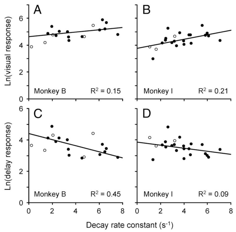
Log of visual and delay responses are individually plotted against rate of decay of activity after the distractor for each animal. ●, neurons with good exponential fits (R² > 0.75); ○, neurons with poor exponential fits. Linear functions were only fit to ●.

Figure 13, B and C, shows the natural log of the visual/delay ratio plotted against the decay rate constants of the exponential fits for all the cells. Neurons whose functions were fit well by the exponential are represented by the filled circles, and those that were not fit well are represented by the hollow circles. The black solid lines are linear fits through the solid symbols. We chose to plot the ratio as a log, because this means that the slope of the linear fit is the time from the peak of the exponential function to the crossing point (see APPENDIX B for details). However, because the visual/delay ratios calculated above (i.e., for Fig. 12) are based on the visual response to the saccade target and the memory activity in trials in which no distractor appeared, they are not appropriate for estimating the crossing point. Instead, in this figure we show visual/delay ratios calculated using the peak of the fitted function to the distractor response as the visual response and the delay activity at the site of the saccade goal from trials in which the saccade target appeared in the receptive field and the distractor appeared outside of the receptive field. We will show below that using the original visual/delay ratios does not change the results.

The estimated population crossing points, calculated from the slopes of the black lines, were 421 and 375 ms for monkeys B and I, respectively. These were both within the windows of neuronal ambiguity calculated from the population averages for each monkey and within 33 and 35 ms, respectively, of the times that we determined psychophysically that attention is shifting (Fig. 8). Note that with one exception, even the neurons that were not fit well by the exponential function (hollow circles) lay near to or within the population. The one exception from monkey I is not plotted because it lay well off the bounds of the axes.

The relationship we see between the visual/delay ratio and the decay rate of activity after the distractor was not caused by one of the two factors that make up the ratio. Figure 14 plots the ratio separated into its components against the decay rate constant for each monkey. The lines are fitted only to the solid circles, which again represent neurons that were well fit by the exponential function. In every case, the R² from the component analysis is well below that obtained from the ratio in Fig. 13. This suggests that the visual response, delay activity, and decay rate after the distractor co-vary in such a way as to keep the crossing point constant.

To test whether the relationship between the visual/delay ratio and the decay rate is robust, we changed three parameters independently and redid the analyses. In the first of these tests, we changed the smoothing factor used to create the spike density functions. Normally we present data using a sigma of 10 ms (see Fig. 6), but for calculating the crossing point we used a relatively broad sigma (30 ms) to reduce the bumpiness of the trace and thus provide a single crossing point for most cells. Changing the sigma made little difference, as shown in Fig. 15A, which compares the crossing points obtained by smoothing the traces with these two kernels. Although the traces crossed more often in the 10-ms data, the mean crossing points were not different (P > 0.5, Wilcoxon signed rank test), suggesting that the mean crossing point calculation does not depend on the level of smoothing. Similarly, using a 10 ms sigma had only a small effect on the fit of the delay ratios to the time constants (Fig. 15, B and C). Unsurprisingly, the mean R² for the exponential fits of the less smoothed data were not as high as for the more smoothed data (0.78 compared with 0.86), but the correlations between the ratio and decay rate were similar. Based on the linear fits to the neurons whose less smoothed data were fit well (R² > 0.75; solid points) the estimated crossing points were 438 and 366 ms for monkeys B and I, respectively, within 17 and 26 ms of the behaviorally confirmed crossing points, respectively. Thus the level of smoothing applied to the raw data did not affect the relationship between the visual/delay ratio and the decay rate.

FIG. 15.

Relationship between the decay rate constant and the log of the visual/delay ratio was robust. Plots in the left column compare alternative data sets to data presented in Fig. 13. Center and right columns show that even with the alternative data sets, relationship between the log of the visual/delay ratio and the decay rate constant was still fairly strong. ○, data that were not well fit (R² ≤ 0.75) by the exponential function. A–C: use of a sigma of 10 ms to convolve the spike data gave similar results to the sigma of 30 ms used in the main analysis. D–F: visual/delay ratio calculated from trials in which there was no distractor and the saccade target appeared in the RF (visual response: 90–120 ms, delay response: 600–1,200 ms) is compared with the ratio using the peak of the fitted exponential as the visual response and the delay response (600–1,200 ms after saccade target onset) from trials in which the saccade target appeared in the RF and the distractor appeared out of the RF. We used the former to categorize the neurons in Fig. 12, and the latter for the main analysis in Fig. 13. G–I: decay rate calculated by fitting the activity with an exponential whose asymptote was left as a free parameter is compared with decay rate calculated by fitting activity with an exponential that decayed to 0. We used the latter in the main analysis. G: hollow diamonds show data that, on visualization, clearly overestimated decay rate by dropping to threshold level before the activity trace did.

In the second of these reanalyses, we compared methods of calculating the visual/delay ratio. The two ratios in this comparison have been used before: one in Fig. 12 and the other in Fig. 13. We calculated the first ratio by dividing the visual response to the saccade target (90–120 ms after target onset) by the response 600–1,200 ms into the delay in trials in which no distractor ever appeared. We used this ratio to categorize LIP neurons (see Fig. 5 and related text) and in the analysis in Fig. 12. The second ratio came from the peak of the fit to the distractor response and the delay activity from trials in which the saccade target appeared in the RF and the distractor appeared opposite the RF. We used this ratio in the analyses in Figs. 13 and 14. The two different calculations of ratio are plotted against each other in Fig. 15D and are not significantly different across the population (P > 0.1, Wilcoxon signed rank test). We also plotted the log of the ratio taken from the saccade target response (and used in Fig. 12) against the decay rate constant from the original fits (using a sigma of 30 ms) and found that the correlations had not changed (Fig. 15, E and F).

We stated above that the estimated crossing point, taken from the slope of the linear fit through the solid points (i.e., the cells that had good exponential fits), would not be valid if we used the ratio from Fig. 12. There are two reasons for this: first, the original ratios were calculated with the visual response to the saccade target, not the distractor; second, the original memory response was taken from trials in which the distractor did not appear and we have already shown that in monkey I the response during this period is slightly different if the distractor appears (Fig. 7). Thus we expect that the estimated crossing point may be inaccurate. However, to show the robustness of the relationship between the ratio and decay rate, we estimated the crossing points anyway and found them to be 50 and 60 ms from the behaviorally confirmed crossing points in monkey B and I, respectively. Although these both lie just outside of the window of neuronal ambiguity, they are particularly close given the inherent inaccuracies expected using this ratio. We also ran this analysis using a number of different epochs (50–200, 50–150, 100–150 ms following either the saccade target or distractor) or using the peak of the exponential fit to the saccade target for the visual response. In each case, we obtained similar correlations. Thus we are confident that the correlation between the visual/delay ratio and the decay rate is robust to the epochs chosen to represent the visual and memory responses.

In the third reanalysis, we changed the parameters of the exponential fit so that the activity did not decay to 0, but reached an asymptotic level that was left as a free parameter. To maximize the time over which the asymptote was measured, we only used those trials in which the distractor probe SOA was 1,200 ms. This resulted in only one half of the trials contributing to the data. While this is a slightly more accurate representation of what the decay might look like over time, we chose not to do this in the main analysis for two reasons. The primary reason was that if we included an asymptotic level in our fit, we could not estimate the crossing point from the correlations in Fig. 13. The second reason was that since the original fit was over such a short period, the response was often still falling at a reasonably rapid rate (see Fig. 13A for example) and as such the fits were very good. This meant that the introduction of a third parameter barely improved the fits. The mean R² increased from 0.84 to 0.93 and the median R² increased from 0.93 to 0.96. When we included the free asymptote, the correlations between the visual/delay ratio and the decay rate were still fairly robust. Figure 15G shows the decay rate constants taken from the two and three parameter exponential fits plotted against each other. Three sets of cells are plotted: the neurons that were well fit by the exponential (R² > 0.75; ●); two neurons that were well fit by the exponential, but on visual inspection clearly overestimated the decay rate, by dropping to an asymptotic level well before the activity trace did (◇); and the neurons that despite the third parameter were still poorly fit by the exponential (R² < 0.75; ○). For neurons that were well fit by the exponential, there was a clear correlation (R² = 0.79, P ≪ 0.001; solid line); however, the mean rates were different (slope: 0.74; intercept: 3.4 s⁻¹). Despite this difference, there was still a reasonable correlation between the visual/delay ratio and the decay rates estimated with the three parameter fit (Fig. 15, H and I). Note that the poor fitting high rate estimates (> 10 s⁻¹), showed by the hollow circles and diamonds in Fig. 15G are not plotted in Fig. 15, H and I. As mentioned above, we cannot accurately derive an estimated crossing point from these data, because Eq. B3 of APPENDIX B would have an asymptotic shift parameter on both sides of the equation. However, if we assume that the shift is minimal, we can look at the slopes of the fits and get an approximation of the crossing points. In this case the estimated crossing points are within 144 and 43 ms of the behaviorally confirmed crossing points in monkey B and I, respectively. We have also performed this analysis when fitting the asymptote to the baseline level of the neuron (assuming that the decay after the distractor would approach baseline), and found results that were even more similar to the original data. Thus the relationship between the visual/delay ratio and the decay rate is robust—withstanding changes in smoothing, choice of epoch, and fitting parameters.

HOW MANY CELLS ARE NEEDED TO CALCULATE THE CROSSING POINT?

One question remains about the relationship between the visual/delay ratio and the decay rate of the distractor response: is this relationship useful for the monkey in this task?

One possible way that this consistency among neurons could be used by the monkey is in minimizing the number of neurons needed to create the salience map. To show this, we ran a series of simulations in which we limited the number of neurons that contribute to the population. Specifically, to create the population we randomly picked a small number of neurons (n) from a monkey, pooled the mean normalized responses from the same trial types, and calculated the crossing point. We repeated this 2,000 times for each n and compared the resulting distributions of crossing points to the window of neuronal ambiguity (i.e., the crossing point for the entire population). One can think of these data as coming from two populations neurons, one at the saccade goal and one at the distractor site, each of which has the exact same response properties. At the single neuron level, this is often referred to as a neuron anti-neuron pair. These data are shown in Fig. 16 for both monkeys. In the top plots (Fig. 16, A and B), we showed the mean and SD for each resulting distribution plotted as a number of the neurons that were pooled to create the distributions. The horizontal gray bars represent the windows of neuronal ambiguity. It is clear that even with only one neuron anti-neuron pair, the mean of the distribution is within the window of neuronal ambiguity, as expected based on the results shown in Fig. 12. However, what is more impressive is that the SD rapidly shrinks until it is well within the window.

FIG. 16.

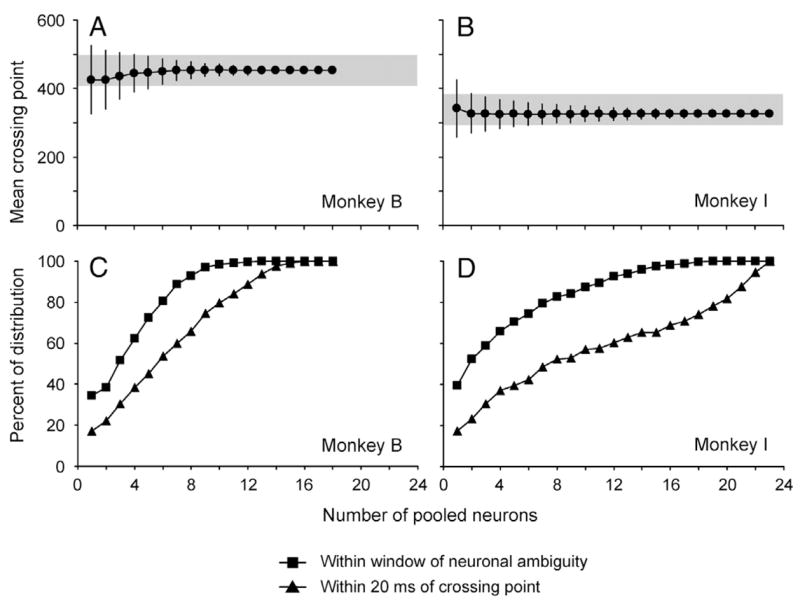
Very few neuron/anti-neuron pairs are needed to establish crossing point. A and B: mean ± SD crossing points from 2,000 iterations are plotted as a function of the number of neurons that were pooled to produce the crossing point. Gray bar represents window of neuronal ambiguity from the population. C and D: proportion of crossing points from 2,000 iterations that lie within the window of neuronal ambiguity (squares) and within 20 ms of the pooled crossing point (triangles) are plotted as a function of the number of neurons that were pooled to produce crossing point.

We can examine this more closely by plotting the proportion of the distribution that lies within the window of neuronal ambiguity as a function of number of neurons pooled (Fig. 16, C and D, squares). This proportion reaches 100% with only 12 neurons in monkey B and 18 neurons in monkey I. Furthermore, we find that the entire distribution made from 16 randomly picked neurons lies within 20 ms of the behaviorally defined crossing point in monkey B (Fig. 16C).

In the analyses presented in Fig. 16, we used all trials from each neuron in each neuron/anti-neuron pair. This technique washes out any noise that would be present in a single trial. To see if the analyses hold true with in a more realistic state, we ran the same simulation, but with every neuron contributing only one trial of data in each condition. We found that 43% of the simulated crossing points were within the window of neuronal ambiguity for monkey B (18 neurons contributing), giving a mean of 440 ms and an SD of 75 ms. Monkey I’s data were even more compelling with 64% of the crossing points lying with his window of ambiguity. Again, the mean of 329 ms was close to the population crossing point of 340 ms, and the SD of 45 ms reflects how tight the distribution was. The conclusion of these analyses is that if each neuron is paired with an anti-neuron with a similar visual/delay ratio (and thus a similar decay rate after the distractor), very few neurons are needed to create a consistent population response, even if each neuron only contributes one trial worth of data. We think it is highly unlikely that the brain uses only a small number of neuron anti-neuron pairs at any given time. Rather, we see this as an explanation of why we are able to show such consistent neuronal responses despite a small data set.

Activity of neurons in error trials

Errors in the physiological task, in which the probe was always supracontrast, made up < 10% of all trials. As in the psychophysics (Fig. 4), the majority of errors were made when the monkey did not make a saccade on a go trial (class 1). Unlike in the psychophysics experiments, however, the second most common error was to make a saccade to the distractor site on a go trial (class 3). While the proportion of these error trials was < 2.5%, it is important to note that this error could only be made on trials in which a go probe appeared and the distractor and saccade target appeared in opposite locations. This limited the number of trials in which this error could occur, such that the actual proportion of errors for this trial type was much higher (12.5%).

As we have already stated, to predict where an attentional benefit will be found in our task, we must look at the activity in LIP when the probe appears. To see if activity at this time could explain the errors, we compared the response in a 100-ms epoch just before the probe presentation on individual error trials to the mean activity from that epoch in the correct trials. On go trials in which the monkey made an erroneous saccade to the distractor instead of the saccade target (class 3 errors), the response at the saccade goal before probe presentation was significantly weaker than in the equivalent correct trials (P ≪ 0.01, Wilcoxon signed rank test) and significantly stronger at the distractor site in error trials than in correct trials (P ≪ 0.01). On go trials in which the monkey did not make a saccade (class 1 errors), the activity before the probe was slightly less than in trials in which he correctly made the saccade (P < 0.02, Wilcoxon signed rank test). On these types of error trials, the activity before the probe presentation was not different when the distractor or nothing was flashed in the RF (P > 0.05). Whether or not the probe itself was in the RF made no difference to these results. Together, these data suggest that rather than the errors being caused by attention being misdirected, it is most likely that the monkey was not performing the underlying task perfectly.

Responses to the probe stimuli

Until now we have focused on the responses of LIP neurons before the presentation of the probe. These data have established that activity in LIP at the time the probe appears determines the locus of attention as defined by the perceptual advantage for discrimination of the probe. In this section, we will examine the responses of LIP neurons after the onset of the probe.

The initial response to the probe did not identify the locus of attention, and only after 115 ms did it differentiate between probe identities. Figure 17 shows the normalized population responses from both monkeys to the go, nogo, and null probes presented in the RF in trials in which the saccade target appeared in or opposite the RF. The responses are aligned with the onset of the probe and include all SOAs. Note that the activity before probe appearance is consistent with the delay period activity in the delayed saccade task and predicts the locus of attention as measured by its discrimination. When the saccade plan was toward the RF of the neuron (blue and orange traces), the activity before probe appearance was greater than when the saccade plan was away from the RF (green and red traces). The probe evoked a transient response on every trial, because an object, either a circle (the null probe) or a Landolt ring (the go or nogo probe), appeared in the receptive field on every trial. The transient response to the probe onset was the same in all cases, but the nature of the decay of the transient response differed from case to case, depending on the nature of the probe signal and the location of the saccade goal. When the probe in the RF confirmed the saccade plan, the decay rate was rapid, falling to near the delay period level when the saccade goal was in the RF (thick blue traces) and to near the low baseline rate when the saccade goal was away from the RF (thick red traces). The decay rates when the null probe was in the RF on both go and nogo trials were similar to when the go probe was in the RF (all thin traces) and only the final level of activity depended on whether the saccade plan was toward (thin blue traces) or away from (thin orange, red and green traces) the RF. These data suggest that the activity of neurons in LIP represents the decision to go or not to go at the same time, irrespective of whether a go or null probe appears in the RF. We quantified the time that the thick red and blue traces diverged using an ROC analysis (see METHODS) and found that LIP neurons reflected the decision of where to go 212 and 185 ms after the probe onset for monkeys B and I, respectively.

FIG. 17.

Normalized population responses from each monkey to the go, nogo, and null probes under 4 task conditions. Thick black bar shows time of presentation of probe. Color coding indicates direction of saccade plan and whether the trial was a go or nogo trial, and thickness of the line indicates whether the probe was in the RF.

More surprisingly, however, when the nogo probe appeared in the RF, the decay rate was much slower, regardless of whether saccade was planned to the RF (thick orange trace) or away from it (thick green trace). This means that for a period of almost 150 ms there was more activity after the nogo probe than after the go probe, even when the monkey had received confirmation of a planned saccade into the RF. The two nogo response profiles separated from all the other profiles fairly soon after probe onset. Using an ROC analysis, we found that the separation between the combined nogo data (thick orange and green traces) and the combined go data (thick blue and red traces) occurred at 113 and 116 ms after the probe onset for monkeys B and I, respectively. This means that the probe discrimination occurs within ~ 115 ms, because at this time, LIP neurons differentiate between a go or nogo probe within their RF. It also means that, within this population of neurons, probe discrimination occurs 70–100 ms before the representation of the decision to make the saccade.

This response profile was typical of the population. For cases in which the saccade was planned to the RF, and the probe in the RF, there was no difference between go and nogo responses 0–100 ms after probe appearance (Fig. 18A; P > 0.05, Wilcoxon signed rank test). However, 150–250 ms after the probe appearance, there was a significantly greater response to the nogo probe than to the go probe (Fig. 18B, P < 0.001, Wilcoxon signed rank test). These are the data that contributed to the blue and orange traces in Fig. 17, and it is clear that, in all but 2 of the 41 neurons, the responses to the nogo probe were greater than or equal to the responses to the go probe.

FIG. 18.

Responses of single neurons after probe presentation. A: responses to the go and nogo probe are compared 0–100 ms after onset of the stimulus. B–F: responses 150–250 ms after probe onset are compared under 5 pairs of task conditions. Data from monkey B (○) and monkey I (●) are plotted separately.

When the monkey was planning a saccade to the RF, the response to the go probe in the interval 150–250 ms after probe appearance was not different from the response to the null probe when the go probe appeared elsewhere (Fig. 18C, P > 0.5). However, in the interval 150–250 ms after probe onset, the response to the nogo probe was enhanced across the population relative to the null probe when the nogo probe appeared outside of the RF and the monkey was planning a saccade into the RF (Fig. 18D, P < 0.001). This was true for 39 of 41 individual neurons. Therefore the enhancement in the nogo case is caused by the actual nogo stimulus appearing in the receptive field of the neuron, and not just the arousal caused by the monkey’s having to cancel the saccade to the RF.

The nogo enhancement did not require that the saccade goal lie in the RF, as long as the nogo probe was in the RF. Figure 18E plots the response to the nogo probe in the RF during trials in which the monkey planned a saccade away from the RF against the response to the same stimulus during trials in which the monkey planned a saccade to the RF. In monkey I, we found that the responses were not different in the two cases (●; P > 0.1, Wilcoxon signed rank test), suggesting that the nogo probe response is independent of saccade direction. However, there was a small, but significant, difference in monkey B (○; P < 0.01). This small difference, and a trend in this direction in monkey I, may represent the slight dampening of response in an attended location (i.e., the saccade goal) that has been previously documented in posterior parietal cortex (Constantinidis and Steinmetz 2001; Powell and Goldberg 2000; Robinson et al. 1995).

The final question we addressed was whether the nogo probe enhancement was entirely independent of the saccade plan. Figure 18F plots the responses to the nogo probe placed in the RF against the responses to the go probe placed in the RF from trials in which the saccade is planned away from the RF. Again, 39 of 41 neurons show greater activity to the nogo probe than to the go probe (P ≪ 0.001, Wilcoxon signed rank test), and this effect was even greater than when the saccade was planned to the RF (cf. Fig. 18, B and F).

DISCUSSION

In this study, we showed that a monkey’s attention, as measured by perceptual threshold, is pinned at the goal of a memory guided delayed saccade for the duration of the delay period, unless a task-irrelevant distractor appears elsewhere in the visual field. The activity of neurons in the LIP correlates with the monkey’s locus of attention in an extremely stable manner. Both the aggregate neuronal and single unit activity in LIP predicted when a given monkey’s attention would return from the distractor to the saccade goal in experiments we ran months after we recorded the neuronal data. We will discuss these results in terms of previous physiological and psychophysical results and propose a hypothesis of LIP’s function in the primate brain that explains its relationship to both visual attention and the generation of eye movements.

Psychophysics of attention

The finding that an attentional benefit lies at the goal of a memory-guided saccade is consistent with results from prior human psychophysical studies using visually guided saccades (Deubel and Schneider 1996; Kowler et al. 1995). In our hands, this benefit lasted for the duration of the trial, suggesting that attention is pinned to the goal of the saccade. However, recently Ostendorf et al. (2004), using accelerated manual reaction time as the measure of attention, found that attentional benefits were only seen during the first 300 ms of a memory-guided saccade, after which reaction time slowed. However, this result may be more related to the inhibitory mechanisms introduced by using manual reaction time as a measure of attention (Klein 2000; Posner and Cohen 1984; Posner et al. 1985) than to a failure of a saccade plan to guide attention during the delay period in humans. We have recently found that in the monkey manual reaction time is also slowed during most of the delay period of a memory-guided saccade, but this result was reversed when the manual reaction time trials were interleaved with the more difficult go/nogo trials described in this study (B. S. Krishna, S. C. Steenrod, J. W. Bisley, Y. B. Sirotin, and M. E. Goldberg, unpublished data). In that case, manual reaction times were accelerated throughout the delay period, consistent with the data presented here.

Our results are also in keeping with the general finding that the abrupt onset of a distractor draws attention (Egeth and Yantis 1997). In addition, we have shown that this effect is strong enough to draw attention away from a predefined locus of attention at the saccade goal. The surprising finding is that this effect never waned over months of study and hundreds of thousands of trials. The stability of the distractor response may be related to the fact the monkeys, unlike humans, cannot change the attentional advantage of a cue in a manual reaction time when the cue validity changes from 80 to 20% (Bowman et al. 1993).

Distractibility at the single neuron level

Distractibility is the ease with which a task-irrelevant object or motor plan can interfere with a plan of action important to the animal. Our paradigm provides a model for distractibility—the task-irrelevant flashed distractor dragged the focus of attention away from the saccade goal. Our population results show that the time at which an individual monkey’s attention returned from the distractor to the saccade goal was predictable from the population activity and from the single neuron activity recorded during the months preceding the psychophysical testing. This time was determined by the crossing point, the time at which the transient response evoked by the distractor fell beneath the delay activity evoked by the saccade plan. We also showed that the crossing point depends on the level of the delay period response, the level of the transient response to the distractor, and the rate of decay of the transient response. This means that even with a nearly sixfold range of the ratio between the transient response and the delay period activity, the majority of the crossing points fall within the window of neuronal ambiguity, the same window that predicts when the monkey’s attention shifts from the distractor back to the saccade goal. Thus a relationship among three neuronal properties, and not any of those properties alone, correlates with a psychological property of individual animals—their distractibility.

Both the monkey’s distractibility and the physiological determinants of the window of neuronal ambiguity were stable over a long period of time. It is likely that the characteristic differences in the behavior of different animals are caused by such stable differences among the activity of neuronal populations. The stability of the crossing point could arise from the biophysical properties of single neurons, such as those that allowed Ahmed et al. (1998) to predict the adaptation profile of V1 neurons to a drifting grating from the adaptation profile after a current pulse. Alternatively, it could arise from the emergent property of a network, such as the bump attractor networks described by Wang and colleagues (e.g., Camperi and Wang 1998). Further studies are needed to clarify whether this relationship is set or can be changed by training, conscious top down signals or pharmacological means.

While these results present the possibility that an intrinsic aspect of a subjects behavior, i.e., the speed at which they can ignore an irrelevant distractor, may be determined by a simple neurophysiological mechanism that regulates the balance between the decay of the phasic response to a distractor and the strength of that response relative to the sustained delay period activity in our task, it is unclear whether this is actually of any use to the monkey in this task. As we showed in Fig. 16 and the ensuing analysis, the advantage of such a consistency among neurons would only be to minimize the number of neurons needed to create the salience map if each neuron had an equivalent anti-neuron at every other represented spatial location in LIP. Otherwise, the activity from the population would do equally well with access to enough neurons. This is, we think, a more parsimonious description of what is actually happening.

LIP and saccades

Because the majority of LIP neurons discharge during the delay period of a memory-guided saccade, several groups have suggested that LIP has, as its primary purpose, the planning of saccades (Barash et al. 1991; Gnadt and Andersen 1988; Shadlen and Newsome 2001). Our psychophysical data showed that the saccade goal is also the locus of attention, so it is impossible to use delay period activity itself as an argument for either an attentional or an intentional role. In addition, a number of different results argue against a simple role of LIP as the generator of saccades. We cite four. First, unlike the frontal eye fields and the superior colliculus, low current microstimulation of LIP does not consistently induce eye movements (Keating et al. 1983; Shibutani et al. 1984; Thier and Andersen 1998). Second, reversible inactivation of LIP has been shown to be entirely ineffective on visually guided saccades, and to be ineffective (Wardak et al. 2002) or weakly effective (Li et al. 1999) on memory-guided saccades. Third, during the window of neuronal ambiguity, monkeys are able to make memory-guided saccades to the remembered saccade goal even when there are competing responses in LIP (Powell and Goldberg 2000). The data presented here add another argument. We found that for a brief period after the probe presentation, LIP neurons responded more to a cancellation signal than to a confirmation signal, even when the signal confirmed an already planned saccade toward the RF. Interpreting this activity as a motor planning signal requires that before one cancels a saccade, one has to plan it more. Studies of stop-signal responses in the frontal eye field (Hanes et al. 1998) and the superior colliculus (Pare and Hanes 2003) have failed to show similar increases when the saccade goal, although not the stop signal, was in the response field of the neuron.

It is interesting to note that the time of probe discrimination, based on when the neural activity differentiated a go from nogo probe, occurred 70–100 ms before the decision to make the saccade, based on the time at which delay period activity fell on trials in which the monkey made a saccade away from the RF. This is different from the separation of cue from saccade direction in an anti-saccade task (Sato and Schall 2003), because the animals already know the saccade goal and presumably have already prepared the saccade. If LIP is the site of the decision, these data suggest that it takes 70–100 ms to confirm the planned saccade. However, it is also possible that the information about the probe is passed to another area, which confirms the saccade, and the change in activity that we see in LIP is driven by feedback from the oculomotor system caused by the confirmed saccade plan.

LIP as a salience map

Since the 19th century, clinical evidence has postulated an attentional role for the parietal lobe (Critchley 1953). Early studies of neuronal activity in the monkey parietal lobe showed that attended visual stimuli were associated with enhanced responses and naively concluded that this enhancement reflected an attentional decision (Bushnell et al. 1981; Robinson et al. 1978). This conclusion was called into question by several studies showing that when a monkey’s attention is drawn to a spatial location by a cue, a stimulus subsequently presented at that location may not evoke an enhanced response even though the monkey attended to it, as measured by a reaction time advantage when the stimulus appeared at the cued location (Robinson et al. 1995). A comparable result was found in a delayed-match-to sample task (Constantinidis and Steinmetz 2001). Similarly, LIP neurons respond less to a stimulus flashed at the saccade goal during the delay period of a memory guided saccade than they do to a stimulus flashed elsewhere in the visual field (Powell and Goldberg 2000). These results led to the suggestion that rather than providing a tonic attentional signal, enhancement in the parietal cortex provides a signal for the shift of visual attention. All of these interpretations assume that the decision to attend to a specific object or a specific location is made in the parietal cortex.

Instead, we suggest that LIP provides a salience map. A salience map, by itself, has no unique function beyond ranking the significance of the various parts of the visual field. Instead, the use to which its information is put depends on the function of the areas to which it projects, as we will discuss below. The salience map in LIP is constructed from bottom-up visual signals which can reach LIP with latencies as short as 40 ms (Bisley et al. 2004), and top-down signals which can arise from a number of sources. In our experiment the top-down signal was a saccade plan, which presumably arose from the frontal eye fields (Bruce and Goldberg 1985) and other eye movement–related areas in prefrontal cortex (Hasegawa et al. 2004). Other top-down signals include time keeping, expected value, the effector that will respond to the stimulus, and a representation of an impending decision (Coe et al. 2002; Dickinson et al. 2003; Dorris and Glimcher 2004; Janssen and Shadlen 2005; Leon and Shadlen 2003; Platt and Glimcher 1999; Roitman and Shadlen 2002; Sugrue et al. 2004). These signals could arise from prefrontal cortex or subcortical structures such as the amygdala. The bottom-up signals may also contain an innate selectivity to stimulus shape (Sereno and Maunsell 1998), color (Toth and Assad 2002), or direction of motion (Kusunoki et al. 2000), although there is evidence that such activity is only represented when it is necessary for the task (Toth and Assad 2002).

The salience map in LIP appears to resemble the salience map first postulated by Koch and Ullman (1985). However, they described a dynamic map in which “competition among neurons in this map gives rise to a single winning location that corresponds to the most salient object, which constitutes the next target. If this location is subsequently inhibited, the system automatically shifts to the next most salient location, endowing the search process with internal dynamics” (Itti and Koch 2000). The salience map in LIP appears to be static: the transient response to the distractor does not inhibit the activity evoked by the saccade plan, although this does not preclude other areas that have the sort of inhibitory mechanism postulated by Koch and colleagues (Itti and Koch 2000; Koch and Ullman 1985) from using this information.

It is impossible, by looking at any one part of the salience map, to determine the locus of attention. Thus a level of activity sufficient to serve as the peak of the salience map (for example during the delay period at the goal of a memory-guided saccade) cannot do so if a more salient event occurs elsewhere in the visual field (e.g., at the location of a task-irrelevant distractor) and evokes a transient response that overwhelms the delay period activity. The transient evoked by the abrupt onset of the distractor does not inhibit the delay period response in any meaningful way. Instead, the decision of where the locus of attentional advantage lies can only be made by surveying the entire salience map.

The presence of multiple peaks in the salience map may also provide an explanation for the quandary that over the very short time periods of our experiments attention is binary and indivisible, but over longer, more natural intervals attention is both divisible and graded. Over the short time interval, which may be the psychological equivalent of the Planck time in physics, attention only lies at the peak of the salience map. Over longer intervals, attention could shuttle or be spread among all parts of the salience map that emerge equally above the noise. We have not examined the attentional effect of the probe, which provides four simultaneous peaks to the salience map. It is possible that over a longer period of time the four peaks could specify four loci of attention relative to the rest of the visual field. However, we did note that for a brief period, the activity after the nogo probe was significantly higher than any of the other stimuli. This suggests that for a short time after the animal had interpreted the nogo signal, attention was drawn to that, the most behaviorally relevant, location.

This interpretation of the activity in parietal cortex as a salience map effectively settles the intention versus attention debate. In this view any function beyond salience is determined by the area interpreting the salience map. For example, LIP has a strong projection to inferior temporal cortex (TE) (Baizer et al. 1991). This area is important in visual pattern recognition and attended stimuli evoke enhanced responses (Moran and Desimone 1985). Because of its large, bilateral receptive fields, which include the fovea (Desimone and Gross 1979) it is unlikely to be useful in saccade targeting, but it can use the salience map to determine the locus of attention. On the other hand, LIP has strong projections to the frontal eye field and the superior colliculus (Andersen et al. 1990). These areas contain subsets of neurons that discharge before saccades, even those made in the dark, but that do not have significant visual or delay period activity (Bruce and Goldberg 1985; Wurtz and Goldberg 1972). We suggest that these neurons can use the salience map to choose the target for a saccade when a saccade is appropriate, but not when a saccade is inappropriate, for example during the delay period of a memory-guided saccade trial.

The interpretation of LIP as a salience map also explains a number of other findings. For instance, the lesser response to a stimulus flashed at an already attended location does not necessarily mean that the stimulus is not the object of attention; if there is no other concurrently higher peak in the salience map, then it will remain the object of attention. As Constantinidis and Steinmetz (2001) suggested, the enhanced response in a nonattended location could help shift attention to stimuli appearing at novel locations even while the monkey’s attention is focused on a task. A second key example addresses data from Snyder et al. 1998, 1997, who showed that the level of activity in LIP depended on the effector response to the stimulus—either an arm or eye movement. They found that LIP responds during the delay period of a memory-guided reach task, but less than it does during the delay period of a memory-guided saccade. Interpreting the activity in LIP as a salience map makes these results comprehensible in relation to attentional allocation. Deubel and Schneider (2003) showed that attention can be allocated to the goal of a hand movement but that it is obligated to go to the goal of a saccade. In LIP, when the reach target appears alone, its evoked activity is the peak of the salience map, and hence it becomes the locus of attention. In the case in which the monkey has to plan both a reach and saccade to different locations, the greater activity evoked by the saccade plan places the saccade goal at the peak of the salience map, and now the saccade goal is the locus of attention. Of course, this interpretation of LIP activity does not rule out the possibility that LIP is more closely related to eye movements and the parietal reach region (PRR) is more closely related to arm movements (Snyder et al. 1998). It only explains why allocation of visual attention is more closely related to saccades than arm movements.

While we have focused on the contribution of LIP to the allocation of visual attention, we do not want to suggest that it is the only area involved in this process. LIP is connected to the superior colliculus, the frontal eye field and the pulvinar nucleus of the thalamus, each of which has also been implicated in the allocation of attention by microstimulation (Cavanaugh and Wurtz 2004; Cutrell and Marrocco 2002; Dorris et al. 2002; Kustov and Robinson 1996; Moore and Armstrong 2003; Moore and Fallah 2001, 2004; Muller et al. 2005) or reversible inactivation (Davidson and Marrocco 2000; Petersen et al. 1987; Wardak et al. 2004). While there is evidence that the frontal eye field combines both bottom-up and top-down influences (Thompson et al. 2005), it is as yet unclear where LIP lies within this pathway, or whether it is the combination of these, plus other unsuspected areas, that allocate attention through an amalgamated network.

APPENDIX A

To test whether attention was shifting at the time when the activity was changing, we flashed the probe at the crossing time. However, if the probe is flashed at the crossing time, the activity from the probe would not reach LIP for 40 –100 ms (Bisley et al. 2004). We did this because we do not believe that the discrimination of the probe occurs in LIP, rather we believe that it is more likely to occur in the ventral visual stream. We have created a model to show that if the discrimination occurs in area V4, the earliest step in the ventral stream, the time it takes for the information in LIP to set the locus of attention in V4 is within the range of the latencies for stimuli to appear in V4 (Fig. 19). In this figure, we have shown the saccade target and distractor presentation times, the estimated response times in V4 (with latency estimated from Reynolds et al. 2000; Schmolesky et al. 1998), the activity in LIP and the estimated times that neurons in V4 would show attentional modulation. The latter is taken from Motter (1994), Ghose and Maunsell (2002), and Hamker (2005) who show that it takes ~ 100 –300 ms for an attentional benefit to emerge. Thus the lines from the screen to V4 activity and the time from stimulus onset to V4 modulation are based on previous published results. The only two assumptions in this scheme are that 1) area V4 is the area involved in extracting the orientation of the Landolt ring and 2) that the salience map in LIP is read out and the system that reads it out projects back to the visual system to allocate attention, and does so with a delay indicated by the lowest set of angled lines. Given these two assumptions, we find that presenting the probe in the middle of the window of neuronal ambiguity means that the visual response to the probe will appear in V4 during the period in which there is no attentional modulation. Note that in all cases, the times we have used are the lower estimates of latency or onset of modulation, however the scheme still holds if longer times are consistently inserted. Likewise, replacing V4 with inferotemporal cortex will lengthen the visual latency slightly, but the probe response would still fall within the period of no attentional modulation.

FIG. 19.

Hypothesized timing of visual responses and attentional modulation. Images displayed along top show what appeared on the screen. The 3 rows of blocks represent time at which objects appeared on the screen (top row), visual activity would reach area V4 (middle row), and modulation would occur in V4 (bottom row).

APPENDIX B

Here we show the importance of the relationship between the natural log of the visual/delay ratio and the decay rate of the exponential fit to the neural data (shown in Fig. 13, B and C) and how this relationship predicts the crossing point for the population.

Equation 1 shows the exponential function we used to fit the response after the distractor

$$R(t)=V{exp}^{-\text{kt}}$$ B1

where R(t) is the response at time t, V is the peak visual response at t = 0 (t₀), and k is the decay rate constant (which is plotted on the abscissae of Fig. 13, B and C).

Let us now define the crossing point as the time (t_c) at which the decay function R(t) reaches the delay response at the location of the saccade target (D). So

$$D=V{exp}^{-{\text{kt}}_{\text{c}}}$$ B2

Rearranging and taking logarithms on both sides gives

$$ln\left(\frac{V}{D}\right)={\text{kt}}_{\text{c}}$$ B3

Note that Fig. 13, B and C, plot the natural log of the visual/delay ratio, which is by definition ln(V/D), against the decay rate constant k. So to calculate the crossing point, we only need to fit a linear function to the data in Fig. 13, B and C, and t_c is the slope. It is important to note that t₀ is not the time of distractor onset, rather it is the time of the peak response, so the actual crossing point relative to distractor onset is calculated by taking t_c and adding the time between the distractor onset and t₀.

References

- Ahmed B, Anderson JC, Douglas RJ, Martin KA, Whitteridge D. Estimates of the net excitatory currents evoked by visual stimulation of identified neurons in cat visual cortex. Cereb Cortex. 1998;8:462–476. doi: 10.1093/cercor/8.5.462. [DOI] [PubMed] [Google Scholar]
- Andersen RA, Asanuma C, Essick G, Siegel RM. Corticocortical connections of anatomically and physiologically defined subdivisions within the inferior parietal lobule. J Comp Neurol. 1990;296:65–113. doi: 10.1002/cne.902960106. [DOI] [PubMed] [Google Scholar]
- Baizer JS, Ungerleider LG, Desimone R. Organization of visual inputs to the inferior temporal and posterior parietal cortex in macaques. J Neurosci. 1991;11:168–190. doi: 10.1523/JNEUROSCI.11-01-00168.1991. [DOI] [PMC free article] [PubMed] [Google Scholar]
- Barash S, Bracewell RM, Fogassi L, Gnadt JW, Andersen RA. Saccade-related activity in the lateral intraparietal area. I. Temporal properties; comparison with area 7a. J Neurophysiol. 1991;66:1095–1108. doi: 10.1152/jn.1991.66.3.1095. [DOI] [PubMed] [Google Scholar]
- Bashinski HS, Bacharach VR. Enhancement of perceptual sensitivity as the result of selectively attending to spatial locations. Percept Psychophys. 1980;28:241–248. doi: 10.3758/bf03204380. [DOI] [PubMed] [Google Scholar]
- Bisley JW, Goldberg ME. Neuronal activity in the lateral intraparietal area and spatial attention. Science. 2003;299:81–86. doi: 10.1126/science.1077395. [DOI] [PubMed] [Google Scholar]
- Bisley JW, Krishna BS, Goldberg ME. A rapid and precise on-response in posterior parietal cortex. J Neurosci. 2004;24:1833–1838. doi: 10.1523/JNEUROSCI.5007-03.2004. [DOI] [PMC free article] [PubMed] [Google Scholar]
- Bowman EM, Brown VJ, Kertzman C, Schwarz U, Robinson DL. Covert orienting of attention in macaques. I. Effects of behavioral context. J Neurophysiol. 1993;70:431–443. doi: 10.1152/jn.1993.70.1.431. [DOI] [PubMed] [Google Scholar]
- Bradley A, Skottun BC, Ohzawa I, Sclar G, Freeman RD. Visual orientation and spatial frequency discrimination: a comparison of single neurons and behavior. J Neurophysiol. 1987;57:755–772. doi: 10.1152/jn.1987.57.3.755. [DOI] [PubMed] [Google Scholar]
- Britten KH, Shadlen MN, Newsome WT, Movshon JA. The analysis of visual motion: a comparison of neuronal and psychophysical performance. J Neurosci. 1992;12:4745–4765. doi: 10.1523/JNEUROSCI.12-12-04745.1992. [DOI] [PMC free article] [PubMed] [Google Scholar]
- Bruce CJ, Goldberg ME. Primate frontal eye fields. I. Single neurons discharging before saccades. J Neurophysiol. 1985;53:603–635. doi: 10.1152/jn.1985.53.3.603. [DOI] [PubMed] [Google Scholar]
- Bushnell MC, Goldberg ME, Robinson DL. Behavioral enhancement of visual responses in monkey cerebral cortex. I. Modulation in posterior parietal cortex related to selective visual attention. J Neurophysiol. 1981;46:755–772. doi: 10.1152/jn.1981.46.4.755. [DOI] [PubMed] [Google Scholar]
- Camperi M, Wang XJ. A model of visuospatial working memory in prefrontal cortex: recurrent network and cellular bistability. J Comput Neurosci. 1998;5:383–405. doi: 10.1023/a:1008837311948. [DOI] [PubMed] [Google Scholar]
- Carrasco M, Penpeci-Talgar C, Eckstein M. Spatial covert attention increases contrast sensitivity across the CSF: support for signal enhancement. Vision Res. 2000;40:1203–1215. doi: 10.1016/s0042-6989(00)00024-9. [DOI] [PMC free article] [PubMed] [Google Scholar]
- Cavanaugh J, Wurtz RH. Subcortical modulation of attention counters change blindness. J Neurosci. 2004;24:11236–11243. doi: 10.1523/JNEUROSCI.3724-04.2004. [DOI] [PMC free article] [PubMed] [Google Scholar]
- Ciaramitaro VM, Cameron EL, Glimcher PW. Stimulus probability directs spatial attention: an enhancement of sensitivity in humans and monkeys. Vision Res. 2001;41:57–75. doi: 10.1016/s0042-6989(00)00203-0. [DOI] [PubMed] [Google Scholar]
- Coe B, Tomihara K, Matsuzawa M, Hikosaka O. Visual and anticipatory bias in three cortical eye fields of the monkey during an adaptive decision-making task. J Neurosci. 2002;22:5081–5090. doi: 10.1523/JNEUROSCI.22-12-05081.2002. [DOI] [PMC free article] [PubMed] [Google Scholar]
- Cohn TE, Green DG, Tanner WP., Jr Receiver operating characteristic analysis. Application to the study of quantum fluctuation effects in optic nerve of Rana pipiens. J Gen Physiol. 1975;66:583–616. doi: 10.1085/jgp.66.5.583. [DOI] [PMC free article] [PubMed] [Google Scholar]
- Colby CL, Duhamel J-R, Goldberg ME. Visual, presaccadic and cognitive activation of single neurons in monkey lateral intraparietal area. J Neurophysiol. 1996;76:2841–2852. doi: 10.1152/jn.1996.76.5.2841. [DOI] [PubMed] [Google Scholar]
- Constantinidis C, Steinmetz MA. Neuronal responses in area 7a to multiple stimulus displays: ii. responses are suppressed at the cued location. Cereb Cortex. 2001;11:592–597. doi: 10.1093/cercor/11.7.592. [DOI] [PubMed] [Google Scholar]
- Crist CF, Yamasaki DS, Komatsu H, Wurtz RH. A grid system and a microsyringe for single cell recording. J Neurosci Methods. 1988;26:117–122. doi: 10.1016/0165-0270(88)90160-4. [DOI] [PubMed] [Google Scholar]
- Critchley M. The Parietal Lobes. London: Edward Arnold; 1953. [Google Scholar]
- Cutrell EB, Marrocco RT. Electrical microstimulation of primate posterior parietal cortex initiates orienting and alerting components of covert attention. Exp Brain Res. 2002;144:103–113. doi: 10.1007/s00221-002-1032-x. [DOI] [PubMed] [Google Scholar]
- Davidson MC, Marrocco RT. Local infusion of scopolamine into intraparietal cortex slows covert orienting in rhesus monkeys. J Neurophysiol. 2000;83:1536–1549. doi: 10.1152/jn.2000.83.3.1536. [DOI] [PubMed] [Google Scholar]
- Desimone R, Gross CG. Visual areas in the temporal cortex of the macaque. Brain Res. 1979;178:363–380. doi: 10.1016/0006-8993(79)90699-1. [DOI] [PubMed] [Google Scholar]
- Deubel H, Schneider WX. Saccade target selection and object recognition: evidence for a common attentional mechanism. Vision Res. 1996;36:1827–1837. doi: 10.1016/0042-6989(95)00294-4. [DOI] [PubMed] [Google Scholar]
- Deubel H, Schneider WX. Delayed saccades, but not delayed manual aiming movements, require visual attention shifts. Ann NY Acad Sci. 2003;1004:289–296. doi: 10.1196/annals.1303.026. [DOI] [PubMed] [Google Scholar]
- Dickinson AR, Calton JL, Snyder LH. Nonspatial saccade-specific activation in area LIP of monkey parietal cortex. J Neurophysiol. 2003;90:2460–2464. doi: 10.1152/jn.00788.2002. [DOI] [PubMed] [Google Scholar]
- Dorris MC, Glimcher PW. Activity in posterior parietal cortex is correlated with the relative subjective desirability of action. Neuron. 2004;44:365–378. doi: 10.1016/j.neuron.2004.09.009. [DOI] [PubMed] [Google Scholar]
- Dorris MC, Klein RM, Everling S, Munoz DP. Contribution of the primate superior colliculus to inhibition of return. J Cogn Neurosci. 2002;14:1256–1263. doi: 10.1162/089892902760807249. [DOI] [PubMed] [Google Scholar]
- Egeth HE, Yantis S. Visual attention: control, representation, and time course. Annu Rev Psychol. 1997;48:269–297. doi: 10.1146/annurev.psych.48.1.269. [DOI] [PubMed] [Google Scholar]
- Everling S, Tinsley CJ, Gaffan D, Duncan J. Filtering of neural signals by focused attention in the monkey prefrontal cortex. Nat Neurosci. 2002;5:671–676. doi: 10.1038/nn874. [DOI] [PubMed] [Google Scholar]
- Ghose GM, Maunsell JH. Attentional modulation in visual cortex depends on task timing. Nature. 2002;419:616–620. doi: 10.1038/nature01057. [DOI] [PubMed] [Google Scholar]
- Gnadt JW, Andersen RA. Memory related motor planning activity in posterior parietal cortex of macaque. Exp Brain Res. 1988;70:216–220. doi: 10.1007/BF00271862. [DOI] [PubMed] [Google Scholar]
- Goldberg ME, Wurtz RH. Activity of superior colliculus in behaving monkey. II. Effect of attention on neuronal responses. J Neurophysiol. 1972;35:560–574. doi: 10.1152/jn.1972.35.4.560. [DOI] [PubMed] [Google Scholar]
- Gottlieb JP, Kusunoki M, Goldberg ME. The representation of visual salience in monkey parietal cortex. Nature. 1998;391:481–484. doi: 10.1038/35135. [DOI] [PubMed] [Google Scholar]
- Green DM, Swets JA. Signal Detection Theory and Psychophysics. New York: Wiley; 1966. [Google Scholar]
- Hamker FH. The reentry hypothesis: the putative interaction of the frontal eye field, ventrolateral prefrontal cortex, and areas V4, IT for attention and eye movement. Cereb Cortex. 2005;15:431–447. doi: 10.1093/cercor/bhh146. [DOI] [PubMed] [Google Scholar]
- Hanes DP, Patterson WF, II, Schall JD. Role of frontal eye fields in countermanding saccades: visual, movement, and fixation activity. J Neurophysiol. 1998;79:817–834. doi: 10.1152/jn.1998.79.2.817. [DOI] [PubMed] [Google Scholar]
- Hanes DP, Schall JD. Countermanding saccades in macaque. Vis Neurosci. 1995;12:929–937. doi: 10.1017/s0952523800009482. [DOI] [PubMed] [Google Scholar]
- Hasegawa RP, Peterson BW, Goldberg ME. Prefrontal neurons coding suppression of specific saccades. Neuron. 2004;43:415–425. doi: 10.1016/j.neuron.2004.07.013. [DOI] [PubMed] [Google Scholar]
- Hays AV, Richmond BJ, Optican LM. A UNIX-based multiple process system for real-time data acquisition and control. WESCON Conf Proc. 1982;2:1–10. [Google Scholar]
- Hikosaka O, Wurtz RH. Visual and oculomotor functions of monkey substantia nigra pars reticulata. III. Memory-contingent visual and saccade responses. J Neurophysiol. 1983;49:1268–1284. doi: 10.1152/jn.1983.49.5.1268. [DOI] [PubMed] [Google Scholar]
- Itti L, Koch C. A saliency-based search mechanism for overt and covert shifts of visual attention. Vision Res. 2000;40:1489–1506. doi: 10.1016/s0042-6989(99)00163-7. [DOI] [PubMed] [Google Scholar]
- Janssen P, Shadlen MN. A representation of the hazard rate of elapsed time in macaque area LIP. Nat Neurosci. 2005;8:234–241. doi: 10.1038/nn1386. [DOI] [PubMed] [Google Scholar]
- Joseph JS, Optican LM. Involuntary attentional shifts due to orientation differences. Percept Psychophys. 1996;58:651–665. doi: 10.3758/bf03213098. [DOI] [PubMed] [Google Scholar]
- Judge SJ, Richmond BJ, Chu FC. Implantation of magnetic search coils for measurement of eye position: an improved method. Vision Res. 1980;20:535–538. doi: 10.1016/0042-6989(80)90128-5. [DOI] [PubMed] [Google Scholar]
- Keating EG, Gooley SG, Pratt SE, Kelsey JE. Removing the superior colliculus silences eye movements normally evoked from stimulation of the parietal and occipital eye fields. Brain Res. 1983;269:145–148. doi: 10.1016/0006-8993(83)90971-x. [DOI] [PubMed] [Google Scholar]
- Klein RM. Inhibition of return. Trends Cogn Sci. 2000;4:138–147. doi: 10.1016/s1364-6613(00)01452-2. [DOI] [PubMed] [Google Scholar]
- Koch C, Ullman S. Shifts in selective visual attention: towards the underlying neural circuitry. Hum Neurobiol. 1985;4:219–227. [PubMed] [Google Scholar]
- Kowler E, Anderson E, Dosher B, Blaser E. The role of attention in the programming of saccades. Vision Res. 1995;35:1897–1916. doi: 10.1016/0042-6989(94)00279-u. [DOI] [PubMed] [Google Scholar]
- Kustov AA, Robinson DL. Shared neural control of attentional shifts and eye movements. Nature. 1996;384:74–77. doi: 10.1038/384074a0. [DOI] [PubMed] [Google Scholar]
- Kusunoki M, Gottlieb J, Goldberg ME. The lateral intraparietal area as a salience map: the representation of abrupt onset, stimulus motion, and task relevance. Vision Res. 2000;40:1459–1468. doi: 10.1016/s0042-6989(99)00212-6. [DOI] [PubMed] [Google Scholar]
- Leon MI, Shadlen MN. Representation of time by neurons in the posterior parietal cortex of the macaque. Neuron. 2003;38:317–327. doi: 10.1016/s0896-6273(03)00185-5. [DOI] [PubMed] [Google Scholar]
- Li CS, Mazzoni P, Andersen RA. Effect of reversible inactivation of macaque lateral intraparietal area on visual and memory saccades. J Neurophysiol. 1999;81:1827–1838. doi: 10.1152/jn.1999.81.4.1827. [DOI] [PubMed] [Google Scholar]
- Li W, Piech V, Gilbert CD. Perceptual learning and top-down influences in primary visual cortex. Nat Neurosci. 2004;7:651–657. doi: 10.1038/nn1255. [DOI] [PMC free article] [PubMed] [Google Scholar]
- Moore T, Armstrong KM. Selective gating of visual signals by micro-stimulation of frontal cortex. Nature. 2003;421:370–373. doi: 10.1038/nature01341. [DOI] [PubMed] [Google Scholar]
- Moore T, Fallah M. Control of eye movements and spatial attention. Proc Natl Acad Sci USA. 2001;98:1273–1276. doi: 10.1073/pnas.021549498. [DOI] [PMC free article] [PubMed] [Google Scholar]
- Moore T, Fallah M. Microstimulation of the frontal eye field and its effects on covert spatial attention. J Neurophysiol. 2004;91:152–162. doi: 10.1152/jn.00741.2002. [DOI] [PubMed] [Google Scholar]
- Moran J, Desimone R. Selective attention gates visual processing in the extrastriate cortex. Science. 1985;229:782–784. doi: 10.1126/science.4023713. [DOI] [PubMed] [Google Scholar]
- Motter BC. Focal attention produces spatially selective processing in visual cortical areas V1, V2, and V4 in the presence of competing stimuli. J Neurophysiol. 1993;70:909–919. doi: 10.1152/jn.1993.70.3.909. [DOI] [PubMed] [Google Scholar]
- Motter BC. Neural correlates of attentive selection for color or luminance in extrastriate area V4. J Neurosci. 1994;14:2178–2189. doi: 10.1523/JNEUROSCI.14-04-02178.1994. [DOI] [PMC free article] [PubMed] [Google Scholar]
- Muller JR, Philiastides MG, Newsome WT. Microstimulation of the superior colliculus focuses attention without moving the eyes. Proc Natl Acad Sci USA. 2005;102:524–529. doi: 10.1073/pnas.0408311101. [DOI] [PMC free article] [PubMed] [Google Scholar]
- Ostendorf F, Finke C, Ploner CJ. Inhibition of visual discrimination during a memory-guided saccade task. J Neurophysiol. 2004;92:660–664. doi: 10.1152/jn.01045.2003. [DOI] [PubMed] [Google Scholar]
- Pare M, Hanes DP. Controlled movement processing: superior colliculus activity associated with countermanded saccades. J Neurosci. 2003;23:6480–6489. doi: 10.1523/JNEUROSCI.23-16-06480.2003. [DOI] [PMC free article] [PubMed] [Google Scholar]
- Petersen SE, Robinson DL, Keys W. Pulvinar nuclei of the behaving rhesus monkey: visual responses and their modulation. J Neurophysiol. 1985;54:867–886. doi: 10.1152/jn.1985.54.4.867. [DOI] [PubMed] [Google Scholar]
- Petersen SE, Robinson DL, Morris JD. Contributions of the pulvinar to visual spatial attention. Neuropsychologia. 1987;25:97–105. doi: 10.1016/0028-3932(87)90046-7. [DOI] [PubMed] [Google Scholar]
- Platt ML, Glimcher PW. Neural correlates of decision variables in parietal cortex. Nature. 1999;400:233–238. doi: 10.1038/22268. [DOI] [PubMed] [Google Scholar]
- Posner MI, Cohen YA. Components of visual orienting. In: Bouma H, Bouwhuis DG, editors. Attention and Performance. Hillsdale, NJ: Erlbaum; 1984. pp. 531–556. [Google Scholar]
- Posner MI, Rafal RD, Choate LS, Vaughan J. Inhibition of return: neural basis and function. Cogn Neuropsychol. 1985;2:211–228. [Google Scholar]
- Posner MI, Snyder CR, Davidson BJ. Attention and the detection of signals. J Exp Psychol. 1980;109:160–174. [PubMed] [Google Scholar]
- Powell KD, Goldberg ME. Response of neurons in the lateral intraparietal area to a distractor flashed during the delay period of a memory-guided saccade. J Neurophysiol. 2000;84:301–310. doi: 10.1152/jn.2000.84.1.301. [DOI] [PubMed] [Google Scholar]
- Quick RF. A vector-magnitude model of contrast detection. Kybernetik. 1974;16:65–67. doi: 10.1007/BF00271628. [DOI] [PubMed] [Google Scholar]
- Reynolds JH, Pasternak T, Desimone R. Attention increases sensitivity of V4 neurons. Neuron. 2000;26:703–714. doi: 10.1016/s0896-6273(00)81206-4. [DOI] [PubMed] [Google Scholar]
- Richmond BJ, Optican LM, Podell M, Spitzer H. Temporal encoding of two-dimensional patterns by single units in primate inferior temporal cortex. I. Response characteristics. J Neurophysiol. 1987;57:132–146. doi: 10.1152/jn.1987.57.1.132. [DOI] [PubMed] [Google Scholar]
- Robinson DL, Bowman EM, Kertzman C. Covert orienting of attention in macaques. II. Contributions of parietal cortex. J Neurophysiol. 1995;74:698–712. doi: 10.1152/jn.1995.74.2.698. [DOI] [PubMed] [Google Scholar]
- Robinson DL, Goldberg ME, Stanton GB. Parietal association cortex in the primate: Sensory mechanisms and behavioral modulations. J Neurophysiol. 1978;41:910–932. doi: 10.1152/jn.1978.41.4.910. [DOI] [PubMed] [Google Scholar]
- Robinson DL, Kertzman C. Covert orienting of attention in macaques. III. Contributions of the superior colliculus. J Neurophysiol. 1995;74:713–721. doi: 10.1152/jn.1995.74.2.713. [DOI] [PubMed] [Google Scholar]
- Roitman JD, Shadlen MN. Response of neurons in the lateral intraparietal area during a combined visual discrimination reaction time task. J Neurosci. 2002;22:9475–9489. doi: 10.1523/JNEUROSCI.22-21-09475.2002. [DOI] [PMC free article] [PubMed] [Google Scholar]
- Salzmann E. Attention and memory trials during neuronal recording from the primate pulvinar and posterior parietal cortex (area PG) Behav Brain Res. 1995;67:241–253. doi: 10.1016/0166-4328(94)00153-7. [DOI] [PubMed] [Google Scholar]
- Sato TR, Schall JD. Effects of stimulus-response compatibility on neural selection in frontal eye field. Neuron. 2003;38:637–648. doi: 10.1016/s0896-6273(03)00237-x. [DOI] [PubMed] [Google Scholar]
- Schmolesky MT, Wang Y, Hanes DP, Thompson KG, Leutgeb S, Schall JD, Leventhal AG. Signal timing across the macaque visual system. J Neurophysiol. 1998;79:3272–3278. doi: 10.1152/jn.1998.79.6.3272. [DOI] [PubMed] [Google Scholar]
- Sereno AB, Maunsell JH. Shape selectivity in primate lateral intraparietal cortex. Nature. 1998;395:500–503. doi: 10.1038/26752. [DOI] [PubMed] [Google Scholar]
- Shadlen MN, Newsome WT. Neural basis of a perceptual decision in the parietal cortex (area LIP) of the rhesus monkey. J Neurophysiol. 2001;86:1916–1936. doi: 10.1152/jn.2001.86.4.1916. [DOI] [PubMed] [Google Scholar]
- Shepherd M, Findlay JM, Hockey RJ. The relationship between eye movements and spatial attention. Q J Exp Psychol. 1986;38:475–491. doi: 10.1080/14640748608401609. [DOI] [PubMed] [Google Scholar]
- Shibutani H, Sakata H, Hyvarinen J. Saccade and blinking evoked by microstimulation of the posterior parietal association cortex of the monkey. Exp Brain Res. 1984;55:1–8. doi: 10.1007/BF00240493. [DOI] [PubMed] [Google Scholar]
- Snyder LH, Batista AP, Andersen RA. Coding of intention in the posterior parietal cortex. Nature. 1997;386:167–170. doi: 10.1038/386167a0. [DOI] [PubMed] [Google Scholar]
- Snyder LH, Batista AP, Andersen RA. Change in motor plan, without a change in the spatial locus of attention, modulates activity in posterior parietal cortex. J Neurophysiol. 1998;79:2814–2819. doi: 10.1152/jn.1998.79.5.2814. [DOI] [PubMed] [Google Scholar]
- Sugrue LP, Corrado GS, Newsome WT. Matching behavior and the representation of value in the parietal cortex. Science. 2004;304:1782–1787. doi: 10.1126/science.1094765. [DOI] [PubMed] [Google Scholar]
- Thier P, Andersen RA. Electrical m distinguishes distinct saccade-related areas in the posterior parietal cortex. J Neurophysiol. 1998;80:1713–1735. doi: 10.1152/jn.1998.80.4.1713. [DOI] [PubMed] [Google Scholar]
- Thompson KG, Bichot NP, Sato TR. Frontal eye field activity before visual search errors reveals the integration of bottom-up and top-down salience. J Neurophysiol. 2005;93:337–351. doi: 10.1152/jn.00330.2004. [DOI] [PMC free article] [PubMed] [Google Scholar]
- Tolhurst DJ, Movshon JA, Dean AF. The statistical reliability of signals in single neurons in cat and monkey visual cortex. Vision Res. 1983;23:775–785. doi: 10.1016/0042-6989(83)90200-6. [DOI] [PubMed] [Google Scholar]
- Toth LJ, Assad JA. Dynamic coding of behaviourally relevant stimuli in parietal cortex. Nature. 2002;415:165–168. doi: 10.1038/415165a. [DOI] [PubMed] [Google Scholar]
- Treue S, Maunsell JH. Effects of attention on the processing of motion in macaque middle temporal and medial superior temporal visual cortical areas. J Neurosci. 1999;19:7591–7602. doi: 10.1523/JNEUROSCI.19-17-07591.1999. [DOI] [PMC free article] [PubMed] [Google Scholar]
- Wardak C, Olivier E, Duhamel JR. Saccadic target selection deficits after lateral intraparietal area inactivation in monkeys. J Neurosci. 2002;22:9877–9884. doi: 10.1523/JNEUROSCI.22-22-09877.2002. [DOI] [PMC free article] [PubMed] [Google Scholar]
- Wardak C, Olivier E, Duhamel JR. A deficit in covert attention after parietal cortex inactivation in the monkey. Neuron. 2004;42:501–508. doi: 10.1016/s0896-6273(04)00185-0. [DOI] [PubMed] [Google Scholar]
- Witte EA, Villareal M, Marrocco RT. Visual orienting and alerting in rhesus monkeys: comparison with humans. Behav Brain Res. 1996;82:103–112. doi: 10.1016/s0166-4328(97)81113-8. [DOI] [PubMed] [Google Scholar]
- Wurtz RH, Goldberg ME. Activity of superior colliculus in behaving monkey. III. Cells discharging before eye movements. J Neurophysiol. 1972;35:575–586. doi: 10.1152/jn.1972.35.4.575. [DOI] [PubMed] [Google Scholar]
- Yantis S, Jonides J. Abrupt visual onsets and selective attention: evidence from visual search. J Exp Psychol Hum Percept Perform. 1984;10:601–621. doi: 10.1037//0096-1523.10.5.601. [DOI] [PubMed] [Google Scholar]
- Yantis S, Jonides J. Attentional capture by abrupt onsets: new perceptual objects or visual masking? J Exp Psychol Hum Percept Perform. 1996;22:1505–1513. doi: 10.1037//0096-1523.22.6.1505. [DOI] [PubMed] [Google Scholar]