R/qtlDesign: inbred line cross experimental design

Abstract

An investigator planning a QTL (quantitative trait locus) experiment has to choose which strains to cross, the type of cross, genotyping strategies, and the number of progeny to raise and phenotype. To help make such choices, we have developed an interactive program for power and sample size calculations for QTL experiments, R/qtlDesign. Our software includes support for selective genotyping strategies, variable marker spacing, and tools to optimize information content subject to cost constraints for backcross, intercross, and recombinant inbred lines from two parental strains. We review the impact of experimental design choices on the variance attributable to a segregating locus, the residual error variance, and the effective sample size. We give examples of software usage in real-life settings. The software is available at http://www.biostat.ucsf.edu/sen/software.html.

Introduction

Quantitative trait locus (QTL) mapping is used to discover genetic elements contributing to measurable phenotype variation (Rapp 2000; Broman 2001; Flint et al. 2005). An investigator planning a QTL mapping experiment has to choose which strains to cross, the type of cross (backcross, F₂ intercross, or recombinant inbred line), genotyping strategies, and the number of progeny to raise and phenotype. Our software, R/qtlDesign, an add-on package to the R programming environment (Ihaka and Gentleman 1996), provides interactive tools to help make these choices, focusing on crosses between two inbred strains. To our knowledge, there is no software for QTL mapping power calculations that accommodates genotyping strategies. R/qtlDesign fulfills this need; it can be used for planning a study and writing grant proposals.

Planning experimental crosses is discussed by Silver (1995) and Lynch and Walsh (1998). Belknap (1998) compares recombinant inbred (RI) line sample size to the intercross and backcross by quantifying the error variance. Darvasi (1998) gives a comprehensive account of design options for model organisms, including selective genotyping. Genome-wide thresholds for QTL detection and confidence interval construction are discussed by Dupuis and Siegmund (1999). Sen et al. (2005) frame experimental design through its information content. The webbased program of Purcell et al. (2003) performs power calculations for complex trait analysis but is not designed for inbred line crosses. The R/qtl package (Broman et al. 2003), a library of R functions, is a flexible package for analyzing inbred line cross data but does not perform power calculations.

The ability to detect QTL and the variance of estimated QTL effects depend on design choices through three key quantities: the variance attributable to a given locus, the residual error variance, and the information content of the cross. We begin by reviewing how these quantities can be manipulated by the experimenter's choices. We follow by describing our implementation and conclude by illustrating real-life use of our tools.

Theory

This section reviews the quantitative genetics theory underlying our software tools. The reader is referred to the cited literature for further details. For simplicity we assume that we wish to detect a single locus contributing to variance in the phenotype. The phenotypic variance is composed of genetic and nongenetic components. A part of the genetic variance may be attributable to a locus, the rest being background genetic variance which may be due to multiple loci (Lynch and Walsh 1998).

The variance attributable to a locus depends on the cross type and the mode of inheritance. Specifically, a locus with an additive mode of action explains twice as much variance in an F₂ intercross and four times as much variance in RI lines compared with a backcross population. On the other hand, the genetic similarity of a backcross population is greater than an F₂ intercross population, which, in turn, is more similar than a RI line population. Thus, the background genetic variance is greatest in RI lines, followed by F₂ intercross populations, and least in backcross populations.

Sample size calculations for QTL experiments are usually presented in terms of the proportion of variance explained by the locus of interest we wish to detect. This approach provides a partial picture for comparing different cross types because the variance attributable to a locus and the background variance depend on the cross (see the Examples section for an illustration).

Therefore, we present a complementary approach that directly considers the effect of a locus on the phenotype, as well as the background genetic variance in the population (Belknap 1998; Flint et al. 2005). To develop this approach, we begin by considering the variance attributable to a locus, followed by a discussion on the residual error variance which includes the background genetic variance. Finally, we consider manipulation of information content (or the “effective sample size”) using selective genotyping and variable marker spacing.

Variance attributable to a locus

Let the two strains under consideration be A and B and let AA and BB be the parental genotypes at a locus of interest. The possible genotypes at each autosomal locus are AA, AB, and BB. Let μ be the overall mean, α the additive effect of the locus (half of the difference in the means of the homozygotes), and δ the dominance effect (the difference between the heterozygote and average homozygote means). The variance attributable to a segregating locus depends on the type of cross and the genetic model (Table 1).

Table 1.

Genotype probabilities, genotype means, and variance attributable to a segregating locus as a function of genetic model and cross type

		Probability
Genotype	Mean	F2	BCA	BCB	RIL
AA	μ + α −δ/2	¼	½	0	½
AB	μ + δ/2	½	½	½	0
BB	μ − α −δ/2	¼	0	½	½
		Variance attributable to locus
Model	Parameter	F2	BCA	BCB	RIL
General		¼ δ2+ ½ α2	¼ (α + δ)2	¼ (α + δ)2	α2
No dominance	δ = 0	½ α2	¼ α2	¼ α2	α2
A dominant	δ = α	3/2 α2	0	α2	α2
B dominant	δ = −α	3/2 α2	α2	0	α2
No additive	α = 0	¼ δ2	¼ δ2	¼ δ2	0

F₂ = intercross; BC_A = backcross to the A strain; BC_B = backcross to the B strain; and RIL = recombinant inbred lines.

A purely additive locus (no dominance, δ = 0) segregating in a set of RI lines accounts for twice the variance in RI lines compared with an intercross, and four times compared with two possible backcrosses (Kearsey and Pooni 1996). A dominant locus (δ = ±α) segregating in an intercross explains 75% of the variance compared to RI lines. If we happen to perform a backcross to the correct parental strain, the locus explains as much variance as in RI lines, otherwise it does not contribute to the phenotypic variation. Thus, for a suspected dominant locus, it is safer to perform an intercross, barring specific knowledge about the dominant allele. A segregating locus would explain most variance in RI lines unless the locus is overdominant. When a locus has no additive effect it will explain no variance in RI lines, but both the intercross and backcrosses would explain the same amount of variance. Thus, the intercross, which segregates all three genotypes, offers the opportunity to detect the widest variety of genetic models (Table 1).

The residual error variance

The residual error variance is composed of background genetic variance due to all QTLs not linked to the locus of interest and the nongenetic residual variance (Flint et al. 2005). If measurement error is negligible, then the nongenetic residual variance is a result of environmental effects specific to each individual. By using biological replication (more than one individual with the same genotype), we can reduce nongenetic residual variance. On a similar note, if measurement error is nonnegligible, we can reduce its contribution to the nongenetic residual variance by replicating measurements.

Nongenetic error variance

Let the measurement error variance be ${\sigma }_M^2$ (variance of phenotype measurement in the same individual) and the environmental variance be ${\sigma }_E^2$ (variance of phenotype in individuals with same genotype assuming no measurement error). Assume we have m individuals per unique genotype. For backcross and F₂ intercross populations, typically m = 1. For RI lines, we can choose m subject to cost constraints. Assume that we have k replicate measurements per individual (e.g., the number of times blood pressure is measured on the same mouse). Then the nongenetic residual error variance is $({\sigma }_E^2+{\sigma }_M^2∕k)∕m$. It is in the interest of the investigator to choose an instrument with negligible measurement error $\left({\sigma }_M^2\right)$ or to replicate the measurement enough times so that ${\sigma }_M^2∕k$ is small. In that case, the nongenetic residual error variance is approximately ${\sigma }_E^2∕m$. Estimates of measurement error $\left({\sigma }_M^2\right)$ and environmental variance $\left({\sigma }_E^2\right)$ may be obtained from pilot studies.

Genetic variance

As mentioned earlier, the background genetic variance depends on the cross type. For simplicity, assume that the variance attributable to any single locus is small so that the background genetic variance is approximately equal to the genetic variance. Let c be a constant that depends on the cross type and equal to 4 for backcrosses, 2 for intercrosses, and 1 for RI lines, and let ${\sigma }_G^2∕\left(c\right)$ be the corresponding genetic variance. Then, the variance attributable to an additive locus is α²/c (see Table 1). If we assume that all loci are additive, then the genetic variance in a cross is ${\sigma }_G^2\left(c\right)={\sigma }_G^2∕c$, where ${\sigma }_G^2={\sigma }_G^2\left(1\right)$, the genetic variance in RI lines. Then the residual error variance would be ${\sigma }_G^2∕c+({\sigma }_E^2+{\sigma }_M^2∕k)∕m$. Thus, the ratio of the variance attributable to an additive locus to the residual error variance (the signal to noise ratio) would be

$$\begin{array}{cc}\hfill \frac{{\alpha }^2∕c}{{\sigma }_G^2∕c+({\sigma }_E^2+{\sigma }_M^2∕k)∕m}& =\frac{{\alpha }^2}{{\alpha }_G^2}{\left(1+\frac{c}{m}(\frac{{\alpha }_E^2}{{\sigma }_G^2}+\frac{{\sigma }_M^2}{k{\sigma }_G^2})\right)}^{-1}\hfill \\ \hfill & \approx \frac{{\alpha }^2}{{\sigma }_G^2}{\left(1+\frac{c}{m}\frac{{\sigma }_E^2}{{\sigma }_G^2}\right)}^{-1},\hfill \end{array}$$

the approximation holding when ${\sigma }_M^2∕k$ is negligible (when technical measurement error is small or we have enough technical replications).

The experimenter has no control over the state of nature that dictates the values of α², ${\sigma }_G^2$, and ${\sigma }_E^2$. However, by choosing the cross type and the number of environmental replications per genotype (Table 2), the experimenter can manipulate the effect size multiplier, ${(1+c{\sigma }_E^2∕\left(m{\sigma }_G^2\right))}^{-1}$. RI lines are most advantageous if within-genotype environmental variation is large relative to genetic variation between genotypes. Their advantage can be magnified by using environmental replication. If environmental variance is small relative to genetic variance, assuming additive effects, there is little difference between different crossing designs. For a discussion on the relative merits of RI lines see Belknap (1998).

Table 2.

Effect size multiplier by cross type, number of environmental replications per genotype (m), and ratio of environmental relative to genetic variance $({\sigma }_{\mathrm{E}}^2∕{\sigma }_{\mathrm{G}}^2)$

	Backcross	Intercross	RI lines
${\sigma }_{\mathrm{E}}^2∕{\sigma }_{\mathrm{G}}^2$	m = 1	m = 1	m = 1	m = 4
1/16	0.80	0.89	0.94	0.98
1/4	0.50	0.67	0.80	0.94
1/2	0.33	0.50	0.67	0.89
1	0.20	0.33	0.50	0.80
2	0.11	0.20	0.33	0.67
4	0.06	0.11	0.20	0.50
16	0.015	0.030	0.059	0.200

Here ${\sigma }_E^2$ is the within-genotype variance and ${\sigma }_G^2$ is the between-genotype variance in RI lines. We assume that all loci are additive so that between-genotype variance (genetic variance) is ${\sigma }_G^2∕2$ and ${\sigma }_G^2∕4$ in F₂ intercross and backcross populations, respectively. When environmental variance is large relative to genetic variance, the effect size multiplier for F₂ intercross is approximately twice that of a backcross. In this case, the effect size multiplier for RI lines with single replication is approximately twice that of an F₂ intercross. The effect is magnified further with more replication. When environmental variance is small relative to genetic variance, the effect size multiplier is approximately the same for all types of crosses.

Information content

The experimenter can exercise greater control over the information content of a cross compared with his/her control over the effect size and the error variance. The information content of an experiment may be interpreted as the effective sample size. It is a fundamental quantity that affects the power to detect a QTL, expected LOD score, and the variance of the QTL effects. We define the information content, in the sense of Fisher information (Cox and Hinkley 1974), as the reciprocal of the expected variance of the genetic model parameters for unit residual variance.

The information content depends on the number of progeny, marker spacing, and the proportion of extreme phenotypic individuals genotyped (if there is a single phenotype of interest). The dependence of information content on the selection fraction and marker spacing is shown in Fig. 1. By making choices that maximize information content based on the cost structure of the experiment, the experimenter can make efficient allocation of resources.

Fig. 1.

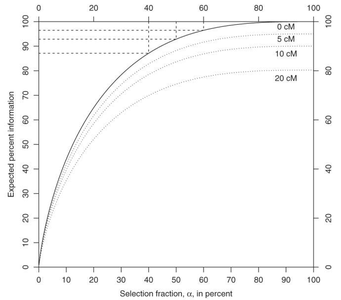
Expected information from a selectively genotyped backcross as a function of the selection fraction (α, the proportion of extreme phenotypic individuals genotyped) in the middle of a marker interval of length 0 cM, 5 cM, 10 cM, and 20 cM. The information is plotted relative to fully genotyped cross where all individuals are genotyped at a dense set of markers. We can see that if the cross is densely genotyped, genotyping between 40% and 60% of the cross gives us between 85% and 95% of the information in the cross. The gains diminish with wider marker spacings. The figure was created using the function info.

For a further discussion of information content in the context of genetic-mapping experiments see Sen et al. (2005).

Implementation

Using the theory described above, we have developed a computer package written in the open source R programming language (Ihaka and Gentleman 1996). The package may be downloaded from http://www.biostat.ucsf.edu/sen/software.html. For those unfamiliar with R, the website has instructions on how to get started using the package.

Functions

The main user functions in the package are:

• powercalc calculates power to detect a QTL given effect size, residual error variance, genome-wide threshold, width of marker interval containing QTL, sample size, and proportion of extreme individuals genotyped (selection fraction).

• detectable calculates minimum detectable QTL effect as a function of target power and other powercalc inputs.

• samplesize calculates minimum sample size needed to detect QTL effect given power and other powercalc inputs.

• info calculates approximate expected information as a function of the selection fraction and marker interval width.

• optspacing calculates optimal marker spacing and selection fraction given genotyping cost and the genome size.

• optselection calculates optimal selection fraction given genotyping cost, marker spacing, and genome size.

• error.var calculates residual error variance given cross type, environmental variance, background genetic variance, and number of environmental replicates per unique genotype.

• thresh calculates the genome-wide LOD threshold required for QTL detection given the cross type, genome length, and marker density using the approximations of Dupuis and Siegmund (1999).

All user functions are documented. For example, to access documentation for the function powercalc, the user would type “help(powercalc).”

Assumptions

We assume that the phenotype distribution is Gaussian, the effect size is small relative to the residual variance, and that the sample size is large (a warning is printed if the effective sample size is smaller than 30). The Gaussian assumption facilitates analytical tractability; and the sample size assumption is needed to use the χ² approximations for power calculations. The small effect size assumption simplifies information content calculations; the resulting approximation is accurate for most practical situations. We also assume that the measurement error is negligible. If that is not the case, it may be advisable to consider replicating measurements.

Cost functions are assumed to be linear; this ignores economies of scale but is a useful guide. The optimal marker spacing and selection fractions therefore should be seen as approximations and not strictly optimal. The function approximating the residual error variance assumes that all loci are additive. This is intended as an approximation; in practice one would consider a range of possibilities (see examples below). We also assume that measurement error is negligible. If that is not the case, measurements should be replicated. Finally, we note that we focus on design options for detecting a QTL. For localizing a QTL, other criteria apply (Darvasi 1998).

Examples

Traditional QTL power calculations use proportion of the variance attributable to a locus. These can be calculated using the function detectable (Table 3). The proportion of variance attributable to a QTL has to be interpreted in the context of the cross, the mode of action of the locus (Table 1), the error variance which depends on the number of environmental replicates per genotype, and the cross type (Table 2). Little power is lost by spacing markers 5–10 cM apart relative to dense genotyping and by genotyping half of the most extreme phenotypic individuals. However, we note that it is desirable to genotype at least half of the cross for robustness. A cursory glance at Table 3 may give the impression that there is little difference between a backcross and an intercross. However, as discussed in the Theory section, the allelic effects that can be detected in an intercross are smaller. We illustrate this with an example using the package. We calculate the minimum effect size detectable with 80% power with 100 individuals typing markers densely.

Table 3.

The minimum percentage variance attributable to a QTL for it to be detectable with 80% power as a function of sample size, marker spacing (in cM), and selection fraction (proportion of extreme phenotypic individuals genotyped)

	Selection fraction
	100%				50%
Sample size	Marker spacing in cM				Marker spacing in cM
n	0	5	10	20	0	5	10	20
Backcross
100	17.9	18.7	19.5	21.4	19.1	19.9	20.7	22.7
200	9.9	10.3	10.8	12.0	10.5	11.0	11.6	12.8
400	5.2	5.4	5.7	6.4	5.6	5.8	6.1	6.8
F2 intercross
100	20.8	21.7	22.6	24.7	22.1	23.0	23.9	26.1
200	11.6	12.2	12.7	14.1	12.4	13.0	13.6	15.0
400	6.2	6.5	6.8	7.6	6.6	6.9	7.3	8.1

The LOD threshold to declare significance is calculated using the method of Dupuis and Siegmund (1999). We use the threshold of 3.2 for backcross and 4.2 for F₂ intercross. This is the calculated threshold corresponding to dense markers for the mouse genome (1450 cM). The power is calculated for a locus at the center of a marker interval with the given spacing.

We first calculate the appropriate LOD threshold to use for the mouse genome of size 1440 cM using the thresh function.

> thresh(G=1440,cross=“bc”, p=0.05)[1] 3.189658

In the computer output examples, lines with the “>“ character denote user inputs. Above, we told the thresh function that we wanted the 5% threshold (p=0.05) for a genome of length 1440 cM (G=1440) in a backcross population (cross=“bc”). We get the analogous threshold for the F₂ intercross as follows:

> thresh(G=1440,cross=“f2”, p=0.05)[1] 4.182964

Then we calculate the minimum detectable effect sizes using the function detectable.

> dectable(cross=“bc”, n=100, sigma2=1) thresh=3.2)effect percent.var.explained[1,]0.9360905     17.97001>detectable(cross=“f2”, n=100, sigma2=1 thresh=4:2) additive. effect dominance.effect, percent. var. zexplained[1,] 0.7259998 0 20.85714

Although the locus explains a similar percentage of variance in both the backcross and F₂ intercross populations, the effect size that can be detected in the intercross is smaller (assuming no dominance). This is reiterated in the examples below.

The following narrative illustrates how our tools may be used. We emphasize raw variances attributable to a locus so that we can compare competing crossing designs.

(1) Jane is planning to map blood pressure QTLs in mice in an F₂ intercross. The A and B strains have blood pressure means of 85 mm Hg and 105 mm Hg, respectively. The within-strain standard deviations are 8 mm Hg. (We suppress measurement units for brevity below.) An oversight board asks Jane to justify the number of progeny. She wants to know how many mice are needed to detect a QTL with 80% power. She assumes that the QTL is additive, and an allelic substitution raises the blood pressure by 5. We estimate ${\sigma }_E^2$, the environmental variance by the within-strain variance, to be 8² = 64. It is difficult to estimate the background genetic variance without assumptions. We consider a range of possibilities guiding our choices using the between-strain variance, (105 − 85)²/4 = 100. This would be the genetic variance in RI lines if a single QTL accounted for the strain difference. If there are two or more QTL, the genetic variance would be smaller in the absence of epistasis. Thus, consider three values of ${\sigma }_G^2$, 25, 50, and 100 (these correspond to percent variance attributable to the QTL equal to 14.0%, 12.3%, and 9.9%, respectively). For ${\sigma }_G^2=25$, we use:

> samplesize(cross=“f2”, effect=c(5,0),env.var=64,gen.var=25)sample.size percent.var. explained[1,] 121 14.04494

This gives us a sample size of 121. The additive and dominance effects we wish to detect are given in the effect argument. The residual error variance is approximated using our estimates of the environmental and genetic variances (alternatively one can specify the residual error variance directly). If the genetic variance is 50 or 100, we get sample size estimates of 140 and 180, respectively. By default, the software assumes that our target LOD threshold is 3, desired power is 80%, and all individuals are typed densely; these defaults can be overridden.

(2) Her postdoc, John, asks, “Why don't we perform a backcross?” Plugging the three values of ${\sigma }_G^2$, 25, 50, and 100, into samplesize gives us sample sizes of 234, 255, and 296, respectively. Thus, a backcross would involve using more mice than the intercross.

(3) A week later John reports that 30 RI lines bred from the same strains are available. Should the lab use the RI lines? RI lines are most advantageous when the genetic variance is small relative to the environmental variance. Therefore, the best scenario for RI lines would be when ${\sigma }_G^2=25$. Using six mice per RI line would imply a total of 180 mice. To find out how much power we have to detect an additive effect of 5 with 30 RI lines (each replicated 6 times, indicated by the argument bio.rep) we use

> powercalc(cross=ri,n=30,effect=5,env.var=64,gen.var=25,bio.rep=6)  power percent.var.explained[1,] 0.8074976     41.20879

However, if the genetic variance is 50, then even an indefinite number of mice per line would not give sufficient power. Thus, the use of RI lines in this scenario would require additional preliminary data to estimate genetic variance in the RI lines.

(4) Jane finds out that she can afford about 240 mice. What kinds of effects can she reasonably detect? We consider three possibilities: 240 intercross mice, 240 backcross mice, and 8 replicates of 30 RI lines that are available. We assume that we want to detect only additive effects and that the genetic variance is 25. Using the function detectable for the RI lines as follows:

> detectable(cross=“ri”,n=30,env.var = 64, gen.var = 25,bio.rep=8)   effect percent.var. explained[1,] 4.781040 40.92199

we find that an effect of 4.78 or larger can be detected with 80% or more power. Using analogous commands for the backcross and intercross, we find that we can detect additive effects of 4.93 or larger in the backcross and 3.54 or larger in the intercross. Thus, the backcross and RI lines are equally good, but the intercross is better. If the genetic variance exceeds 25, the RI lines are less advantageous.

(5) Jane decides to perform an intercross. How dense should the genotyping be? Should she genotype everyone or a fraction of the mice with extreme blood pressure? The core genotyping facility charges approximately 30 cents a genotype, and the animal facility per diem rate for mice is $1.20. The total cost of housing a mouse for 25 weeks is about $30; therefore, the genotyping cost in the units of raising the mouse is about 0.01. Because the mouse genome size is about 1440 cM (denoted by G), we conclude that it would be best to genotype 25% of each extreme of the animals at approximately 20 cM (the argument sel.frac, denoting the selection fraction, is set to NULL to indicate that we wish to find the optimal selection fraction simultaneously with the optimal spacing):

> optspacing(cost=30/3000,G=1440,sel.frac=NULL,cross=“f2”)Marker spacing (cM), Selection fraction20.92194      0.49043

Discussion

When planning an experiment we have to make design choices to best use available resources using credible information about the unknown state of nature. Our R/qtlDesign software provides tools to plan QTL experiments using crosses between two inbred lines. Our tools help the experimenter choose between cross types, marker density, and selective genotyping strategies using approximate knowledge about the parental strains and the cost structure of the proposed experiment.

In addition to the design choices mentioned above, it is helpful to follow the basic principles of good experimental design. In the context of QTL experiments, this would include adjusting for covariates potentially influencing the phenotype, performing reciprocal crosses (if maternal effects are suspected or if the QTL is X-linked), deciding whether to consider one sex or both, adjusting for litter or foster mom effects, etc.

Because our software is open source, our algorithms and implementation are transparent to the interested user. Users may modify the code to fit their needs after agreeing to the GNU General Public License (http://www.gnu.org/copyleft/gpl.html). We will continue to make improvements to the software by incorporating new developments and user needs. We hope that our software will be a useful resource for the complex trait community.

References

- 1.Belknap JK. Effect of within-strain sample size on QTL detection and mapping using recombinant inbred mouse strains. Behav Genet. 1998;28:29–38. doi: 10.1023/a:1021404714631. [DOI] [PubMed] [Google Scholar]
- 2.Broman KW. Review of statistical methods for QTL mapping in experimental crosses. Lab Anim. 2001;307:44–52. [PubMed] [Google Scholar]
- 3.Broman KW, Wu H, Sen S, Churchill GA. R/qtl: QTL mapping in experimental crosses. Bioinformatics. 2003;19:889–890. doi: 10.1093/bioinformatics/btg112. [DOI] [PubMed] [Google Scholar]
- 4.Cox D, Hinkley D. Theoretical Statistics. Chapman and Hall; London: 1974. [Google Scholar]
- 5.Darvasi A. Experimental strategies for the genetic dissection of complex traits in animal models. Nat Genet. 1998;18:19–24. doi: 10.1038/ng0198-19. [DOI] [PubMed] [Google Scholar]
- 6.Dupuis J, Siegmund D. Statistical methods for mapping quantitative trait loci from a dense set of markers. Genetics. 1999;151:373–386. doi: 10.1093/genetics/151.1.373. [DOI] [PMC free article] [PubMed] [Google Scholar]
- 7.Flint J, Valdar W, Shifman S, Mott R. Strategies for mapping and cloning quantitative trait genes in rodents. Nat Rev Genet. 2005;6:271–286. doi: 10.1038/nrg1576. [DOI] [PubMed] [Google Scholar]
- 8.Ihaka R, Gentleman R. R: A language for data analysis and graphics. J Comput Graph Stat. 1996;5:299–314. [Google Scholar]
- 9.Kearsey M, Pooni HS. The Genetical Analysis of Quantitative Traits. Chapman and Hall; London: 1996. [Google Scholar]
- 10.Lynch M, Walsh B. Genetics and analysis of quantitative traits. Sinauer Associates Inc; Sunderland, MA: 1998. [Google Scholar]
- 11.Purcell S, Cherny SS, Sham PC. Genetic Power Calculator: design of linkage and association genetic mapping studies of complex traits. Bioinformatics. 2003;19:149–150. doi: 10.1093/bioinformatics/19.1.149. [DOI] [PubMed] [Google Scholar]
- 12.Rapp JP. Genetic analysis of inherited hyper-tension in the rat. Physiol Rev. 2000;80:131–172. doi: 10.1152/physrev.2000.80.1.135. [DOI] [PubMed] [Google Scholar]
- 13.Sen S, Satagopan JM, Churchill GA. Quantitative trait loci study design from an information perspective. Genetics. 2005;170:447–464. doi: 10.1534/genetics.104.038612. [DOI] [PMC free article] [PubMed] [Google Scholar]
- 14.Silver LM. Mouse genetics. Oxford University Press; Oxford: 1995. [Google Scholar]