Sparseness prior based iterative image reconstruction for retrospectively gated cardiac micro-CT

Abstract

Recent advances in murine cardiac studies with three-dimensional (3D) cone beam micro-CT used a retrospective gating technique. However, this sampling technique results in a limited number of projections with an irregular angular distribution due to the temporal resolution requirements and radiation dose restrictions. Both angular irregularity and undersampling complicate the reconstruction process, since they cause significant streaking artifacts. This work provides an iterative reconstruction solution to address this particular challenge. A sparseness prior regularized weighted l₂ norm optimization is proposed to mitigate streaking artifacts based on the fact that most medical images are compressible. Total variation is implemented in this work as the regularizer for its simplicity. Comparison studies are conducted on a 3D cardiac mouse phantom generated with experimental data. After optimization, the method is applied to in vivo cardiac micro-CT data.

I. INTRODUCTION

Imaging cardiac structure and function in mice is challenging due to the small size of their heart (long axis is about 7 mm) and their rapid heart rate (up to 600 beats per minute). Thus, both high spatial and temporal resolutions are necessary for functional murine cardiac imaging. In vivo cardiac imaging is currently performed with MR microscopy,^1–4 echocardio-graphic techniques,³ or with micro-CT.^5,6

Previously, we characterized cardiac structure and function in mice using a prototype micro-CT system providing four-dimensional (4D) data sets with an isotropic spatial resolution of 100 μm and a temporal resolution of 10 ms.⁵ This work used prospective cardiorespiratory gating. This gating approach ensures uniform and sufficient angular sampling but involves long acquisition time since the images are triggered by the coincidence of two events, i.e., the end expiration in the breathing cycle and the imaging time point (e.g., systole, diastole) in the cardiac cycle. Recently, Drangova et al.⁶ have described retrospective gating for cardiac micro-CT that provided a fast imaging option with a spatial resolution of 150 μm and a temporal resolution of 12 ms. In retrospective gating, the projections are sampled with an equiangular step but at various points in the cardiac and breathing cycle. Both ECG and a respiration signal are recorded and used in postprocessing to cluster the projections in sets corresponding to the cardiac and respiratory phases to be reconstructed. For each of the cardiac phases, the corresponding projections have an irregular angular distribution, since many views may be missing. The number of projections for each phase may be further limited when many cardiac phases are to be reconstructed from a limited number of projections. Because of this irregular and undersampled pattern, the reconstructed images are affected by noise and streaking artifacts, when analytical reconstruction algorithms such as Feldkamp's⁷ are used.⁶

This article presents a reconstruction algorithm designed to address these problems in the reconstruction stage, so that retrospective gating with reduced number of projections can be adopted to yield both reduced sampling time and reduced radiation dose. More specifically, we describe an algorithm for cone beam CT reconstruction based on sparseness prior and a filter-weighted least-square cost function. In particular, minimum total variation (TV) is implemented as the sparseness prior. TV has been described in the literature as a method for noise reduction and debluring (also known as restoration) in two-dimensional (2D) medical images.^8–11 Compared to the widely used quadratic functions,¹² the TV norm is very good at preserving edges, without introducing ringing or blurring artifacts. The TV regularizer has been used previously in 2D PET imaging,¹³ diffraction tomography,¹⁴ and computed tomography.^15,16 The technique was extended to three-dimensional (3D) for limited view angle ectomography.¹⁷ Very recently, in the series works of “compressed sensing” and “robust uncertainty principles,” TV, as well as some other sparse transformations, have been demonstrated in optimal and near-optimal signal reconstruction from incomplete linear measurements.^18–22 These theories are being quickly adapted and applied on spiral and radial MR image reconstructions.^23–25 Least-square (or in many cases, weighted least-square) cost functions have also been found in the literature for sinogram data noise reduction on low-dose x-ray CT reconstruction by penalizing the weighted least-square with a quadratic term.^26–28 In those studies, the least square term was weighted by the variances of the repeated projection measurements at each bin. In comparison, this work uses a filtering matrix to weight the least-square term, for the purpose of faster convergence. To our knowledge, this is the first time the filter-weighted least-square approach penalized by TV has been used for cone beam CT data, especially addressing the undersampling and irregularity in retrospective gating.

II. MATERIALS AND METHODS

II.A. Imaging system

The imaging system used in this work has been described in detail in Ref. 29. The system uses a high-flux rotating anode x-ray tube (Philips SRO 09 50) designed for clinical angiography, with a dual 0.3/1.0 mm focal spot operating at 9kW (0.3 mm focal spot) or 50 kW (1.0 mm focal spot). The detector is a cooled, charge-coupled device camera with a Gd₂O₂S phosphor on a 3:1 fiber optic reducer (X-Ray Image Star, Photonics Science, East Sussex, UK). The camera has an active input area of 106 mm (horizontal) ×106 mm (vertical) imaged on the sensor with an image matrix of 2048×2048 pixels with pixel size of 51×51 μm. The tube and detector are mounted in the horizontal plane on an extruded aluminum frame (80/20, Bellevue, WA). The animal is held in a vertical position in an acrylic cradle using an upper incisor bar and the limbs are taped to the side of the cradle. The cradle is then placed on a circular pedestal that is rotated about the vertical axis by a computer-controlled stepping motor (Oriel Model 13049). The distance between the detector and animal is 40 mm and the distance between the animal and x-ray source is 480 mm. This configuration results in a geometric blur of the focal spot that matches the Nyquist sample at the detector²⁹ with limiting spatial resolution of 100 μm in the object. The x-ray parameters used in this study are as follows: 80 kVp, 170 mA, and 9 ms exposure per projection.

Cardiac micro-CT studies require both the use of contrast agents and an integrated motion control, i.e., gating strategies to deal with respiratory and cardiac motion. In our work, we use injections of a blood contrast agent Fenestra™ VC (ART Advanced Research Technologies, Saint-Laurent, Quebec, Canada) with doses ranging from 0.013 to 0.02 ml/g animal during our studies. This results in enhancement higher than 300 HU between the blood and left ventricle allowing successful segmentation of the blood pool.

The respiratory gating strategy was always prospective, i.e., we used intubation and ventilation of the animals and imaging triggered only during end expiration of the breathing cycle. In previous work, we described a prospective approach regarding cardiac motion. In that work, the acquisition of each projection was triggered when the predefined phase of the cardiac cycle occurred in the predefined window during end expiration.⁵

In this study, we have implemented retrospective cardiac gating in which projections are always acquired during end expiration, but in randomly occurring phases of the cardiac cycle. Retrospective gating requires recording of the ECG signal, the angular information and the sampling time points during acquisition. The sampling, monitoring, and data store are achieved using a custom LabVIEW application (National Instruments, Austin, TX). The recorded physiologic signals and angular position are used in the postprocessing to tag projections with their angle and the cardiac phase. This clustering of data is implemented in MATLAB (The MathWorks, Natick, MA). The process starts by the detection of the R peaks in the ECG signal. Next, each projection is registered with the ECG signal by detecting the closest two R peaks to the projection sampling time. Each R−R interval in the ECG cycle is divided in the number of temporal intervals equal to the cardiac phases to be reconstructed. Each projection is assigned to the corresponding cardiac phase according to the time interval where the sampling occurred.

The number of projections acquired during a micro-CT study varies with the sampling time, radiation dose, and image quality requirements, but is always less than 400 for a single (phase) 3D data set. When cine-cardiac imaging is required, the number of projections can reach thousands, depending on the temporal resolution, i.e., the number of phases in the cardiac cycle.

For routine studies, the 2D planar projection images are used to reconstruct 3D image arrays using a modified Feldkamp algorithm.^5,7 The software reconstructs the data onto a 100 μm isotropic grid which is essentially the limit imposed by the geometry and Nyquist sample at the detector.

II.B. Filtered backprojection with irregular and insufficient angular sampling

We performed phantom simulations to demonstrate the problems associated with retrospective gating. Specifically, we explored the influence of the number of projections and the effect of irregular angular sampling on image quality, when a conventional reconstruction method such as filtered backprojection is used. We used the 3D mouse cardiac phantom developed by Paul Segars et al.³⁰ for these simulations. The phantom was modeled with nonuniform rational b-spline surface based on data collected at the Duke Center for In Vivo Microscopy. The original phantom was modified to reflect the use of contrast agent in our cardiac experiment, i.e., the voxels corresponding to the blood in the heart were set to a value to be about 1.3 times of those corresponding to the soft tissue. This corresponds to a difference of 300 HU between the myocardium and the blood in the left ventricle that is obtainable using Fenestra VC.⁵

A single 2D slice (256×256) from the 3D mouse phantom is used in these simulations. We used a random selection of fan beam projections over the entire 180° sampling arc to simulate irregular angular sampling. The reconstruction is performed using filtered backprojection in matlab. The reconstructed image from projections sampled at the Nyquist sampling rate was compared to those from undersampled projection data. Approximately 400 regular projections are needed to meet the Nyquist limit imposed by angular sampling. For comparison, undersampling with only 100 and 50 regular projections were also simulated.

II.C. TV-CT reconstruction

The TV algorithm is implemented as the sparseness transform. A previous work on limited view angle ectomography¹⁷ extended the 2D definition to 3D. In analogy to Ref. 17, the 3D TV term of an image f in this work is defined as follows:

$${\Vert \phi \left(f\right)\Vert }_{l_1}=\int \mid \nabla f\mid dxdydz=\int \sqrt{\nabla f_x^2+\nabla f_y^2+\nabla f_z^2}dxdydz,$$ (1)

where φ takes the finite difference of the three-dimensional image and ∥ · ∥_ll takes the l₁ norm of the transform coefficients. In a discrete version, Eq. (1) becomes

$${\Vert \phi \left(f\right)\Vert }_{l_1}=\sum _{i,j,k}\sqrt{{(\nabla f_x^2)}_{i,j,k}+{(\nabla f_y^2)}_{i,j,k}+{(\nabla f_z^2)}_{i,j,k}+\eta },$$ (2)

where ▽f_x, ▽f_y, and ▽f_z represent the finite differences of the image along x, y, and z direction and the spatial discretization steps have been assumed unity. η is a small positive number to avoid singularities in Eq. (2).

With the TV term defined above, we describe the TV regularized CT iterative reconstruction method. We consider the ideal projection signal model as s=Pf, where s is the projection data vector, P represents the system or projection matrix, and f is the vector of attenuation coefficients, i.e., the image to be reconstructed. Our TV-CT iterative reconstruction algorithm solves the image via the following optimization problem:

$$\underset{\forall f}{\min }{\Vert \phi \left(f\right)\Vert }_{l_1}s.t.Pf=s.$$ (3)

In reality, the projection measurements do contain noise and other imperfections so it is more practical to use an inequality linear constraint as in Eq. (4),

$$\underset{\forall f}{\min }{\Vert \phi \left(f\right)\Vert }_{l_1}s.t.{\Vert Pf=s\Vert }_2^2\le \epsilon ,$$ (4)

where ε is a small positive number that is set based on level of measurement noise. The constrained optimization in Eq. (4) can either be solved directly by linear programming methods such as projection onto convex set³¹ or be converted to an unconstrained optimization

$$\tilde{f}=\underset{\forall f}{\arg \min g}\left(f\right)=\underset{\forall f}{\arg \min \mu }\frac{{\Vert \phi \left(f\right)\Vert }_{l_1}}{{\Vert f\Vert }_{l_1}}+\frac{{\Vert Pf-s\Vert }_D^2}{{\Vert s\Vert }_2^2}$$ ( 5 )

and then solved with iterative solvers. Note that in Eq. (5), instead of the l₂ norm used in the constraint of Eq. (4),a D weighting matrix is added in the least-square term. μ is the normalized regularization parameter and it is dimensionless and unitless. As a result, the cost function g(f) in Eq. (5) consists of components from both image-space regularization, i.e., the l₁ norm term and projection data fidelity, i.e., the least-square term. The regularization parameter adjusts the relative penalties on the sparseness and the data fidelity. μ can be tuned to favor high edge and resolution performances or fidelity to the measurements based on the specific interest of an application. The D weighting is purposely included as a preconditioner to accelerate the convergence. In theory, the algorithm can almost converge in one iteration, if P^HDP=I, where P^H denotes the Hermitian of P and I is the identity matrix. Solving for D could be complicated and time consuming. However, a practical approximation is that the P^HD operator be implemented using filtered backprojection. Possible choices of filters include the CT ramp filter with a Ram-Lak, Hanning, or Hamming window. Such choices of filter improves the condition of the system matrix P and guarantee near optimal convergence.

The nonlinear conjugate gradient (CG) method is used to solve the optimization problem in Eq. (5) iteratively. The nonlinear CG method generalizes the conjugate gradient method to nonlinear optimization and is used to find the local minimum of a nonlinear function using its gradient.^32,33

During each CG iteration, the cost function and its gradient are calculated given the current image. The subgradient of the cost function is

$$\nabla g\left(f\right)=\mu \nabla {\Vert f\Vert }_{\mathrm{TV}}∕{\Vert f\Vert }_1+2P^{H}D(Pf-s)∕{\Vert s\Vert }_2^2,$$ (6)

where the subgradient of the TV term is derived as

$$\nabla {\Vert \phi \left(f\right)\Vert }_{l_1}=h_{i-1,j,k}^x-h_{i,j,k}^x+h_{i,j-1,k}^y-h_{i,j,k}^y+h_{i,j,k-1}^z-h_{i,j,k}^z,$$ (7)

with

$$\begin{array}{cc}\hfill h_{i,j,k}^x& =\frac{{(\nabla f_x)}_{i,j,k}}{\sqrt{{(\nabla f_x^2)}_{i,j,k}+{(\nabla f_y^2)}_{i,j,k}+{(\nabla f_z^2)}_{i,j,k}+\eta }},\hfill \\ \hfill h_{i,j,k}^y& =\frac{{(\nabla f_y)}_{i,j,k}}{\sqrt{{(\nabla f_x^2)}_{i,j,k}+{(\nabla f_y^2)}_{i,j,k}+{(\nabla f_z^2)}_{i,j,k}+\eta }},\hfill \\ \hfill h_{i,j,k}^z& =\frac{{(\nabla f_z)}_{i,j,k}}{\sqrt{{(\nabla f_x^2)}_{i,j,k}+{(\nabla f_y^2)}_{i,j,k}+{(\nabla f_z^2)}_{i,j,k}+\eta }}.\hfill \end{array}$$ (8)

Our tests for TV-CT reconstruction included the influence of the projection number on image quality and the comparison of the TV-CT method with the Feldkamp algorithm. The mean square errors (MSE) and maximum errors (ME) were plotted against the number of projections and used as figures of merit that allowed an objective comparison of the algorithms.

The MSE between the reconstructed image f̃ and the true phantom image f is defined as MSE(f̃)=∥f̃−f∥_l2/∥f∥_l2, where ∥x∥_l2=x'x and x is a column vector. The ME was defined as $\mathrm{ME}\left(\tilde{f}\right)=\max (\tilde{f}-f)∕\sqrt{({\Vert f\Vert }_{l2}∕N)}$, where N is the total number of pixels in the image.

To study the convergence of the TV-CT iterative method, we stopped the iterations with a threshold on the number of iterations although in practical applications a threshold on the cost function will be more reasonable and easy to implement. For all cases, 20 iterations were used and the cost function was monitored at each iteration.

II.D. Animal experiments

All animal studies were conducted under a protocol approved by the Duke University Institutional Animal Care and Use Committee. Two 25 g C57BL/6 mice were used in this study. The animals were anesthetized with Ketamine (115 mg/kg, 20 mg/ml, 0.17 ml) and Diazepan (27 mg/kg, 0.5 mg/ml, 0.16 ml) and peroraly intubated for mechanical ventilation using a ventilator described previously³⁴ at a rate of 120 breaths/min with a tidal volume of 0.4 ml. A solid-state pressure transducer on the breathing valve measured airway pressure and electrodes (Blue Sensor, Medicotest, UK) taped to the animal footpads acquired ECG signal. Both signals were processed with Coulbourn modules (Coulbourn Instruments, Allentown, PA) and displayed on a computer monitor using a custom-written LabVIEW application. Body temperature was recorded using a rectal thermistor and maintained at 36.5°C by an infrared lamp and feedback controller system (Digi-Sense®, Cole Parmer, Chicago, IL). A catheter was inserted following a tail vein cut down and used for the injection of a blood pool contrast agent Fenestra™ VC (ART Inc., Quebec, Canada) with a dose of 0.5 ml/25 g mouse as recommended by the manufacturer. Animals were placed in a cradle and scanned in a vertical position. During imaging, the anesthesia was maintained with 1%−2% isoflurane.

In order to study the effect of irregular and angular undersampling with real data, we first performed an experiment with prospective gating and Nyquist sampling. We collected 380 projection images over 190° with prospective gating on the R peak in the ECG signal. Total acquisition time was 4 min. We simulated retrospective gating by randomly selecting 95 projections, i.e., 1/4 of the total number of projections acquired. We kept the prospective case data, i.e., uniformly sampled case with 380 projections and reconstructed using filtered backprojection algorithm as a reference for image quality to which we compared the reconstructions with nonuniformly distributed and limited number of projections corresponding to retrospective gating. The simulated retrospective projection data was used both with filtered backprojection and TV-CT reconstruction algorithms.

In a second experiment with a different mouse, we performed imaging using a truly retrospective gating approach. 1800 projection images were acquired during a single rotation over an angle of 190°. The total acquisition time was 15 min. The projections were next clustered in ten phases of the cardiac cycle. For the two phases, i.e., diastole and systole, the projection data sets contained 182 and 161 projections, respectively. The two cardiac phases were reconstructed using both filtered backprojection and TV-CT (five iterations).

III. RESULTS

The results of the simulations are shown in the first row of Fig. 1. Use of only 100 views [Fig. 1(b)] results in subtle background artifacts, but they are not readily visible in the central part of the image. Artifacts with regular sampling become problematic when the number of views is reduced to 50 [Fig. 1(c)]. The second row of Fig. 1 shows the results of these simulations when the same number of views is distributed randomly. Even with Nyquist sampling, i.e., 400 projections, the artifacts associated with irregular projection angles are apparent. As the angular sampling is decreased, the streaking artifacts become much more apparent.

Fig. 1.

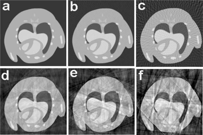
The influence of the number of projections and the angular distribution in image quality when filtered backprojection in fan beam reconstruction is used: (a) uniform angles 400 projections, (b) uniform angles 100 projections, (c) uniform angles 50 projections, (d) random angles 400 projections, (e) random angles 100 projections, and (f) random angles 50 projections.

Figure 2 shows simulations comparing results of undersampling when using the modified Feldkamp algorithm⁷ used in our system and the TV-CT reconstruction in 3D. For the image size 128×128×128, Nyquist sampling requires 210 projections. In this study, we used 210, 140, 70, and 35 projections, corresponding to 1, 2/3, 1/3, and 1/6 of Nyquist sampling rate. For each case, we compared the TV-CT iterative reconstruction (top row) with filtered backprojection via the Feldkamp algorithm⁷ (bottom row). The results are shown in axial view, which is of most interest for cardiac study. Note that even with Nyquist sampling, irregular angles cause visible artifacts in the filtered backprojection reconstructed image. By comparison, the TV-CT method provides reconstruction of high fidelity. The simulated phantom images shown in Figs. 1 and 2 were windowed in the range [0, 0.0025]. Undersampling further aggravates the artifacts in the filtered backprojection reconstructions. The resolution is significantly diminished and many details of interest are lost. The results produced by TV-CT have consistently fewer streaking artifacts. In particular, with 35 projections, the image reconstructed with the TV-CT algorithm retains all the important information in and around the heart, while filtered backprojection suffers from the severe streaking artifacts.

Fig. 2.

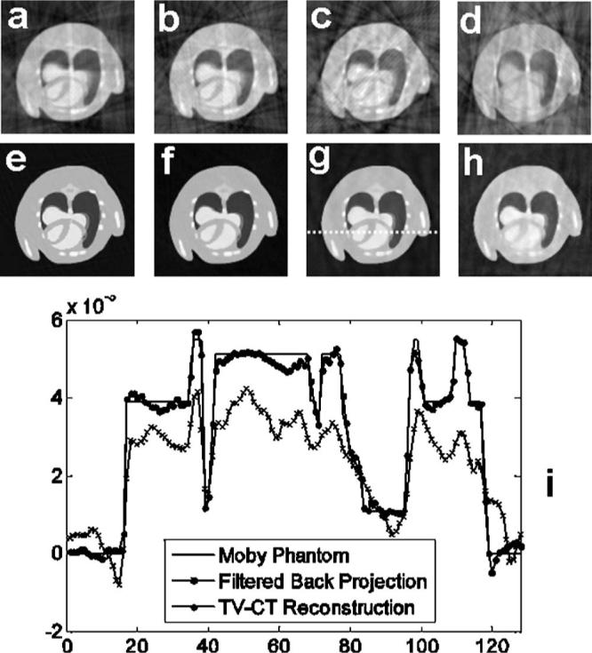
Comparison of filtered backprojection and TV-CT reconstruction with irregular and undersampled projections. Filtered backprojection using (a) 210, (b) 140, (c) 70, and (d) 35 random projections. TV-CT reconstruction using (e) 210, (f) 140, (g) 70, and (h) 35 random projections. (i) A line profile comparison extracted from the 70-projection case.

Figure 3 plots the cost values against the number of iterations to indicate the speed of convergence and the final cost level when converged. The plots are generated in a log-linear style. Figure 3(a) shows that the curves for all cases converge within ten iterations. In Fig. 3(b), the convergence curve for the 70-projection case reconstructed with weighting is compared to the one without weighting. The advantage of using the weighting, i.e., the filter D in Eq. (3), is visible in the convergence curve.

Fig. 3.

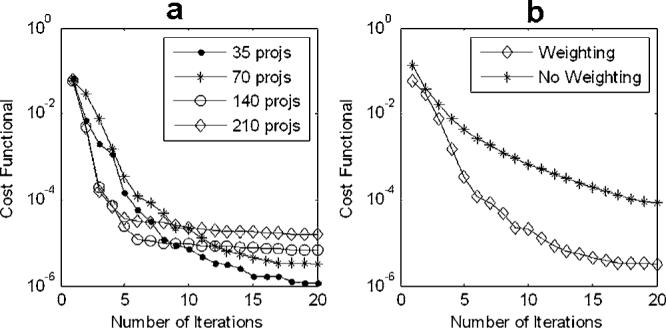
Convergence curves (cost values plotted against number of iterations) for TV-CT reconstruction methods applied on irregular and undersampled projections. (a) Comparison of convergence curves for the 210, 140, 70, and 35-projection case. (b) Comparison of convergence curves for the 70-projection case with and without weighting on the l2 norm term.

MSE and the ME of the reconstructed images are also plotted against the number of projections in Figs. 4(a) and 4(b), for both filtered backprojection and TV-CT iterative reconstruction. We computed MSE and ME in a relative sense and show it as a percentage. The shape of the curves suggests the effectiveness of the corresponding reconstruction method on irregular and undersampled projection measurements. The closer the curves are to the origin of the coordinate, the more efficient the method is. Figure 4 indicates that MSEs and MEs of TV-CT reconstructions in all cases are significantly lower than those of filtered backprojection. One sees a general trend for both curves where the MSE and ME are smaller when more projections are used. However, an exception is observed for the 140-projection case with TV-CT method. An explanation of this is that the random projections are generated independently among these cases. Some cases have a more irregular pattern than the others. It was noted in the simulations in Fig. 1 that irregularity impacts the image quality more than the undersampling rate. The 140-projection case may have more severe artifacts than the 105-projection case, and as a result, the case converges to a higher cost level. The same effect is seen for 105 projections using filtered backprojection.

Fig. 4.

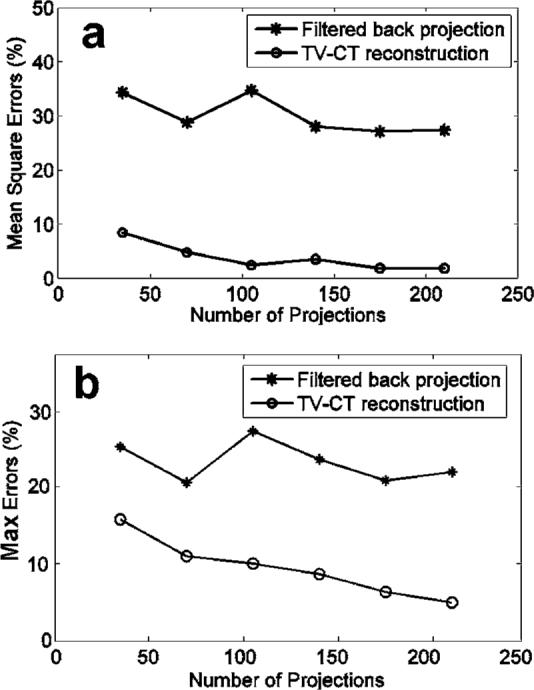
Plots of mean square errors (a) and maximum errors (b) of the reconstructed images against number of projections used in the reconstruction. Curves for filtered backprojection and TV-CT iterative method are included.

Figure 5 presents three orthogonal cuts from a 512×512×128 array reconstructed from the prospectively gated data, as well as randomly undersampled data simulated from this original data set. Note the striking difference in image quality between the filtered backprojection and TV-CT with the simulated retrospective gating. As shown here the image quality using TV-CT becomes adequate even when the number of projections available is reduced to 95.

Fig.5.

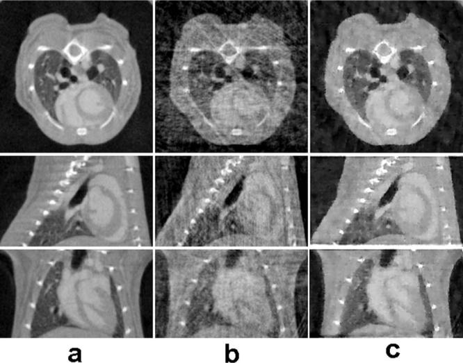
In vivo cardiac micro-CT images reconstructed from prospectively (a) and simulated retrospectively gated 3D cone-beam measurements (b), (c).In (a) filtered backprojection reconstruction was used with 380 prospectively gated projections, while (b) and (c) show results for using 95 retrospectively gated projections with filtered backprojection reconstruction and TV-CT reconstruction, respectively.

Figure 6 presents the both axial and coronal slices from a 512×512×128 array reconstructed from data acquired with truly retrospective gating. Both Feldkamp's algorithms and TV-CT reconstruction were performed for two time points in the cardiac cycle corresponding to diastole and systole. Figures 5 and 6 were windowed in the range [−1000, 1000] HU for an objective comparison. The improvement in image quality in the TV-CT reconstructions is quite clear.

Fig. 6.

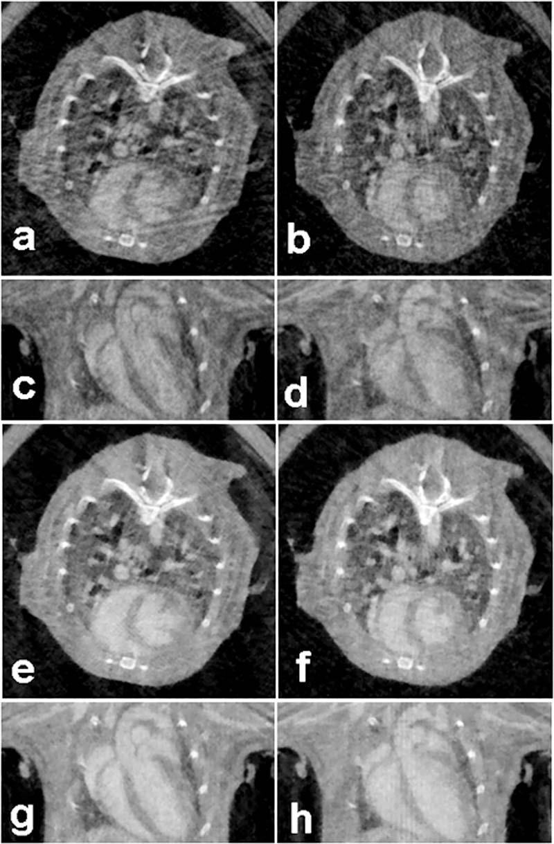
Axial and coronal micro-CT slices obtained using retrospective gating corresponding to diastole [(a), (c), (e), (g)] and systole [(b), (d), (f), (h)] and reconstructed with filtered backprojection [(a), (b), (c), (d)] and TV-CT [(e), (f), (g), (h)].

The reconstruction was conducted on a Apple Mac computer with a Dual 1.42 GHz power PC G4 processor and a 2GB DDR SDRAM memory. A processing time measure indicated that our implementation of the forward projection and backprojection of the volume took about 25 min. During the acquisition of the prospective data set on a single point in the cardiac cycle, the radiation dose was 0.21 Gy. For the retrospective gating experiment with 1800 projections acquired, the measured dose was 1.04 Gy.

IV. DISCUSSIONS

The assumption of compressibility is critical to the use of sparseness prior in our algorithm. While most of the medical images are indeed compressible, the choice of “best basis” varies, as well as how sparse the coefficients could be with that choice. This work found total variation was actually a very effective, robust, and simple one and it worked well on our simulations cases as well as real measurements. Some “blocky” effects were observed but they were very minor compared to the improvements [see Fig. 5(c)].

In our TV-CT algorithm, there are a few parameters that need to be set before the execution. These include regularization factor μ and iteration stopping threshold.

The regularization factor is selected to leverage the cost function's emphasis on the sparseness prior and the weighted l₂ norm distance. The determination of this regularization factor has been always an interesting area of research in the field of regularized iterative methods.^35–37 A well-known method to find such factor is via the L curve, but this approach is very costly. In our studies, we empirically determined the regularization factor, for example, μ=1.5×10⁻¹⁰ is used for the phantom study. Since the optimization was normalized and μ is now unitless, it should be generally around this number for similar images. A useful rule of thumb is that this factor should be selected large when the image is sparser. Intuitively, this can be interpreted as that the reconstruction relies more on the sparseness prior.

The iteration stopping threshold defines when the convergence is considered to be reached. It caps the relative changes in the optimization cost. This threshold therefore has direct impact on the number of iterations needed for convergence as well as the image quality. Setting the threshold low will result in more accurate reconstruction (lower MSE) but longer reconstruction time. In our studies, a threshold of 0.001 and proved to be a reasonable choice.

The reason of including the weighting on the l₂ norm term is to speed up the convergence. The weighting improves the condition of the projection matrix. However, in our implementation, we never attempted to find the precondition matrix D, but instead implemented it using a CT filter in the Fourier domain. The conventional filters used in filtered backprojection methods effectively get P^HDP very close to an identity matrix therefore the speed up of convergence is significant, if not optimal. However, it should be noticed that this weighting also increases the emphasis of cost function on high frequency signals, since these filters amplify high frequencies more than the low frequencies. In other words, the optimization goal is slightly changed, though no visible differences were observed on the image quality in our studies. We experimented with several different filters and found the Hanning and Hamming filters performed slightly better than the Ram-Lak filter.

As shown by our results (see Figs. 5 and 6), the image quality with TV-CT using retrospective gating is high and amenable to automated image analysis required to quantify the volume of the left ventricle and provide functional cardiac measures such as ejection fraction, cardiac output and stroke volume.⁵ Figure 5 suggests that very limited number of projections, i.e., only 95 acquired using retrospective gating would provide sufficient image quality. This suggests that we can reduce the number of projections to less than 1000 for a complete 4D data set with ten phases during cardiac cycle and voxel size of 100 μm. The associated radiation dose can therefore be reduced to 0.55 Gy. This makes our sampling more dose efficient. Drangova et al.⁶ have described a retrospective method with a lower dose but larger voxels (150 μm versus 100 μm in this work). Our approach of prospective gating for the respiration combined with retrospective gating on the ECG signal has the advantage that all projection data is used unlike in Ref. 6, where the projections acquired during inspiration are discarded.

The major limitations of the present approach is the longer time associated with the iterative reconstruction methods. In the TV-CT method, forward projection of the image (applying the P operator) and the filtered backprojection (i.e., P^HD operator) of the residual projection data have to be computed repeatedly. The total reconstruction time is therefore directly proportional to the time calculating projection and backprojection. It becomes very helpful if this time can be reduced. Several strategies for reducing the time for reconstruction have potential. Work by Benson et al.³⁸ suggests significant improvement using a method terms “focus of attention.” New computational engines based on accelerated graphic chips or new cell processors promise computational improvements of 10−100×.³⁹

V. CONCLUSIONS

Our previous work with 4D micro-CT of the mouse heart has generated exciting new possibilities for functional phenotyping. But two barriers limit the application: acquisition time and dose. We have shown here a sparseness prior based iterative reconstruction method for retrospectively gated cardiac micro-CT data that addresses both of these barriers. Acquisition of retrospectively gated date with reduced number of views is very straightforward. Unfortunately the irregular projection angles as well as undersampling from retrospective gating cause significant artifacts in the images reconstructed with traditional cone beam algorithms. The proposed method solves a total variation regularized weighted l₂ norm optimization with conjugate gradient solver. The performance of the method has been validated on both phantom and real mouse heart data. Significant improvements on SNR, resolution, and artifact reduction have been demonstrated using this method compared to conventional filtered backprojection method. The convergence of the method is fast, due in part to the weighting in the optimization function. The method improves the dose efficiency and the sampling time while providing image quality required for studies of anatomical and functional phenotyping in rodents.

References

- 1.Ruff J, Wiesmann F, Hiller KH, Voll S, Von Kienlin M, Bauer WR, Rommel E, Neubauer S, Haase A. Magnetic resonance microimaging for noninvasive quantification of myocardial function and mass in the mouse. Magn. Reson. Med. 1998;40:43–48. doi: 10.1002/mrm.1910400106. [DOI] [PubMed] [Google Scholar]
- 2.Cassidy PJ, Schneider JE, Grieve SM, Lygate C, Neubauer S, Clarke K. Assessment of motion gating strategies for mouse magnetic resonance at high magnetic fields. J. Magn. Reson. Imaging. 2004;19:229–237. doi: 10.1002/jmri.10454. [DOI] [PubMed] [Google Scholar]
- 3.Dawson D, Lygate CA, Saunders J, Schneider JE, Ye X, Hulbert K, Noble JA, Neubauer S. Quantitative 3-dimensional echocardiography for accurate and rapid cardiac phenotype characterization in mice. Circulation. 2004;110:1632–1637. doi: 10.1161/01.CIR.0000142049.14227.AD. [DOI] [PubMed] [Google Scholar]
- 4.Schneider JE, Cassidy PJ, Lygate C, Tyler DJ, Wiesmann F, Grieve SM, Hulbert K, Clarke K, Neubauer S. Fast, high-resolution in vivo cine magnetic resonance imaging in normal and failing mouse hearts on a vertical 11.7 T system. J. Magn. Reson. Imaging. 2003;18:691–701. doi: 10.1002/jmri.10411. [DOI] [PubMed] [Google Scholar]
- 5.Badea CT, Fubara B, Hedlund LW, Johnson GA. 4D micro-CT of the mouse heart. Mol. Imaging. 2005;4:110–116. doi: 10.1162/15353500200504187. [DOI] [PubMed] [Google Scholar]
- 6.Drangova M, Ford NL, Detombe SA, Wheatley AR, Holdsworth DW. Fast retrospectively gated quantitative four-dimensional (4D) cardiac micro computed tomography imaging of free-breathing mice. Invest. Radiol. 2007;42:85–94. doi: 10.1097/01.rli.0000251572.56139.a3. [DOI] [PubMed] [Google Scholar]
- 7.Feldkamp LA, Davis LC, Kress JW. Practical cone-beam algorithm. J. Opt. Soc. Am. 1984;1:612–619. [Google Scholar]
- 8.Rudin LI, Osher S, Fatemi E. Nonlinear total variation based noise removal algorithms. Physica D. 1992;60:259–268. [Google Scholar]
- 9.Chan TF, Mulet P. Iterative methods for total variation image restoration. J. Num. Anal. 1999;36 SIAM (Soc. Ind. Appl. Math.) [Google Scholar]
- 10.Vogel CR, Oman ME. Fast, robust total variation-based reconstruction of noisy, blurred images. IEEE Trans. Image Process. 1998;7:813–824. doi: 10.1109/83.679423. [DOI] [PubMed] [Google Scholar]
- 11.Chan T, Marquina A, Mulet P. High-order total variation-based image restoration. SIAM J. Sci. Comput. (USA) 2000;22:503–516. [Google Scholar]
- 12.Tikhonov AN. On the stability of inverse problems. Dokl. Akad. Nauk SSSR. 1943;39:195–198. [Google Scholar]
- 13.Jonsson E, Huang S-C, Chan T. Total variation regularization in positron emission tomography. U.C.L.A. Comput. Appl. Math. Rep. 1998;98–48 [Google Scholar]
- 14.Bronstein MM, Bronstein AM, Zibulevsky M, Azhari H. Reconstruction in diffraction ultrasound tomography using nonuniform FFT. IEEE Trans. Med. Imaging. 2002;21:1395–1401. doi: 10.1109/TMI.2002.806423. [DOI] [PubMed] [Google Scholar]
- 15.Zhang X-Q, Froment J. Total variation based Fourier reconstruction and regularization for computer tomography; IEEE Nuclear Science Symposium; 2005.pp. 2332–2336. [Google Scholar]
- 16.Delaney AH, Bresler Y. Efficient edge-preserving regularization for limited-angle tomography; Proceedings of the International Conference on Image Processing; 1995.pp. 176–179. [Google Scholar]
- 17.Persson M, Bone D, Elmqvist H. Total variation norm for three-dimensional iterative reconstruction in limited view angle tomography. Phys. Med. Biol. 2001;46:853–866. doi: 10.1088/0031-9155/46/3/318. [DOI] [PubMed] [Google Scholar]
- 18.Candès EJ, Romberg J, Tao T. Robust uncertainty principles: Exact signal reconstruction from highly incomplete frequency information. IEEE Trans. Inf. Theory. 2006;52:489–509. [Google Scholar]
- 19.Candès EJ, Romberg J. “Practical signal recovery from random projections,” Wavelet Applications in Signal and Image Processing XI. Proc. SPIE. 2005;5674:76–86. [Google Scholar]
- 20.Candès EJ, Romberg J, Tao T. Stable signal recovery from incomplete and inaccurate measurements. Commun. Pure Appl. Math. 2006;59:1207–1223. [Google Scholar]
- 21.Candès E, Romberg J. Quantitative robust uncertainty principles and optimally sparse decompositions. Found. Comput. Math. 2006;6:227–254. [Google Scholar]
- 22.Donoho D. Compressed sensing. IEEE Trans. Inf. Theory. 2006;52:1289–1306. [Google Scholar]
- 23.Lustig M, Donoho DL, Pauly JM. Rapid MR imaging with compressed sensing and randomly under-sampled 3DFT trajectories; Proc. 14th Annual Meeting of ISMRM; 2006. [Google Scholar]
- 24.Chang T-C, He L, Fang T. MR image reconstruction from sparse samples using Bregman iteration; Proc. 14th Annual Meeting of ISMRM; 2006. [Google Scholar]
- 25.Plett ILJ, Guarini M, Irarrazaval P. Comparison of wavelets and a new DCT algorithm for sparsely sampled reconstruction; Proc. 14th Annual Meeting of ISMRM Annual Conference; 2006. [Google Scholar]
- 26.Li T, Li X, Wang J, Wen J, Lu H, Hsieh J, Liang Z. Nonlinear sinogram smoothing for low-dose x-ray CT. IEEE Trans. Nucl. Sci. 2004;51:2505–2513. [Google Scholar]
- 27.La Rivière PJ, Billmire DM. Reduction of noise-induced streak artifacts in x-ray computed tomography through spline-based penalized-likelihood sinogram smoothing. IEEE Trans. Med. Imaging. 2005;24:105–111. doi: 10.1109/tmi.2004.838324. [DOI] [PubMed] [Google Scholar]
- 28.Wang J, Li T, Lu H, Liang Z. Penalized weighted least-squares approach for low-dose x-ray computed tomography. SPIE Med. Imaging. 2006;6142:1369–1380. doi: 10.1109/42.896783. [DOI] [PMC free article] [PubMed] [Google Scholar]
- 29.Badea C, Hedlund LW, Johnson GA. Micro-CT with respiratory and cardiac gating. Med. Phys. 2004;31:3324–3329. doi: 10.1118/1.1812604. [DOI] [PMC free article] [PubMed] [Google Scholar]
- 30.Segars WP, Tsui BMW, Frey EC, Johnson GA, Berr SS. Development of a 4-D digital mouse phantom for molecular imaging research. Mol. Imaging Biol. 2004;6:149–159. doi: 10.1016/j.mibio.2004.03.002. [DOI] [PubMed] [Google Scholar]
- 31.Bregman LM. Finding the common point of convex sets by the method of successive projection. Dokl. Akad. Nauk. USSR. 1965;162:487–490. [Google Scholar]
- 32.Fletcher R, Reeves CM. Function minimization by conjugate gradients. Comput. J. 1964;7:149–154. [Google Scholar]
- 33.Briggs WL. A Multigrid Tutorial. SIAM; Philadelphia, PA: 1987. [Google Scholar]
- 34.Hedlund LW, Johnson GA. Mechanical ventilation for imaging the small animal lung. ILAR J. 2002;43:159–174. doi: 10.1093/ilar.43.3.159. [DOI] [PubMed] [Google Scholar]
- 35.Thompson AM, Brown JC, Kay JW, Titterington DM. A study of methods of choosing the smoothing parameter in image restoration by regularization. IEEE Trans. Pattern Anal. Mach. Intell. 1991;13:326–339. [Google Scholar]
- 36.O'Leary DP. Near-optimal parameters for tikhonov and other regularization methods. SIAM J. Sci. Comput. 2001;23:1161–1171. [Google Scholar]
- 37.Kilmer ME, O'Leary DP. Choosing regularization parameters in iterative methods for ill-posed problems. SIAM J. Matrix Anal. Appl. 2001;22:1204–1221. [Google Scholar]
- 38.Benson TM, Gregor J. Phys. Med. Biol. 2006;51:4533–4546. doi: 10.1088/0031-9155/51/18/006. [DOI] [PubMed] [Google Scholar]
- 39.Kachelriess M, Knaup M, Bockenbach O. Hyperfast parallel-beam and cone-beam backprojection using the cell general purpose hardware. Med. Phys. 2007;34:1474–1486. doi: 10.1118/1.2710328. [DOI] [PubMed] [Google Scholar]