

Abstract
Molecular dynamics (MD) simulations of the activation domain of porcine procarboxypeptidase B (ADBp) were performed to examine the effect of using the particle-particle particle-mesh (P3M) or the reaction field (RF) method for calculating electrostatic interactions in simulations of highly charged proteins. Several structural, thermodynamic, and dynamic observables were derived from the MD trajectories, including estimated entropies and solvation free energies and essential dynamics (ED). The P3M method leads to slightly higher atomic positional fluctuations and deviations from the crystallographic structure, along with somewhat lower values of the total energy and solvation free energy. However, the ED analysis of the system leads to nearly identical results for both simulations. Because of the strong similarity between the results, both methods appear well suited for the simulation of highly charged globular proteins in explicit solvent. However, the lower computational demand of the RF method in the present implementation represents a clear advantage over the P3M method.
Keywords: Molecular dynamics, electrostatics, procarboxypeptidase B, solvation, entropy, essential dynamics
The proper treatment of electrostatic interactions is one of the most crucial points for the calculation of accurate forces in molecular dynamics (MD) simulations of biomolecules. In addition, the computation of the electrostatic forces is generally the most computationally demanding task in those simulations. In systems containing a large number of atoms, for example, large protein in explicit solvent, this computational cost can be reduced by the use of rapid but approximate methods. Two components in which accuracy has commonly been traded for speed are electronic polarizability and long-range interactions (Gilson 1995). The methods used for the treatment of electrostatic interactions typically split the force on each charge into a short- and a long-range contribution, and use approximations for dealing with the latter. The simplest approximation is to neglect the long-range contribution. However, electrostatic interactions are truly long-ranged, and straight truncation (i.e., the use of a cutoff applied to Coulomb interactions) may significantly alter the simulated properties of the system (Schreiber and Steinhauer 1992; Hünenberger and van Gunsteren 1998).
A first better approximation is the application of a generalized reaction field (RF) term based on the Poisson-Boltzmann approach (Tironi et al. 1995). In the RF method, each charge is individually considered as the origin of a spherical coordinate system. It is surrounded by a cutoff sphere containing explicit neighboring particles, itself placed within a homogeneous dielectric continuum of permittivity equal to that of the solvent and of specified ionic strength. The equations of continuum electrostatics are solved using spherical symmetry to estimate the reaction-field force from the continuum onto the particle. This long-range correction is added to the short-range contribution computed by explicit summation over the neighboring atoms within the cutoff sphere. The result is a simple modification of the pairwise Coulomb forces that entails only a slight increase in computational costs. Although the applicability of this method to nonhomogeneous systems (e.g., protein in water) can be questioned, because the cutoff spheres of the different particles are surrounded by portions of the system which may not respond as a homogeneous dielectric medium, it has been shown to improve dramatically the simulation results compared to straight truncation of the Coulomb interactions (Gargallo et al. 2000). In homogeneous systems such as pure liquid water where this ambiguity does not exist, the inclusion of an RF correction also results in a dramatic improvement of results compared to straight truncation (Hünenberger and van Gunsteren 1998).
The second common approximation to handle the long-range component electrostatic interactions is to assume their exact periodicity within the simulated system, as is done in lattice-sum methods. Under this approximation, electrostatic interaction can be computed in an accurate and computationally efficient way by using the particle-particle particle-mesh (P3M) method (Hockney and Eastwood 1998; Luty and van Gunsteren 1996). Like the RF method, the P3M approach relies on a splitting of the total interaction between particles into a short-range component, which is computed by direct particle-particle summation, and a long-range component, which is computed (under the approximation of a perfectly periodic system) using Fourier series. In contrast to the Ewald method (Allen and Tildesley 1987), which evaluates the Fourier series directly, the P3M method takes advantage of computationally efficient fast Fourier transform algorithms. The short-range contribution to the nonbonded interactions (which include dispersion, repulsion, and the short-range component of electrostatics interactions) is calculated by explicit particle-particle summation with (minimum-image) spherical truncation.
Although lattice-sum methods are often believed to provide “exact” electrostatic interactions, the applicability of these methods to inherently nonperiodic systems (e.g., solutions) may also be questioned, because of the artificial periodicity they imposed on the simulated system. Previous investigations of solvated biomolecules have suggested that artificial periodicity may significantly perturb conformational equilibrium, resulting in smaller fluctuations and an artificial stabilization of the most compact state (Hünenberger and McCammon 1999a; Weber et al. 2000). The magnitude of periodicity-induced artifacts is larger in solvents of low dielectric permittivity, for solute cavities of nonnegligible size compared to the unit cell size, and for solutes bearing a large overall charge (Hünenberger and McCammon 1999b).
The main goal of the present study was the comparison of the RF and P3M methods for the calculation of electrostatic interactions in MD simulations of a highly charged protein. Several thermodynamic and structural parameters, together with the computer times required to complete the calculations, were used as a measure of the accuracy and efficiency of both methods for calculations in large molecular systems.
The activation domain of porcine procarboxypeptidase B (ADBp), which corresponds to the N-terminal globular 75-residue part of the prosegment, is used as a model system. It consists of a four-stranded antiparallel β-sheet with two α-helices and one 310-helix packed over its external face, in an antiparallel α/antiparallel β topology (Coll et al. 1991). The structure has two internal salt bridges (4Glu-49Arg, 49Arg-30Asp) and is free of disulfide bridges. ADBp was chosen for several reasons. First, despite a relatively small size, it shows a high degree of secondary structure. Second, it bears a relatively large net charge (Gargallo et al. 2000), which makes it particularly well suited for a comparison of methods to compute electrostatic interactions. Third, the activation domain interacts with the enzyme by a docking mechanism, and the study of essential dynamics (ED; Amadei et al. 1993) in this region (around helix 310) is of special interest. Finally, the protein system associated with the activation domain of procarboxypeptidase was used previously as a model system for detailed studies of protein folding and unfolding (Villegas et al. 1995, 1998; Fernandez et al. 2000).
Results
Computational expenses
The computer (CPU) time required to perform the simulation is an important issue. For the protein system considered in the present study and on our computer (see Computation Procedure), a 100 psec MD simulation using the RF method for the calculation of electrostatics interactions requires about 5 CPU h. In contrast, a 100 psec MD simulation using the P3M method under the conditions employed here (see Computation Procedure) requires about 90 CPU h for completion.
Structural parameters
The root mean square deviation (RMSD) is a simple measure of the difference between the protein structures sampled along the simulation and the crystallographic structure (Coll et al. 1991). The time evolution of the RMSD (backbone atoms) is displayed in Figure 1a ▶ for the simulations employing the RF and P3M methods. Both simulations reached a structural equilibrium after about 1200 psec. The RF simulation was extended to 5 nsec, and the profile was consistent with a structural equilibrium reached after about 1200 psec. However, overall the RF simulation is characterized by a smaller deviation from the crystallographic structure, with an RMSD value of 1.5–2 Å over the second half of the trajectory. The P3M simulation is characterized by a slightly higher RMSD value of 2–2.5 Å over the second half of the trajectory. On the other hand, the dynamics of the ions showed a large mobility in both simulations. The mean square positional fluctuation for the sodium ions was around 1175 Å2 for the RF simulation and 707Å2 for the P3M simulation, and for chloride ions these values were around 2777Å2 and 1437Å2 for the RF and P3M simulations, respectively. These results indicate a somewhat larger mobility of the ions along the RF simulation compared to P3M. This difference may arise from the approximation nature of the long-range forces in the RF simulation or from the presence of larger force fluctuations in this simulation (cutoff noise). Nevertheless, this effect can only be appreciated on free species such as ions, but did not affect the protein.
Figure 1.

Time evolution of conformational features and solvation energies. Time evolution of the root-mean-square atomic positional deviation (RMSD) from the crystallographic structure for backbone atoms (a), radius of gyration for backbone atoms (b), solvation free energy (c), and polar and nonpolar surfaces (d). Thin line, RF simulation; thick line, P3M simulation. Conformations were sampled every 25 psec.
The time evolution of the radius of gyration (backbone atoms), which gives information on the evolution of the overall shape of the protein, is shown in Figure 1b ▶. A radius of gyration larger than that of the crystallographic structure (11.0 Å) indicates an expansion of the protein. For both simulations, the protein reached a structural equilibrium at similar values of the radius of gyration, very close to the experimental value for the native state (~11.0 Å).
The hydrogen bonds present in the crystallographic structure were analyzed along the simulations. On average, 43% and 44% of the native crystallographic hydrogen bonds are preserved during RF and P3M simulations, respectively. However, the distribution of the conserved hydrogen bonds is different for backbone and side chains. Whereas backbone hydrogen bonds are well preserved (59.5% for RF and 60.3% for P3M), side-chain hydrogen bonds are almost systematically lost (8.3% for RF and 4.2% for P3M). From the hydrogen bond analysis, there is therefore hardly any difference between RF and P3M simulations.
Solvation free energy and solvent-accessible surface area
The solvation free energy evaluated for 100 configurations sampled every 25 psec during the two simulations is displayed as a function of the corresponding RMSD value in Figure 1c ▶. On average, this quantity is more negative for the P3M simulation (−3310 kcal/mole) compared to the RF simulation (−3250 kcal/mole).
The polar and nonpolar solvent-accessible surface areas (SASAs) computed for the crystallographic structure are reported in Table 1, together with the corresponding mean values for RF and P3M simulations. The corresponding time evolution of the surface area components is displayed in Figure 1d ▶. Compared to the crystallographic structure, the total SASA is increased by 1.7% in the RF simulation and 5.1% in the P3M simulation. In the RF simulation, the ratio of polar and nonpolar exposed surface area is essentially the same as in the native structure. In contrast, for the P3M simulation, the increase in the SASA is almost exclusively due to an increase in the polar exposed surface. This observation may explain in part the more favorable solvation free energies characterizing the solute configurations issued from the P3M simulation.
Table 1.
Solvent-accesible surface area (SASA)
| Parameter | X-ray | RF | P3M | |
| Total surface | [A2] | 4865.2 | 4947.4 | 5113.2 |
| Polar surface | [A2] | 2996.1 | 3028.7 | 3244.1 |
| [%] | 61.6 | 61.1 | 63.4 | |
| Nonpolar surface | [A2] | 1869.2 | 1918.7 | 1869.1 |
| [%] | 38.4 | 39.0 | 36.6 |
Polar (O and N atoms), nonpolar (C atoms) and total (polar plus nonpolar) accessible area calculated as the sum of area for the corresponding atoms and its percentage. X-ray, crystallographic structure; RF and P3M, averaged values during the RF or P3M simulations (interval 500–2000 psec).
Figure 2 ▶ shows the total (polar and nonpolar) SASA per residue averaged along each of the two simulations. Hydrophobic regions (Lys5–Val9, Ser18–Glu22 and Val46–Arg49) tend to show the smallest exposed surfaces. With only a few exceptions, the RF and P3M simulations lead to similar values for the average exposed surface per residue. However, the segment including α-helix 1, β-strand 2, as well as the loop between α-helix 2 and β-strand 4 is less exposed in the RF simulation compared to the P3M simulation. In the opposite, the 310 helix and α-helix 2 are more exposed in the RF simulation. These differences remain limited (less than 10% of the residue surface).
Figure 2.

Solvent accessible surface area (SASA) per residue. Total (polar and nonpolar) percentage of SASA per residue, averaged over the RF and P3M (interval 500–2000 psec) simulations. Thin line, RF simulation; thick line, P3M simulation. Values are given in relation to the extended side chain.
Energetic properties
The mean and standard deviations of the total potential and electrostatic energies are reported in Table 2, along with the box volume. The P3M method leads to a lower value of the potential energy. This lower value is an immediate consequence of a lower electrostatic energy. The van der Waals and covalent energy terms do not show a strong dependence on the method employed for the calculation of electrostatic interactions. On the other hand, the time evolution of the potential energy calculated for the RF simulation shows smaller fluctuations compared to the P3M simulation. The volume of the computational box is systematically smaller in the P3M simulation.
Table 2.
Evolution of energies and volume
| Energetic quantity | Method | Mean | Standard deviation |
| Potential energy (kJ/mole) | RF | −189.58 | 1.50 |
| P3M | −196.32 | 1.71 | |
| Electrostatic energy (kJ/mole) | RF | −218.54 | 1.44 |
| P3M | −225.26 | 1.66 | |
| Volume (A3) | RF | 138.06 | 0.35 |
| P3M | 136.52 | 0.34 |
Mean and standard deviation values for the total potential energy, electrostatic energy, and volume for the RF and P3M simulations.
Estimated upper-bound values of the entropy term (TΔS) for backbone atoms are 1521 kcal/mole for the 500–2000 psec segment of the RF simulation and 1590 kcal/mole for the 500–2000 psec segment of the P3M simulation. The higher value for the entropy calculated from the P3M simulation reflects the larger fluctuations in atomic positions (Table 3).
Table 3.
Essential dynamics
| RF | P3M | |||||
| Eigenvector | Eigenvalue [%] | Cumulated eigenvalues [%] | Cumulated TΔS [kcal/mole] | Eigenvalue [%] | Cumulated eigenvalues [%] | Cumulated TΔS [kcal/mole] |
| 1 | 15.29 | 15.29 | 4.57 | 13.09 | 13.09 | 4.52 |
| 2 | 15.18 | 30.47 | 9.14 | 12.98 | 26.07 | 9.03 |
| 3 | 10.49 | 40.96 | 13.59 | 12.01 | 38.08 | 13.53 |
| 4 | 10.47 | 51.42 | 18.05 | 11.80 | 49.88 | 18.01 |
| 5 | 7.97 | 59.39 | 22.42 | 8.29 | 58.17 | 22.40 |
| 6 | 7.93 | 67.32 | 26.80 | 8.15 | 66.32 | 26.77 |
| 7 | 1.22 | 68.55 | 30.61 | 1.64 | 67.96 | 30.67 |
| 8 | 1.21 | 69.76 | 34.41 | 1.63 | 69.59 | 34.57 |
| 9 | 1.09 | 70.85 | 38.20 | 1.28 | 70.87 | 38.39 |
| 165 | 0.08 | 90.02 | 519.16 | 0.08 | 90.14 | 517.93 |
| 903 | 0.00 | 100.00 | 1521.26 | 0.00 | 100.00 | 1590.10 |
Essential dynamics analysis of the two MD simulations (backbone atoms). Eigenvectors are listed in order of decreasing eigenvalues. Eigenvalues are expressed relative to the total mean-square atomic positional fluctuation (trace of the eigenvalue matrix). RF and P3M: values calculated for the RF or P3M simulations (interval 500–2000 psec).
Essential dynamics
The atomic motions along the RF and P3M simulations were analyzed using the essential dynamics (ED) method. The first 500 psec were skipped (equilibration), and the analysis was performed over the intervals 500–1000 psec, 500–1500 psec, and 500–2000 psec for both RF and P3M simulations. The results for the latter interval describe the individual and cumulated contribution of the eigenvectors to the mean-square atomic positional fluctuations and to the entropy, as presented in Table 3. The results for the two other intervals are very similar (data not shown). In all cases, this analysis shows that only 4–5 eigenvectors are required to account for ~50% of the mean-square atomic positional fluctuations. This implies that there are only a few important essential modes of motions, the remaining modes being related to less relevant small-amplitude fluctuations.
To evaluate the consistency of these important essential modes along and among the simulations, the overlap between the major modes (i.e., those accounting for either 50% or 70% of the total mean-square fluctuation, see Table 3) calculated from three different segments of the two simulations is reported in Table 4. When considering the eigenvectors accounting for 50% of the total fluctuations, the subspaces defined by corresponding 4–5 eigenvectors almost completely overlap for the different segments of the two independent simulations. However, when the limit is set to 70% of the total fluctuations, the degree of overlap is slightly lower, which implies that eigenvectors 5 to 9 are either more influenced by random noise or are more specific to a given simulation.
Table 4.
Comparison between essential modes
| RF | P3M | |||||||
| 500–1000 | 500–1500 | 500–2000 | 500–1000 | 500–1500 | 500–2000 | |||
| 50% | RF | 500–1000 | 100 | 91.1 | 88.2 | 98.9 | 90.1 | 86.8 |
| 500–1500 | 100 | 97.1 | 90.6 | 99.2 | 96.2 | |||
| 500–2000 | 100 | 88.4 | 96.9 | 99.5 | ||||
| P3M | 500–1000 | 100 | 91.0 | 87.9 | ||||
| 500–1500 | 100 | 97.0 | ||||||
| 500–2000 | 100 | |||||||
| 70% | RF | 500–1000 | 100 | 96.5 | 88.5 | 89.9 | 89.9 | 87.0 |
| 500–1500 | 100 | 88.4 | 88.8 | 89.7 | 87.1 | |||
| 500–2000 | 100 | 95.9 | 96.1 | 97.2 | ||||
| P3M | 500–1000 | 100 | 98.0 | 97.4 | ||||
| 500–1500 | 100 | 98.8 | ||||||
| 500–2000 | 100 | |||||||
Overlap between the major essential modes calculated for different intervals (psec) of the two MD simulations. The major modes are those accounting for either 50% or 70% of the total mean-square fluctuations (see Table 3). The overlap is expressed in percent.
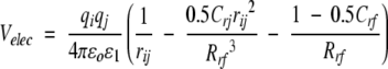
A set of four trajectories involving atomic displacements restricted to be along the first four essential modes (calculated from either the RF or P3M simulations over the interval 500–2000 psec) was generated according to the method of Sherer et al. (1999). The corresponding RMSD values for backbone atoms are displayed in Figure 3A ▶ for each of the four essential modes. Similar graphs were obtained from ED analysis of the other trajectory segments considered in Table 4 (data not shown). The shape of the RMSD profiles is very similar for both simulations, the only difference being that the profiles corresponding to the third and fourth essential modes are interchanged. The RMSD for the first essential mode (Fig. 3A ▶) shows maxima at residues Val11 (β-strand 1), Ala24 (α-helix 1), Ser36 (helix 310), Phe48 (β-strand 3), Phe61 (α-helix 2), and Ile73 (β-strand 4). Several residues do not show any significant motion along this first mode, namely Glu4 (involved in a salt bridge with Arg49), Ile17 (α-helix 1), Asp30 (β-strand 2; also involved in a salt bridge with Arg49), Pro42 (loop between the 310 helix and β-strand 3), Ile55 (beginning of α-helix 2), and Gln68 (beginning of β-strand 4). However, these residues are close to the maxima in the profile corresponding to the second essential mode (Fig. 3A ▶). These maxima are located at residues Arg8 (β-strand 1), Glu19 (α-helix 1), Lys33 (β-strand 2), Val46 (β-strand 3), Ala57 (α-helix 2), and Glu70 (β-strand 4). The residues involved in the third mode for the RF simulation (fourth essential mode for P3M simulation) are those forming the β-strand 2, 310 helix, and β-strand 3. Minima correspond essentially to residues in alpha helices. In contrast, the fourth essential mode for the RF simulation (third essential mode for the P3M simulation) seems to account mainly for the cross-motion of α-helices 1 and 2 (Fig. 3B ▶). Thus, it appears that the dynamic behavior along the RF and P3M simulations is very similar. Moreover, the functional region of the segment, found in strands β2 and β3 and in 310 helix, forming the patch of interaction with the carboxypeptidase, is similarly involved on both simulations, showing correlated maxima and minima. The combined motion of modes 1, 2, 3, and 4 show a correlation between helix 1 and strands 1 and 4, and between helix 2 and strands 2 and 3 (Fig. 3B ▶).
Figure 3.


Analysis of the first four essential modes. (A) RMSD (for backbone atoms) corresponding to a trajectory built along the first four eigenvectors (identified as 1, 2, 3, 4) calculated from the RF and P3M simulations (interval 500–2000 psec). RMSD values were referred to X-ray structure. Thin line, RF simulation; thick line, P3M simulation. (B) Comparison between modes 4 of P3M and 3 of RF and modes 1 and 2 of RF and P3M simulations. Snapshots were taken from the trajectory obtained by the projection of the modes on the simulation. The starting conformation is in green and the last in blue. The X-ray structure of ADBp is shown at the top, indicating the main conformational features; the structure corresponds to the starting structure on the snapshots showing the modes’ motion. Arrows indicate the cross-motion involved with modes 4 of P3M and 3 of RF. The combined motion is shown by arrows taken from modes 1 of P3M and RF (red), modes 2 of P3M and RF (green), and cross-modes 3 and 4 of RF and P3M (in blue and cyan). The motion is represented by a cross that correlates the two portions of the fold: helix 2 with strands 3 and 2; helix 1 with strands 1 and 4.
To further analyze this correlation, the atomic deviations corresponding to the four major essential modes for the RF simulation are plotted against each other in Figure 4 ▶. For the first and second modes, no clear correlation is apparent (Fig. 4A ▶). The corresponding graph for the first and third modes (Fig. 4B ▶) reveals positive or negative correlations for specific segments. For example, a line connecting residues ranging from Ala24 to Ile29 is characterized by a positive correlation. This implies that the motion of this fragment along the first essential mode is almost perfectly correlated with the motion along the third mode. A similar observation can be made for other segments that are either positively (e.g., Lys41 to Asp47) or negatively (e.g., Ser36 to Lys41) correlated along these modes. Correlations among other modes can also be identified (Fig. 4C–F ▶, e.g., segments 25–31, 34–37, 37–40, and 67–74).
Figure 4.
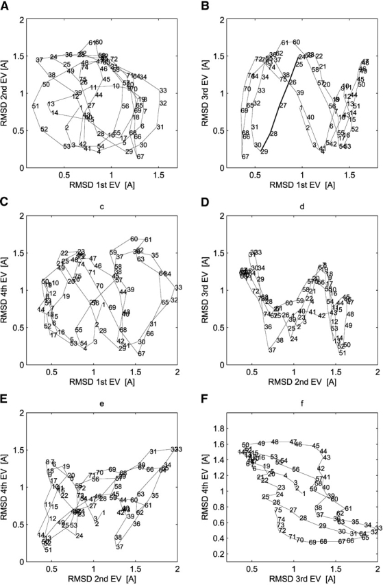
Essential modes correlation. Correlation of RMSD values (backbone atoms) corresponding to a trajectory built along the first four eigenvectors of the RF simulation (interval 500–2000 psec; see Fig. 3 ▶ for the definition of the trajectories).
Discussion
The theoretical backgrounds of RF and P3M approaches are very different. Whereas the P3M method relies on the exact calculation of electrostatic interactions in an infinite periodic system formed by assembling replicas of the reference computational box, the RF method relies on the truncating of coulombic interactions within the periodic system and treating the medium surrounding the cutoff sphere of each atom (or charge group) as a dielectric continuum of permittivity equal to that of the solvent. Following from these two different representations, it is expected that structural and energetic properties obtained from MD simulations using either the P3M or RF method also reflect those differences.
In general, the P3M method appears to evaluate the electrostatic interactions more accurately than the RF method, which is the key argument in favor of this method. In particular, the electrostatic energy calculated with the P3M method is slightly lower than the corresponding value for the RF method (Table 2). Moreover, solvation free energy of the protein calculated from configurations sampled during the P3M simulation is slightly lower compared to the corresponding value for the RF simulation (Fig. 1C ▶), which also hints towards a better description of the protein-solvent interactions. These observations can be explained by a more realistic description of the long-range component of electrostatic interactions obtained with the P3M method. As pointed out earlier, it is not obvious that the RF method is a reasonable approximation when applied to nonhomogeneous systems involving atomic charges located in a heterogeneous dielectric environment (e.g., on protein atoms).
The observed fluctuations in the volume of the computational box are similar for both simulations (Table 2). However, the volume is slightly lower when using the P3M method. This can be understood intuitively, because the P3M approach involves electrostatic interactions for an infinite system and, therefore, formally involves a higher number of atom pairs compared to the RF case. These additional (dominantly attractive) interactions tend to reduce the dimensions of the simulated system. This observation can also be related to the lower values of electrostatic energies calculated with the P3M method. Interestingly, this reduction of the box volume when comparing P3M to RF is not observed for pure solvent simulations (Oliva and Hünenberger 2002). Therefore, it must be associated with differences in the representation of solute-solvent interactions.
The energy profile obtained with the RF method is characterized by smaller fluctuations compared to the P3M simulation (Table 2). This observation is probably related to the lower atomic positional fluctuation RMSD values obtained for the RF simulation. Hence, despite the above discussion, the RF simulation led to a more stable trajectory compared to the P3M method. However, in both cases the native structure of protein is well preserved, and the main features of sampled conformations and surface accessibility are similarly represented by both approaches. The most significant differences between the average structures obtained from the last 1000 psec of both simulations are located in the region of α-helix1, which is the most highly charged secondary structure element present in the protein, including Glu12, Asp13, Glu14, Asp16, Glu19, Glu22, Arg27, and Asp30 (Gargallo et al. 2000).
From the results obtained in this study, it appears that the P3M method offers a slightly better description of the forces acting on a highly charged protein in water compared to the RF method, as evidenced by structural and energetic parameters. This result was already suggested by the analysis of other large charged macromolecular systems such as nucleic acids (Cheatham III et al. 1995; Mafalda and Simonson 2002). However, if the necessity of including long-range electrostatic interactions was previously recognized for these compounds, the case of globular proteins (highly charged ones) had not been systematically investigated. The present study shows the importance of an accurate representation of electrostatic interactions in these systems.
It should be stressed that, in the present implementation, the RF method is computationally less costly than the P3M method. The RF method thus seems to be a more appropriate method for the calculation of electrostatic interactions in large macromolecular systems with the computers available nowadays. On the other hand, tuning the values of some of the parameters could accelerate P3M calculations. In particular, the present P3M calculations used a short-range cutoff of 0.9 nm and a long-range cutoff of 1.2 nm. However, unlike in the RF simulation, only van der Waals interactions are active within the intermediate range 0.9–1.2 nm. Thus, the long-range cutoff could be reduced without significant loss of accuracy, but significantly accelerating the calculations. This was not done in the present study, to permit a comparison between simulations employing the two methods. In addition, the parallelization affects the two methods differently, because, in the present implementation, it applies exclusively to the pairwise (real-space) component of nonbonded interactions, that is, within the short-range cutoff (P3M and RF) and the long-range cutoff (RF only). The parallelization does not apply to the reciprocal space interactions (P3M only) where fast Fourier transforms are performed on a single processor. Therefore, the code for the P3M method could still be improved by further parallelization in the evaluation of reciprocal space interaction.
The dynamic properties of the protein during the two simulations were probed by means of ED (Amadei et al. 1993). The active region of ADBp is located in the segment between β-strand 2 and 310 helix. Therefore, the study of the essential mode dynamics in this region of the protein may provide valuable information related to its biological function (Peters et al. 1997). ED is a powerful tool for finding global, correlated motions in atomistic simulations of macromolecules. Sherer et al. (1999) applied this approach to analyze the covariance matrix obtained along MD trajectories of DNA A-Tract structures. In that work, the ED results showed that only three essential modes were needed to account for almost 60% of the mean-square atomic positional fluctuations. Those principal components were directly related to important functional motions (junction bending, central bending, and helical twisting) of DNA tract structure. In the case of a protein (or a protein fragment such as ADBp), the results of ED are more difficult to rationalize, because of the inherent complexity of proteins compared to nucleic acids. In particular, a large number of eigenvectors are needed to account for the same fraction of the overall mean-square fluctuations. In the present study, it was found that about 10 eigenvectors are needed to account for 70% of the fluctuations and about 160 to reach 90% (Table 3).
The components of the first few eigenvectors corresponding to simulations of large proteins often resemble periodic functions (Hess 2000). Hess derived the form of the principal components based on a model of high-dimensional random diffusion, which is almost periodical. This resemblance between protein motions and random diffusion could imply that, for many proteins, the time scales of current MD simulations are too short to reach convergence of the collective motions. To investigate the differences between the RF and P3M simulation in terms of protein motion, we carried out several ED analyses based on different segments of the two trajectories. The results obtained showed that the (~10) dominant eigenvectors are always very similar (Table 4). The RF simulation was later extended to 5000 psec, and the results of an ED analysis carried out with the 3000–5000-psec interval also agreed very well with those obtained for the 500–2000-psec interval (data not shown). Although the shapes of first and second essential modes (Fig. 3A ▶), which are very similar for the RF and P3M simulations, do resemble cosine curves, we believe that these shapes do not arise from a random diffusion mechanism. As previously mentioned, the first and second essential modes calculated for different intervals of the trajectories are very similar in shape (Fig. 3A ▶) and motion (Fig. 3B ▶), which indicates that the essential modes are actually due to a concerted motion of several segments of the protein (Fig. 3B ▶). This observation and the very close similarity between the RF and P3M results are a clear hint against random-diffusion modes.
A careful study of Figures 3A ▶ and 4 ▶ shows that the residues acting as a hinge between secondary structure elements are Gln28–Asp30 (loop connecting α-helix 1 and β-strand 2), Ile40–Pro42 (loop connecting 310 helix and β-sheet 3), Val50–Ala52 (loop connecting β-sheet 3 and α-helix 2), and Glu66–Gln68 (loop connecting α-helix 2 and β-sheet 4). These residues are found as nodes on the curves describing the fluctuations corresponding to the four main essential modes. Other important residues which could act as central anchors for the structural fluctuations are Val9–Val11 (in the middle of the β-sheet), His21–Ala24 (α-helix 1), Trp32–Pro34 (β-strand 2), Ser36–Thr38 (helix 310), Asp47-Phe48 (β-strand 3), and Asp60–Phe61 (α-helix 2). It should be pointed out that several of these residues are located at the region around β-strand 2 and 310 helix, that is, the region where the activation domain interacts with the rest of the protein. This may reflect the fact that the protein structure was extracted from the crystal structure of the complex, or the natural dynamic instability of a functional region that must accommodate a docking partner.
The transition state in the folding pathway of the human and porcine procarboxypeptidase activation domain I has been investigated by protein engineering approaches (Guasch et al. 1992; Villegas et al. 1998). Like porcine ADBp, activation domain I is a globular domain with no disulfide bridges or cis-Pro bonds, which has been shown to follow a two-state folding transition (Villegas et al. 1995). A protein engineering analysis indicated that the transition state for this activation domain is quite compact, possessing some secondary structure and a hydrophobic core in the process of being consolidated. The core (folding nucleus) was formed by the packing of α-helix 2 and the two central β-strands. The other two strands at the edges of the β-sheet and α-helix 1 appeared to be completely unfolded. The maxima found in the first eigenvector for 310 helix, β-strand 3, and α-helix 2 may thus be related to the folding/unfolding motions that affect the core strands and α-helix 2 (Villegas et al. 1995). Moreover, the correlation of the motion of modes 1, 2, 3, and 4 show that the active patch on the inhibition, formed by strand 2 and the 310 helix, correlates with helix 2 (see Fig. 3B ▶ for the combined motion), where the experimental analyses have already proved the importance of helix 2 in the folding of ADBp.
In conclusion, the present work shows that the RF approach yields results comparable to the P3M approach for a small, highly charged globular protein, at reduced computational costs. This statement is supported by the similarity of the results regarding the conformational space sampled and the dynamic behavior, whereas the energy of the complete system showed the main (yet limited) differences. This conclusion may not be oversimplified to nonhomogeneous macromolecular systems with a very high charge density and anisotropy, as is the case for nucleic acids. However, the present study validates the use of the RF approach for charged proteins, as long as massively parallel computational methods cannot be applied to produce faster simulations with the P3M approach.
Materials and methods
Computation procedure
Molecular dynamics simulations
Two MD simulations were carried out using either the RF or the P3M method for computing electrostatic interactions. In both cases, the GROMOS96 program (van Gunsteren et al. 1996) was used to perform explicit-solvent simulations using the GROMOS 43a1 force field and the SPC/E water model (Berendsen et al. 1987). The crystallographic coordinates of ADBp at 2.3 Å resolution (PDB code 1NSA; Coll et al. 1991) were used as a starting point for the simulations. Eighteen Na+ and seven Cl− ions were added to neutralize the electric charges of ionizable residues. The total number of protein atoms was 789, and the number of water molecules was 4148. The details of the procedure employed to set up the simulations are reported elsewhere (Gargallo et al. 2000). The simulations were carried out for 2000 psec using a time step 0.002 psec. Bond lengths were constrained by application of the SHAKE procedure (Ryckaert et al. 1977). The temperature was maintained at 300 K (solute and solvent separately) and the pressure at 1 atm using a weak-coupling scheme with coupling times of 0.1 psec and 0.5 psec, respectively.
The MD simulations were carried out using a parallelized version of GROMOS96 on an SGI Origin 2000 (CESCA–CEPBA, Barcelona, Spain) with 64 MIPS R10000 processors (each one with a 4-Mb cache) and 8 Gb of main memory.
Electrostatics interactions were calculated by using either the RF or the P3M method. In both cases, the charge group pair list was updated every 10 simulation steps. A cutoff radius (Rc) of 9 Å was chosen to select nearest-neighbor charge groups, and a cutoff radius (Rrf) of 12 Å was used for the long-range electrostatics.
The RF calculations were performed as described (Gargallo et al. 2000). In this scheme, the electrostatic interaction energy between two charges qi and qj (for both solute and solvent sites, and including the generalized Poisson-Boltzmann reaction field contribution) is given by Tironi et al. (1995):
 |
(1) |
where ɛ0 is the dielectric permittivity of the vacuum, ɛ1=1 the relative permittivity of the medium surrounding the simulated particles (vacuum), and Rrf=Rl the (long-range) cutoff distance. The coefficient Crf determines the magnitude of the reaction field forces, and is given by:
 |
(2) |
where ɛ2 is the relative dielectric permittivity of the dielectric continuum, set to ɛ2 = 54 as appropriate for the solvent model used in the simulations.
The P3M calculations were carried out using a modified version of the GROMOS96 program (Scott et al. 1999; Hünenberger 2002) implementing the P3M method for computing electrostatic interactions (Hockney and Eastwood 1988), and an alternative virial expression for calculating the group-based pressure (Hünenberger 2002). The simulation was carried out using a grid size of 64 × 64 × 64 points, a third-order truncated-polynomial charge-shaping function (Hünenberger 2000) of width α = Rc−0.2 nm, a triangular-shaped-cloud assignment scheme (Hockney and Eastwood 1988), and exact differentiation of the gridded potential to obtain the gridded field (Deserno and Holm 1998). The P3M root-mean square force error was reevaluated every 5000 steps, and the influence function was reoptimized when this value exceeded a threshold of 2.0 kJ/mole•nm.
Analysis
Four structural properties of the system were analyzed as function of time: the root-mean-square atomic positional deviation from the crystal structure (RMSD), the radius of gyration (Rg), the hydrogen-bond network within the protein, and the (polar and nonpolar) solvent-accessible surface area (SASA). RMSD values characterize the degree of conformational distortion of the protein compared to its experimentally determined native structure. Changes in the radius of gyration provide an additional measure of global changes in the protein structure. The hydrogen-bond network is used to characterize the stability of the secondary structure. The SASA was calculated atom-wise according to a method described previously (Richmond 1984), and the total surface was accumulated for each residue in order to obtain the percentage of accessibility with respect to an extended side chain.
Several energetic quantities were also analyzed as a function of time: the total potential energy, the electrostatic energy, and estimates of the solvation free energy and entropy of the protein. The solvation free energy was estimated using a finite-difference Poisson-Boltzmann algorithm (Nicholls and Honing 1991) as implemented with the SOLVATE program (Bashford 1997).
The covariance matrix was calculated for the equilibrated portion of each trajectory (interval 500–2000 psec; M configurations) as the 3N × 3N matrix with elements:
 |
(3) |
where xi(k) are the atomic Cartesian coordinates of atom i in configuration k, after applying a least-squares-fit to a common reference structure (X-ray), and ≤xi> is the mean value of the vector coordinates of atom i. The solute entropy was estimated according to the method proposed by Schlitter (1993; Schäfer et al. 2000), as:
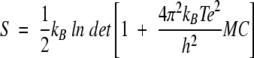 |
(4) |
where kB is Boltzmann’s constant, h Planck’s constant, T the temperature, M is the diagonal 3N × 3N mass matrix, and C the covariance matrix of atomic positional fluctuations. The value of S is an upper-bound estimate corresponding to a harmonic approximation.
ED calculations were also carried out based on the covariance matrix C (Amadei et al. 1993). In this approach, the diagonalization of C to solve the equation:
 |
(5) |
where Λ is a diagonal matrix, provides a set of 3N orthonormal eigenvectors, vn (the columns of the matrix V) with their corresponding eigenvalues λn (the diagonal elements of Λ). The eigenvectors provide a representation of the specific modes of structural deformation of the protein, and the eigenvalue associated with a mode indicates the relative contribution of this mode to the overall protein motion within the simulated trajectory. More precisely, the overall mean-square atomic positional fluctuation is given the trace of Λ whereas the contribution of a specific mode to this number is equal to the corresponding element of Λ. To evaluate the degree of consistency of the essential modes, these were estimated for different portions of the trajectories. The eigenvectors of one trajectory A can be compared with those of another trajectory B by evaluating the overlap γAB between the major eigenvectors vi (i.e., the n eigenvectors with the highest eigenvalues) contained in the corresponding matrices V and V′:
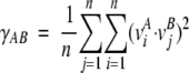 |
(6) |
where n stands for the minimum number of eigenvectors which account for more than a given threshold of the variance of the trajectories (A and B).
Finally, for the ease of interpretation of the deformations associated with each eigenvector, short MD trajectories along the major eigenvectors were generated according to the procedure described by Sherer et al. (1999). These trajectories were generated by changing linearly the coordinate along one essential mode while leaving the coordinates along the others equal to their mean value in the explicit-solvent simulation. The trajectories were analyzed to identify the main contributions of each residue to each essential mode.
Acknowledgments
This work was supported by C4 (CEPBA-CESCA) and by grants from the European Science Foundation, the Spanish Ministerio de Educación y Cultura (CICYT BIO2001-2046 and BIO2002-03609), Fundación Areces, the Swiss National Science Foundation (Project No. 2100-061939), and the CERBA (Centre de Referència en Biotecnologia, Generalitat de Catalunya, Spain). The authors thank J.L. Gelpi, X. de la Cruz, and M. Orozco (University of Barcelona) for providing programs for ED analyses and for useful comments.
The publication costs of this article were defrayed in part by payment of page charges. This article must therefore be hereby marked “advertisement” in accordance with 18 USC section 1734 solely to indicate this fact.
Abbreviations
ADBp, activation domain of porcine procarboxypeptidase B
MD, molecular dynamics
RF, reaction field
P3M, particle-particle particle-mesh
RMSD, root mean square deviation
ED, essential dynamics
Article and publication are at http://www.proteinscience.org/cgi/doi/10.1110/ps.03137003.
References
- Allen, M.P. and Tildesley, D.J. 1987. Advanced simulation techniques. In Computer simulation of liquids. Oxford University Press, New York.
- Amadei, A., Linssen, A.B.M., and Berendsen, H.J.C. 1993. Essential dynamics of proteins. Proteins 17 412–425. [DOI] [PubMed] [Google Scholar]
- Bashford, D. 1997. An object-oriented programming suite for electrostatic effects in biological molecules. In Scientific computing in object-oriented parallel environments. Lecture notes in computer science (eds. Ishikawa et al.), Vol. 1343, pp. 233–240. Springer-Verlag, Berlin.
- Berendsen, H.J.C., Grigera, J.R., and Straatsma, T.P. 1987. The missing term in effective pair potentials. J. Phys. Chem. 91 6269–6271. [Google Scholar]
- Cheatham III, T.E., Miller, J.L., Fox, T., Darden, T.A., and Kollman, P.A. 1995. Molecular dynamics simulations on solvated biomolecular systems: The particle mesh Ewald method leads to stable trajectories of DNA, RNA, and proteins. J. Am. Chem. Soc. 117 4193–4194. [Google Scholar]
- Coll, M., Guasch, A., Avilés, F.X., and Huber, R. 1991. Three-dimensional structure of porcine procarboxypeptidase B: A structural basis for its inactivity. EMBO J. 10 1–9. [DOI] [PMC free article] [PubMed] [Google Scholar]
- Deserno, M. and Holm, C. 1998. How to mesh up Ewald sums. I. A theoretical and numerical comparison of various particle mesh routines. J. Chem. Phys., 109 7678–7693. [Google Scholar]
- Fernandez, A.M., Villegas, V., Martinez, J.C., Van Nuland, N.A.J., Conejero-Lara, F., Avilés, F.X., Serrano, L., Filimonov, V.V., and Mateo, P.L. 2000. Thermodynamic analysis of helix-engineered forms of the activation domain of human procarboxypeptidase A2. Eur. J. Biochem. 267 5891–5899. [DOI] [PubMed] [Google Scholar]
- Gargallo, R., Oliva, B., Querol, E., and Avilés, F.X. 2000. Effect of the reaction field electrostatic term on the molecular dynamics simulation of the activation domain of procarboxypeptidase B. Prot. Eng. 13 21–26. [DOI] [PubMed] [Google Scholar]
- Gilson, M.K. 1995. Theory of electrostatic interactions in macromolecules. Curr. Opin. in Struct. Biol. 5 216–223. [DOI] [PubMed] [Google Scholar]
- Guasch, A., Coll, M., Avilés, F.X., and Huber, R. 1992. Three-dimensional structure of porcine pancreatic procarboxypeptidase A. A comparison of the A and B zymogens and their determinants for inhibition and activation. J. Mol. Biol. 224 141–157. [DOI] [PubMed] [Google Scholar]
- Hess, B. 2000. Similarities between principal components of protein dynamics and random diffusion. Phys. Rev. E 62 8438–8448. [DOI] [PubMed] [Google Scholar]
- Hockney, R.W. and Eastwood, J.W. 1998. Computer simulation using particles. IOP Publishing Ltd., Bristol, England.
- Hünenberger, P.H. 2000. Optimal charge-shaping functions for the particle-particle—particle-mesh (P3M) method for computing electrostatic interactions in molecular simulations. J. Chem. Phys. 113 10464–10476. [Google Scholar]
- ———. 2002. Calculation of the group-based pressure in molecular simulations. I. A general formulation including Ewald and particle-particle-particle-mesh electrostatics. J. Chem. Phys. 116 6880–6897. [Google Scholar]
- Hünenberger, P.H. and McCammon, J.A. 1999a. Effect of artificial periodicity in simulations of biomolecules under Ewald boundary conditions: A continuum electrostatics study. Biophys. Chem. 78 69–88. [DOI] [PubMed] [Google Scholar]
- ———. 1999b. Ewald artifacts in computer simulations of ionic solvation and ion-ion interaction: A continuum electrostatics study. J. Chem. Phys. 110 1856–1872. [Google Scholar]
- Hünenberger, P.H. and van Gunsteren, W.F. 1998. Alternative schemes for the inclusion of a reaction-field correction into molecular dynamics simulations: Influence on the simulated energetic, structural, and dielectric properties of liquid water. J. Chem. Phys. 108 6117–6134. [Google Scholar]
- Luty, B.A. and van Gunsteren, W.F. 1996. Calculating electrostatic interactions using the particle-particle particle-mesh method with nonperiodic long-range interactions. J. Phys. Chem. 100 2581–2587. [Google Scholar]
- Mafalda, N. and Simonson, T. 2002. Molecular dynamics of the tRNAAla acceptor stem: Comparison between continuum reaction field and particle-mesh Ewald electrostatic treatments. J. Phys. Chem. B. 106 3696–3705. [Google Scholar]
- Nicholls, A. and Honing, B. 1991. A rapid finite difference algorithm, utilizing successive over-relaxation to solve the Poisson-Boltzmann equation. J. Comp. Chem. 12 435–440. [Google Scholar]
- Oliva, B. and Hünenberger, P.H. 2002. Calculation of the group-based pressure in molecular simulations. II. Numerical tests and application to liquid water. J. Chem. Phys. 116 6898–6909. [Google Scholar]
- Peters, G.H., van Aalten, D.M.F., Svendsen, A., and Bywater, R. 1997. Essential dynamics of lipase binding sites: The effect of inhibitors of different chain length. Prot. Eng. 10 149–158. [DOI] [PubMed] [Google Scholar]
- Richmond, T.J. 1984. Solvent accessible surface area and excluded volume in proteins. Analytical equations for overlapping spheres and implications for the hydrophobic effect. J. Mol. Biol. 176 63–89. [DOI] [PubMed] [Google Scholar]
- Ryckaert, J.P., Ciccotti, G., and Berendsen, H.J.C. 1977. Numerical integration of the Cartesian equations of motion of a system with constraints: Molecular dynamics of n-alkanes. J. Comp. Chem. 23 327–341. [Google Scholar]
- Scott, W.R.P., Hünenberger, P.H., Tironi, I.G., Mark, A.E., Billeter, S.R., Fennen, J., Torda, A.E., Huber, T., Krüger, T., and van Gunsteren, W.F. 1999. The GROMOS biomolecular simulation program package. J. Phys. Chem. A 103 3596–3607. [Google Scholar]
- Schäfer, H., Mark, A.E., and van Gunsteren, W.F. 2000. Absolute entropies from molecular dynamics simulation trajectories. J. Chem. Phys. 113 7809–7817. [Google Scholar]
- Schlitter, J. 1993. Estimation of absolute and relative entropies of macromolecules using the covariance matrix. Chem. Phys. Lett. 215 617–621. [Google Scholar]
- Schreiber, H. and Steinhauer, O. 1992. Cutoff size does strongly influence molecular dynamics results on solvated polypeptides. Biochem. 31 5856–5860. [DOI] [PubMed] [Google Scholar]
- Sherer, E.C., Harris, S.A., Soliva, R., Orozco, M., and Laughton, C.A. 1999. Molecular dynamics studies of DNA A-tract structure and flexibility. J. Am. Chem. Soc. 121 5981–5991. [Google Scholar]
- Tironi, I.G., Sperb, R., Smith, P.E., and van Gunsteren, W.F. 1995. A generalized reaction field method for molecular dynamics simulations. J. Chem. Phys. 102 5451–5459. [Google Scholar]
- van Gunsteren, W.F., Billeter, S.R., Eising, A.A., Hünenberger, P.H., Krüger, P., Mark, A.E., Scott, W.R.P., and Tironi, I.G. 1996. In Groningen Molecular Simulation (GROMOS) library manual. BIOMOS, Zürich, Switzerland.
- Villegas, V., Azuaga, A., Catasus, Ll., Reverter, D., Mateo, P.L., Avilés, F.X., and Serrano, L. 1995. Evidence for a two-state transition in the folding process of the activation domain of human procarboxypeptidase A2. Biochem. 34 15105–15110. [DOI] [PubMed] [Google Scholar]
- Villegas, V., Martínez, J.C., Avilés, F.X., and Serrano, L. 1998. Structure of the transition state in the folding process of human procarboxypeptidase A2 activation domain. J. Mol. Biol. 283 1027–1036. [DOI] [PubMed] [Google Scholar]
- Weber, W., Hünenberger, P.H., and McCammon, J.A. 2000. Molecular dynamics simulations of a polyalanine octapeptide under Ewald boundary conditions: Influence of artificial periodicity on peptide conformation. J. Phys. Chem. B 104 3668–3675. [Google Scholar]