

Abstract
The goal of this work is to characterize structurally ambivalent fragments in proteins. We have searched the Protein Data Bank and identified all structurally ambivalent peptides (SAPs) of length five or greater that exist in two different backbone conformations. The SAPs were classified in five distinct categories based on their structure. We propose a novel index that provides a quantitative measure of conformational variability of a sequence fragment. It measures the context-dependent width of the distribution of (φ,ξ) dihedral angles associated with each amino acid type. This index was used to analyze the local structural propensity of both SAPs and the sequence fragments contiguous to them. We also analyzed type-specific amino acid composition, solvent accessibility, and overall structural properties of SAPs and their sequence context. We show that each type of SAP has an unusual, type-specific amino acid composition and, as a result, simultaneous intrinsic preferences for two distinct types of backbone conformation. All types of SAPs have lower sequence complexity than average. Fragments that adopt helical conformation in one protein and sheet conformation in another have the lowest sequence complexity and are sampled from a relatively limited repertoire of possible residue combinations. A statistically significant difference between two distinct conformations of the same SAP is observed not only in the overall structural properties of proteins harboring the SAP but also in the properties of its flanking regions and in the pattern of solvent accessibility. These results have implications for protein design and structure prediction.
Keywords: Chameleon sequence, conformational variability, Ramachandran map, intrinsic propensity, local context, secondary structure, entropy
One of the important problems in protein folding is to understand the balance between local and long-range interactions, and their relative contributions to formation of protein structure. The final conformation adopted by a particular residue reflects a combination of environmental factors and intrinsic preference for a specific range of dihedral angles (Griffiths-Jones et al. 1998; Baldwin and Rose 1999). Secondary structure prediction methods rely heavily on intrinsic propensity and local neighbors (Rost and Sander 1994; Garnier et al. 1996). However, local propensity alone does not determine the final conformation of a sequence fragment. For instance, it has been demonstrated, by protein engineering and by analysis of known structures, that certain types of sequence fragments, so-called chameleon sequences, can adopt either α-helical or β-sheet conformations, and a limited number of substitutions can convert a helical protein to a predominantly β-sheet protein (Minor Jr. and Kim 1996; Dalal and Regan 2000). It has also been shown that many short sequence fragments are associated with a broad distribution of local structures rather than with a well-defined structural motif (Rackovsky 1993; Han and Baker 1996). A better understanding of the contribution of intrinsic propensity, sequence context, and other environmental factors to the conformational preference of such structurally ambivalent sequence fragments is important for reliable local structure prediction.
Most scoring functions used in fold recognition use secondary structure propensity encoded in a variety of forms (Bowie et al. 1991; Bahar et al. 1997; Rost et al. 1997; Kuznetsov and Rackovsky 2002). Structurally ambivalent fragments therefore pose a challenge for fold recognition methods. Identification of structurally ambivalent fragments, and determination of the rules governing their conformational preferences, is also important for understanding the mechanism of conformational changes observed in misfolding diseases. One of the best-known examples of misfolding diseases is the group of neurodegenerative disorders (Creutzfeld-Jacob Disease [CJD] scrapie, mad cow disease, etc.) caused by the prion protein, which undergoes a conformational transition from a normal mostly-helical form to a β-sheet–rich pathogenic conformation (Prusiner 1998).
To address the problem of structural variability, one needs to identify conformationally ambivalent segments and to measure the degree of conformational variability of each sequence fragment. A great deal of attention has been paid to systematic identification and classification of sequence patterns with strong conformational preferences (Rooman et al. 1992; Bystroff et al. 2000; Jonassen et al. 2000), whereas the complementary analysis of structurally ambivalent segments has received less attention. The analyses that are available are mainly directed to the classification of loops used in homology modeling (Kwasigroch et al. 1996; Rufino et al. 1997) and macromolecular motions observed in proteins with known structure (Gerstein and Krebs 1998). It was also shown that sequentially identical peptides of length up to nine residues can be found in the Protein Data Bank (PDB) in two different conformations (Kabsch and Sander 1984; Argos 1987; Cohen et al. 1993; Mezei 1998; Sudarsanam 1998; Zhou et al. 2000). Attempts to identify the environmental factors that modulate the intrinsic propensity of chameleon fragments lead to the conclusion that the main factor is the overall structural class of the protein (Cohen et al. 1993; Zhou et al. 2000). No attempts were made to systematically and exhaustively classify structurally ambivalent peptides (SAPs) or to carry out a statistical analysis of their properties and sequence context.
Recently, a number of empirical methods for identification of long conformationally flexible fragments have been suggested. One of them, a neural network predictor of long disordered segments, is based on amino acid composition (Romero et al. 2001). Another uses secondary structure prediction to identify long fragments in coil conformation (Liu et al. 2002). Application of these methods showed that highly flexible disordered regions are quite common in protein sequences, especially in eukaryotic ones, and that they have low sequence complexity (Dunker et al. 2002; Liu et al. 2002). These segments are presumed to be involved in binding and signal transduction (Wright and Dyson 1999; Dunker et al. 2002). Another approach is based on the assumption that the conformations of sequence fragments that do not have a strong intrinsic propensity for a particular type of local structure can be altered by changes in their environment. This approach uses conformational propensities of individual residues to find structurally ambivalent sequence fragments that exhibit strong preference for both α-helical and β-sheet conformation, and this approach was able to identify certain parts of known proteins that undergo conformational switches (Young et al. 1999). However, it is not known whether low sequence complexity holds for different types of structurally ambivalent fragments and what type-specific factors contribute to their final conformation.
In this article, we do not rely on empirical methods for the prediction of conformationally flexible segments in protein sequences. Rather, we analyze the properties of ensembles of SAPs in known protein structures, and we identify statistically significant differences in the context in which distinct conformations of these peptides are found. We address the following points:
We perform an exhaustive search of all known X-ray and NMR protein structures for sequence fragments that exist in the database in both α-helix and β-sheet conformation. We also identify other possible types of SAPs that exist in at least two distinct conformations.
We construct an entropic index (a generalized local propensity [GLP]) that provides information about context-dependent conformational variability, determined in this case by the nearest neighbors in a tripeptide. For each amino acid type, we estimate a degree of backbone conformational variability. This allows us to assess the average conformational variability of a sequence fragment.
We compare different types of SAPs and analyze the factors that affect the preference of SAPs for a particular type of backbone conformation. These include intrinsic conformational propensity of the fragment and of its flanking regions, solvent accessibility, conformation of the flanking regions, and overall sequence and structural properties.
This work has several novel aspects. First, we use a strict length-dependent threshold to identify significantly different conformations of the same sequence fragment and to classify SAPs into five nonredundant types based on their local structure. Furthermore, we analyze not only the properties of SAPs themselves but also those of the structural context in which these fragments are found, and we compare these properties to the average properties of reference fragments. This approach allows us to reliably detect even subtle differences between alternative conformations of SAPs and to identify type-specific factors modulating their structural propensities.
Results
Conformational variability of residues in a tripeptide
In this section, we compute the GLP. For each amino acid type X, the GLP provides a measure of context-dependent local backbone variability determined by the nearest neighbors. The degree of local backbone variability is estimated by computing the relative Shannon entropy of the distribution of (φ,ξ) dihedral angles associated with the central residue X in a tripeptide iXj, glp(iXj). The central residue X is described by a full 20-letter alphabet, whereas the flanking residues i and j are collapsed into three groups (for details, see Materials and Methods). A positive value of glp(iXj) indicates that the amino acid type X in the tripeptide iXj has conformational variability that is lower than average. A negative value of glp(iXj) indicates that the amino acid type X has higher conformational variability than average.
As expected, Gly is the most flexible residue, with the highest entropy of the distribution of dihedral angles, whereas Pro is the least flexible (Fig. 1 ▶). Because the side chain in Gly is absent, it has high conformational variability even in the Pro-Gly-Pro tripeptide (glp[Pro-Gly-Pro] = −0.444). Asn and Asp are also conformationally flexible residues with glp(iXj) < 0. Pro has a positive value of glp(iXj), even in Gly-Pro-Gly (glp[Gly-Pro-Gly] = 0.922). This indicates that the performance of GLP is consistent with that expected from the physicochemical properties and conformational preferences of the conformationally significant amino acids, Gly, Pro, Asn, and Asp (Solis and Rackovsky 2000, 2002). Figure 1 ▶ shows the GLP for each of the 20 amino acids, plotted versus propensities for the α-helical and coil regions of the Ramachandran map. One characteristic feature of these plots is that the conformationally flexible Gly, Asn, and Asp, as well as the inflexible Pro, are outliers, and behave differently than the other amino acids. The GLP is highly correlated with the propensity for the area outside α-helical and extended region of the Ramachandran map (the coil region) for Gly, Asn, Asp, and Pro (R = −0.93), whereas the correlation for the rest of amino acids is low (R = −0.58). The GLP also shows a moderate correlation with α-helical propensity (R = 0.69 if Gly, Pro, Asn, and Asp are excluded), and no correlation with β-sheet propensity (R = 0.20 if Gly, Pro, Asn, and Asp are excluded).
Figure 1.
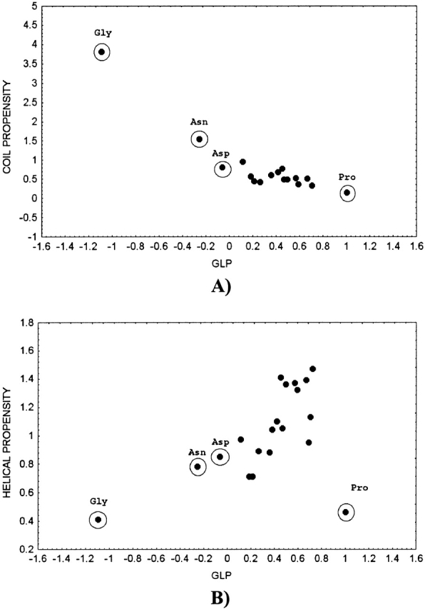
Scatterplot of the generalized local propensity for the 20 amino acids in other-X-other tripeptide, equation 1, versus propensity (Swindells et al. 1995) for coil (A) and α-helical (B) regions of the Ramachandran map.
The coil region covers most of the Ramachandran map. Amino acids that occur in this region frequently, such as Gly, Asn, and Asp, have low GLP because their dihedral angles are distributed over a large area. As the GLP increases, the area occupied by a given amino acid type becomes smaller, and coil propensity decreases (Fig. 1A ▶). The amino acids with positive GLP predominantly occur in the α-helical and/or extended regions, and all have similar low coil propensity, although their GLP may vary. Correlation between the GLP and coil propensity computed for this group of amino acids is therefore low. Pro occurs only in a small area of the extended region and shows the highest GLP and lowest propensity for the coil region. The relationship between the GLP and α-helical propensity is ambiguous, because amino acids with similar α-helical propensities may be distributed differently outside the α-helical region and, as a result, may have significantly different GLP (Fig. 1B ▶).
Residues that demonstrate negative or very small positive values of glp(iXj) do not have a preference for particular areas on the Ramachandran map and thus can adopt a broad range of backbone conformations. We will refer to them as residues with low local coding propensity. Residues that demonstrate large positive values of glp(iXj) do prefer particular areas on the Ramachandran map, and we will refer to them as residues with high local coding propensity. We will use the data obtained in this section to analyze the local coding propensity of SAPs and their flanks by using equations 3 through 5.
SAPs observed in the PDB and their sequence properties
In this section, we identify all types of SAPs observed in the PDB, classify them into five distinct groups based on the types of structure they adopt in two different proteins (Helix-Extended [chameleon fragments]; Helix-Irregular; Extended-Irregular; Irregular-Irregular; and Mixed), and analyze their sequence properties. Table 1 shows the total number of different types of SAPs observed in the PDB. The longest chameleon k-mer observed in the PDB, VLYVKLHN, is eight residues long, and the longest SAPs (KGVVPQLVK and SHHHHHHGS) are nine residues long and belong to the mixed type. It should be noted that EI k-mers are considerably less frequent than are other types. Fragments of sizes 5 and 6 are most frequent, and longer fragments are extremely rare. This observation is consistent with a previous conclusion that sequence fragments greater than size 7 are not well represented in the database of known structures, and there is no prospect for obtaining a large enough database to adequately represent fragments longer than eight residues (Fidelis et al. 1994).
Table 1.
The total number of SAPs found in the PDB
| HEa | HI | EI | II | Mixed | Total | |
| 5-mers | 7310 (8725) | 4818 | 686 | 1387 | 31,190 | 45,391 |
| 6-mers | 373 (465) | 223 | 14 | 53 | 2945 | 3608 |
| 7-mers | 8 (11) | 7 | 0 | 1 | 172 | 188 |
| 8-mers | 0 (1) | 1 | 0 | 1 | 13 | 15 |
| 9-mers | 0 (0) | 0 | 0 | 0 | 2 | 2 |
a The total number of chameleon k-mers (HE) including NMR structures, is shown in parentheses.
Figure 2 ▶ shows the average amino acid frequencies computed for each type of SAP. HE and HI k-mers contain the largest fraction of strong helix (Ala, Leu, Glu, Gln) and sheet formers (Leu, Val, Ile), and the lowest fraction of residues with high coil propensity (Gly, Pro, Asn, and Asp). We define the following groups of amino acids: strong α-helix formers with low β-sheet propensity (Ala, Arg, Glu, and Gln), strong β-sheet formers with low α-helical propensity (Val, Ile, Phe, and Tyr), and amino acids with high propensity for irregular conformation (Gly, Pro, Asn, and Asp). An analysis of the frequency of occurrence of residue pairs shows that the majority of chameleon k-mers (77.2% of all hexamers) have at least one pair consisting of a helix former with low sheet propensity and a sheet former with low helix propensity (Fig. 3 ▶). Among all types of SAPs, chameleon k-mers also have the lowest fraction of pairs consisting of a helix former and a coil former, or a sheet former and a coil former.
Figure 2.

The average amino acid composition of structurally ambivalent peptides.
Figure 3.

The fraction of correlated residue pairs observed in SAPs. The amino acids are partitioned into three groups: helix, strong helix/low sheet propensity; sheet, strong sheet/low helix propensity; and coil, residues with strong coil propensity. See text for details.
The comparison of amino acid frequencies provides a qualitative, rather than a quantitative, description of SAPs. We obtain quantitative estimates of sequence properties by using intrinsic propensities (GLP, α-helix and β-sheet propensities). SAPs can be arranged in the following order based on their average GLP: chameleon k-mers (0.43) → helical-irregular k-mers (0.30) → β-sheet-irregular k-mers (0.153) → irregular-irregular k-mers (0.101). Pairwise comparison of SAP types shows that, with one exception, the average GLP of each type is significantly different from that of other types (p ≤ 10−4) and, therefore, type-specific. The exception is the pair EI-II, which does not show a significant difference in GLP. Among all types of SAPs, the chameleon k-mers have the highest average GLP per residue, 0.43, a value that is higher than the average GLP of all α-helical (0.39) and β-sheet (0.34) fragments observed in the PDB (Table 2). This observation implies that the distribution of dihedral angles associated with trimers found in the chameleon k-mers is narrower than that of average α-helical and, especially, β-sheet fragments. As seen in Table 2, the chameleon k-mers also have high α-helix and β-sheet propensities of the same magnitude, equal to the average secondary structure propensities of all α-helical and β-sheet fragments observed in the PDB. These data indicate that due to a concerted occurrence of strong α-helix and β-sheet formers, as well as lack of amino acids with a strong propensity for areas outside the α-helical and extended regions of the Ramachandran map, chameleon k-mers have a strong preference for both α-helical and β-sheet conformations but not for an irregular conformation.
Table 2.
Average sequence properties of SAPs, their flanking regions and global properties of the protein sequences in which the SAPs were found
| Type of k-mer | GLP (sequence)a | GLP (k-mer)b | α (k-mer)c | β (k-mer)d | GLP (flank)e | α (flank)f | β (flank)g |
| HE (k = 6) | H: 0.30 ± 0.064 | 0.43 ± 0.041 | 1.13 ± 0.121 | 1.13 ± 0.129 | H: 0.58 ± 0.142 | H: 1.02 ± 0.090 | H: 0.99 ± 0.114 |
| E: 0.27 ± 0.071 | E: 0.40 ± 0.156 | E: 0.98 ± 0.084 | E: 0.98 ± 0.102 | ||||
| HI (k = 6) | H: 0.31 ± 0.060 | 0.30 ± 0.056 | 1.08 ± 0.140 | 0.98 ± 0.129 | H: 0.63 ± 0.118 | H: 1.02 ± 0.094 | H: 1.02 ± 0.107 |
| I: 0.27 ± 0.071 | I: 0.53 ± 0.149 | I: 0.98 ± 0.090 | I: 1.00 ± 0.115 | ||||
| EI (k = 5) | E: 0.25 ± 0.076 | 0.15 ± 0.101 | 0.96 ± 0.151 | 1.02 ± 0.151 | E: 0.42 ± 0.130 | E: 0.98 ± 0.093 | E: 1.0 ± 0.11 |
| I: 0.28 ± 0.063 | I: 0.53 ± 0.157 | I: 1.0 ± 0.096 | I: 1.0 ± 0.12 | ||||
| II (k = 6) | 0.28 ± 0.050 | 0.10 ± 0.128 | 0.91 ± 0.169 | 0.87 ± 0.136 | 0.62 ± 0.123 | 1.0 ± 0.095 | 1.02 ± 0.120 |
| Average α-helixh | 0.39 ± 0.037 | 1.12 ± 0.123 | 1.04 ± 0.136 | 0.62 ± 0.120 | 1.02 ± 0.095 | 1.00 ± 0.114 | |
| Average β-sheeth | 0.34 ± 0.046 | 1.03 ± 0.117 | 1.14 ± 0.144 | 0.42 ± 0.144 | 0.99 ± 0.087 | 0.98 ± 0.107 | |
| Average irregularh | 0.21 ± 0.082 | 0.94 ± 0.137 | 0.92 ± 0.142 | 0.57 ± 0.136 | 1.00 ± 0.093 | 1.01 ± 0.111 |
Data for flanking regions of length 6. Each cell that contains two rows of numbers shows data for two alternative conformations of the k-mer pairs: H, data for k-mers in helical conformation; E, data for k-mers in β-sheet conformation; and I, data for k-mers in irregular conformation.
a The average generalized local propensity (equation 2) computed for the entire protein sequence in which the k-mer was found.
b The average generalized local propensity (equation 2) per k-mer.
c The average α-helical propensity per k-mer.
d The average β-sheet propensity per k-mer.
e The average generalized local propensity in k-mer flanks (equation 5).
f The average α-helical propensity in k-mer flanks (equation 5).
g The average β-sheet propensity in k-mer flanks (equation 5).
h The average values computed for all α-helical, β-sheet, and irregular 6-mers observed in the PDB. α-Helical and β-sheet propensities were taken from Swindells et al. (1995). In each cell, pairs of values that show a significant difference (two-sample t test P < 0.01) are shown in boldface type.
We next ask how different the amino acid composition of SAPs is from that observed in the nonredundant PDB database as a whole? A direct comparison of the amino acid composition of SAPs and the average composition in the PDB unavoidably leads to a bias caused by the difference between the average composition in the PDB and the composition specific to a given type of secondary structure (α-helix, β-sheet, or irregular). To avoid this bias, we compare the amino acid composition of SAPs with that of fragments with corresponding secondary structure. For instance, the composition of chameleon k-mers was compared with the average composition of α-helical and β-sheet k-mers of the same length. The results of this comparison are shown in Figure 4 ▶. It will be seen that each type of SAP has a specific amino acid composition, and those compositions generally conform to empirical expectation:
Chameleon k-mers contain more hydrophobic strong sheet and helix formers than does the average α-helical k-mer. They also contain more Ala and Leu and more of the hydrophilic helix-former Glu than does the average β-sheet.
Helix-irregular k-mers have helical propensity that is higher than the average for irregular k-mers and lower than the average for helical k-mers. Compared with the average helical k-mer, they contain a large excess of the conformationally flexible amino acid Gly and a higher percentage of the sheet formers Val and Thr. They also contain more of the hydrophobic helix-formers Ala and Leu and the β-sheet-former Val, as well as less Pro than the average irregular k-mer. Overall, the composition of HI k-mers lies between those of helical and irregular fragments, which may facilitate the transition between helical and irregular conformations in these k-mers.
Extended-irregular k-mers have β-sheet propensity that is higher than the average for irregular k-mers and lower than the average for β-sheet k-mers. They also contain more helix formers and fewer β-sheet formers and amino acids with strong preference for coil conformation than does the average β-strand or irregular fragments. Increased helical propensity may facilitate the transition between the extended conformation and more compact irregular conformations.
Figure 4.
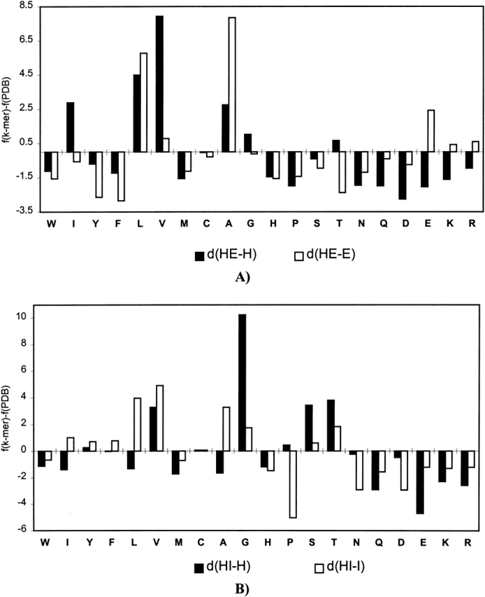
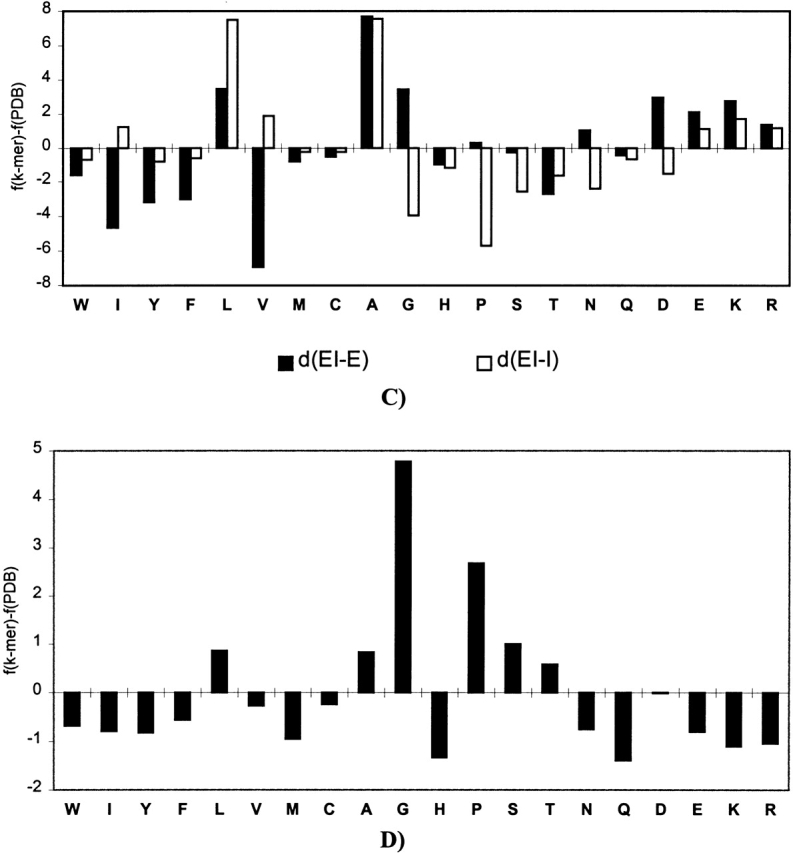
The difference between amino acid composition of the PDB and the average amino acid composition of the SAPs found in the PDB. For each amino acid type ai, the difference between fk-mer(j)(ai) − fPDB(m)(ai) is shown, where fk-mer(j)(ai) is the average frequency of ai in k-mers of type j, and fPDB(m)(ai) is the frequency of ai in all k-mers of conformation m found in the PDB. Positive values indicate an excess of ai in SAPs compared with the average amino acid composition of conformation m in PDB. d(HE-H) and d(HE-E) indicate the difference between the average composition of k-mers of type HE and the average composition of helical, H, or β-strand, E, fragments; d(HI-H) and d(HI-I) indicate the difference between type HI and the average composition of helical, H, or irregular, I, fragments; d(EI-E) and d(EI-I) indicate the difference between type EI and the average composition of β-strand, E, or irregular, I, fragments; and d(I-I) indicates the difference between type II and the average composition of irregular fragments. The data shown is for hexamers (pentamers in the case of EI type).
Irregular-irregular k-mers show the lowest local coding propensity and contain a large excess of Gly and Pro. Gly is the most conformationally flexible amino acid and provides extra degrees of freedom to the backbone. Pro is the least flexible amino acid, and its function in this context may be to compensate partially for an excess of conformational entropy provided by Gly.
Irregular k-mers in our classification include turns ("T" in the DSSP assignment). In many cases, residues in turn conformation (such as type II turns) are located in the helical region of the Ramachandran map and thus have (φ,ξ) angles similar to those of helical residues. Automatic secondary structure classification may erroneously assign the turn conformation to short helices or vice versa. We therefore need to check whether k-mers of HI type in irregular conformation contain a high percentage of turns. We compare the secondary structure content of HI, EI, and II k-mers in the irregular conformation. Surprisingly, HI k-mers have the lowest percentage of residues in turn conformations and the largest percentage in the coil state (unclassified conformation in the DSSP assignment). This observation confirms that HI k-mers indeed undergo a helix → coil conformational transition.
The SAPs can be arranged in order of increasing average sequence complexity, Q (equation 6), as follows: HE (Q = 3.79) → II (Q = 3.87) → EI (Q = 3.91) → HI (Q = 3.95). The average sequence complexity of the data set from which the SAPs was sampled is 4.19. The observation that all types of SAP have sequence complexity below average, and are constructed using a limited number of "preferred" residues, implies that the number of different short flexible k-mers (especially of chameleon k-mers, which have the lowest sequence complexity) should be limited. We check this assumption by asking how many longer chameleon k-mers can be identified by matching to shorter ones. We used a selection method based on local sequence alignment provided by the PISCES Web site (see Materials and Methods) to construct a nonredundant subset of PDB structures (both high-resolution X-ray and NMR structures) such that all proteins in this subset have pairwise sequence identity <50%. All k-mers with chameleon properties were identified in this subset. The nonredundant nature of this subset ensures that all SAPs, regardless of their length, are separated from each other by a significant evolutionary distance. Matching known chameleon 5-mers against 6-mers (only exact matches were considered) shows that 68% of all chameleon 6-mers from our data set are identified. Similarly, 91% of all 7- and 8-mers in our data set are identified by matching them against 5- and 6-mers. These results indicate that the repertoire of chameleon k-mers is indeed limited to certain combinations of residues, and during the course of protein evolution, longer k-mers are constructed by adding a few residues with appropriate local propensity to shorter ones (or, conversely, that shorter k-mers are constructed by trimming a few residues from longer ones).
Factors that may affect the conformational preferences of SAPs
The amino acid composition of SAPs allows them to adopt at least two different backbone conformations. We now ask what factors govern conformational choice in these peptides. To gain insights into this problem, we analyze secondary structure content, solvent accessibility, and local structural propensity in the flanking regions of SAPs, as well as the overall properties of protein sequences in which SAPs were found. Our goal is to find out whether each of two alternative conformations of a given type of SAP is associated with specific properties of its flanking regions (local context) or of the entire sequence (global context).
To compare the local sequence and structural context of two alternative conformations of the same SAP, we first need to determine how many adjacent residues we must take into account. To do this, we compared average local propensity, solvent accessibility, and secondary structure content computed for flanking windows of size 4 as a function of the sequence separation between the k-mer and the windows (equation 4). The results of this comparison for the GLP and solvent accessibility are shown in Figures 5 and 6 ▶ ▶. The difference in local propensity and solvent accessibility between flanks of two distinct conformations of the same SAP rapidly decreases to zero when sequence separation reaches four to six residues. It should be remarked, however, that we did not find a significant difference in hydrophobic properties between flanks of two conformations of the same SAP. The difference in α-helical and β-sheet propensity decays to zero faster than that in the GLP (data not shown). The difference in secondary structure content also rapidly decreases (data not shown) and reaches the average difference (Table 3) observed between two groups of proteins that contain distinct conformations of the same SAP type. The length of flanking regions that maximizes the average difference between two distinct conformations of the same SAP type is six residues.
Figure 5.

The difference in the average generalized local propensity (GLP) between flanking regions of two distinct conformations, 1 and 2, of the same k-mer pair as a function of sequence separation, s, from a flanking window of size 4 (w = 4) to the ends of the k-mer. Equation 5 was used to compute the average GLP of the flanks in each conformation. For HE k-mers, conformation 1 is helix, conformation 2 is β-sheet, and k = 6. For HI k-mers, 1 is helix, 2 is irregular, and k = 6. For EI k-mers, 1 is β-sheet, 2 is irregular, and k = 5. All non-zero differences shown are statistically significant (two-sample t test P < 0.05).
Figure 6.

The difference in the average normalized solvent accessibility (NSA), between flanking regions of two distinct conformations, 1 and 2, of the same SAP type as a function of sequence separation, s, from flanking window of size 4 (w = 4) to the ends of k-mer. Equation 5 was used to compute the average NSA of the flanks in each conformation. Notation is the same as in Figure 5 ▶.
Table 3.
The average secondary structure content of the flanking regions of SAPs and the protein sequences in which the SAPs were found
| Type of k-mer | Group 1 (flanks)a | Group 2 (flanks)b | Group 1 (sequence)a | Group 2 (sequence)b |
| HE (k = 6) | H: 67.79 ± 21.45 | H: 7.75 ± 12.92 | H: 49.76 ± 16.64 | H: 24.33 ± 14.80 |
| E: 2.76 ± 7.68 | E: 37.09 ± 20.86 | E: 13.15 ± 10.03 | E: 33.24 ± 13.74 | |
| T: 10.56 ± 10.54 | T: 17.77 ± 12.67 | T: 11.05 ± 2.93 | T: 11.65 ± 2.85 | |
| S: 5.65 ± 7.97 | S: 12.81 ± 11.54 | S: 7.49 ± 2.94 | S: 9.30 ± 2.73 | |
| C: 12.60 ± 11.96 | C: 23.31 ± 15.13 | C: 17.61 ± 4.54 | C: 20.19 ± 4.55 | |
| HI (k = 6) | H: 68.67 ± 22.78 | H: 18.00 ± 23.50 | H: 49.59 ± 16.12 | H: 31.52 ± 15.63 |
| E: 4.79 ± 10.11 | E: 21.21 ± 23.79 | E: 13.18 ± 9.08 | E: 21.00 ± 11.76 | |
| T: 8.67 ± 11.23 | T: 15.08 ± 13.03 | T: 11.02 ± 3.00 | T: 12.57 ± 3.37 | |
| S: 5.75 ± 7.67 | S: 11.75 ± 11.46 | S: 7.52 ± 2.97 | S: 10.07 ± 3.33 | |
| C: 11.42 ± 11.22 | C: 30.62 ± 17.48 | C: 17.74 ± 4.79 | C: 22.99 ± 6.11 | |
| EI (k = 5) | H: 8.90 ± 14.33 | H: 23.44 ± 24.74 | H: 23.62 ± 16.01 | H: 33.24 ± 16.34 |
| E: 42.30 ± 22.66 | E: 25.20 ± .66 | E: 34.04 ± 14.87 | E: 21.28 ± 13.12 | |
| T: 15.83 ± 12.91 | T: 13.59 ± 14.26 | T: 11.51 ± 2.88 | T: 12.65 ± 3.00 | |
| S: 11.53 ± 11.43c | S: 11.17 ± 12.01c | S: 9.26 ± 2.81 | S: 10.03 ± 3.27 | |
| C: 20.37 ± 14.78 | C: 24.62 ± 17.34 | C: 20.26 ± 4.84 | C: 21.47 ± 5.08 | |
| II (k = 6) | H: 20.83 ± 26.80 | H: 30.06 ± 17.47 | ||
| E: 25.52 ± 27.26 | E: 22.05 ± 11.78 | |||
| T: 11.81 ± 10.85 | T: 12.53 ± 3.31 | |||
| S: 8.68 ± 10.31 | S: 10.36 ± 3.15 | |||
| C: 30.73 ± 19.84 | C: 23.34 ± 5.90 |
Data for flanking regions of length 6. In each cell, letters denote the type of secondary structure in the DSSP classification: H, helix; E, β-sheet; T, turn; S, abrupt change in chain direction; and C, coil (not classified).
a Group 1 shows the data for helical conformation of k-mer pair of type HE, HI and the data for β-sheet conformation of k-mer pairs of type EI.
b Group 2 shows the data for the β-sheet conformation of k-mer pairs of type HE and irregular conformation of k-mer pairs of type HI and EI.
c The difference in secondary structure contents between two conformations of each SAP is statistically significant for all classes of secondary structure (two-sample t test P < 0.01), except for S in flanks of EI k-mers.
The average differences in local and global sequence context between two conformations of the same SAP type are shown in Figures 7 and 8 ▶ ▶ and Tables 2 through 4 and can be summarized as follows:
The flanks of chameleon k-mers in helical and sheet conformation show the largest difference in local propensity. The flanks of chameleon k-mers in the helical conformation contain an excess of hydrophobic and hydrophilic helix formers and have a high local coding propensity. In most cases, these flanks also have helical conformation (68% of the time). The flanks of chameleon k-mers in the β-sheet conformation contain an excess of conformationally variable residues (Gly, Asp, Asn) and Pro and only a moderate excess of residues with strong β-sheet propensity. As a result, flanks of chameleon k-mers in the β-sheet conformation have a low local coding propensity. Flanking residues are in the β-sheet conformation only ∼37% of the time. Additional information about the local context of chameleon fragments can be obtained by analyzing how often they occur in the middle of helix or β-sheet. We define a fragment as being located in the middle of a regular secondary structure if at least two residues immediately adjacent to both ends of the fragment have the same regular structure. Chameleon hexamers in the helical conformation are located in the middle of a helix 59% of the time, whereas only 15% of chameleon hexamers in the β-sheet conformation are located in the middle of a β-sheet. We conclude that strong local helical propensity in the flanking residues forces chameleon k-mers to adopt a helical conformation. In the absence of flanks with high local coding propensity, chameleon k-mers adopt the more energetically favorable extended conformation. A factor of lesser importance may be interaction with solvent: The chameleon k-mers in the helical conformation are more accessible to solvent, whereas their flanking residues are less accessible than those in the β-sheet conformation. The chameleon k-mers in both conformations are slightly less accessible than are average helical and sheet fragments. However, it should be noted that the flanks of chameleon k-mers in the helical conformation do not show unusual properties. Their average local propensity and solvent accessibility are similar to those observed in flanks of all helical fragments in general (Tables 2, 4).
The flanks of k-mers of helix-irregular type show the highest local coding propensity and the most significant difference in amino acid composition. HI k-mers in the helical conformation are flanked by residues with high helical propensity, whereas in irregular conformation, they are flanked by conformationally flexible residues and Pro. The final conformation of these k-mers also appears to be significantly modulated by solvent interactions (Table 4). It is reasonable to assume that because of a low propensity for β-sheet conformation, when HI k-mers are placed into a sequence context with low local coding propensity, they adopt irregular conformation. HE k-mers in similar context adopt the energetically favorable extended conformation.
The flanks of EI k-mers in the β-sheet conformation have low coding propensity and show a moderate excess of conformationally flexible residues. These k-mer pairs also show the largest difference in solvent accessibility (Table 4). Because these k-mers have an average β-sheet propensity higher than that of irregular fragments, one may assume that upon burial in a sequence context with low local coding propensity, EI k-mers tend to adopt the extended conformation and form hydrogen bonds with complementary β-strands, whereas when accessible to solvent and flanked by residues with high local coding propensity, they tend to adopt irregular conformations.
The strongest local propensity in flanking regions is observed for irregular-irregular k-mers, which exhibit the highest degree of backbone variability and require strong conformational restrictions on their flanks in order to be fixed in a stable conformation.
Figure 7.

The difference in the average amino acid composition, f(i|m) − f(i|n), between flanking regions of two distinct conformations, m and n, of the same SAP type. f(i|m) is the average frequency of amino acid i in the flanks of the conformation m. HE, m = H and n = E; HI, m = H and n = I; and EI, m = E and n = I. The data shown is for hexamers (pentamers in the case of EI type) and for flanks of length 6.
Figure 8.

Clustering tree that shows the similarity between flanking regions of k-mers in helical, sheet, and irregular conformations. The distances between flanking regions are computed by using equation 7. HE (HI) in helix indicates SAPs of HE (HI) type in helical conformation; HE (EI) in sheet, SAPs of HE (EI) type in sheet conformation; and EI (HI) in irregular, SAPs of EI (HI) type in irregular conformation. All helix, sheet, and irregular indicates the average frequencies in flanks of all helical, sheet, and irregular k-mers observed in the PDB.
Table 4.
The average normalized solvent accessibility (NSA) per residue in SAPs and their flanking regions
| Type of k-mer | Fragment NSA | Flank NSA |
| HE (k = 6) | H: 0.19 ± 0.121 | H: 0.27 ± 0.107 |
| E: 0.16 ± 0.124 | E: 0.32 ± 0.100 | |
| HI (k = 6) | H: 0.21 ± 0.129 | H: 0.25 ± 0.105 |
| I: 0.37 ± 0.175 | I: 0.28 ± 0.128 | |
| EI (k = 5) | E: 0.15 ± 0.130 | E: 0.29 ± 0.102 |
| I: 0.31 ± 0.162 | I: 0.24 ± 0.113 | |
| Average α-helix (k = 6) | 0.21 ± 0.122 | 0.27 ± 0.109 |
| Average β-sheet (k = 6) | 0.14 ± 0.117 | 0.31 ± 0.103 |
| Average irregular (k = 6) | 0.36 ± 0.163 | 0.27 ± 0.123 |
Data for flanking regions of length six. Each cell with two rows shows the data for two alternative conformations of SAP: H, the data for SAPs in helical conformation; E, the data for SAPs in β-sheet conformation; and I, the data for SAPs in irregular conformation. Within each cell, the difference between two conformations of the same SAP type is statistically significant (two-sample t test P < 0.01).
Note that a statistically significant difference in local coding propensity between flanking regions of two alternative conformations of the same SAP is observed for all types of SAPs (Table 3). Do the flanks of SAPs possess any special properties compared to the properties of average fragments? A cluster analysis of the flanks of SAPs and all helical, sheet, and irregular fragments shows that all fragments with the same conformation have similar conformation-specific local sequence context (Fig. 8 ▶). This implies that the average local sequence context of SAPs is similar to the average local context of all peptides with corresponding conformation and therefore is not unusual. The difference in global properties of protein sequences that contain alternative conformations of the same SAP is similar to that of the flanking regions, but much less marked (Table 2; Fig. 9 ▶). An analysis of secondary structure content also shows that the difference in local structural context is more marked than that in the global one (Table 3). However, the difference in global secondary structure content should not be underestimated. For instance, proteins that contain a SAP (HE or EI) in a β-sheet conformation have the highest average β-sheet and lowest helical content among all groups studied. It should also be remarked that a significant difference, both in global and local structural context, between two alternative conformations of the same type of SAPs is observed for all types of local structure, regular and irregular (Table 3).
Figure 9.

The difference in the average global amino acid composition, f(i|m) − f(i|n), between sequences that contain two distinct conformations, m and n, of the same SAP type. The notation is the same as in Figure 7 ▶. The Y-axis is drawn to the same scale as that in Figure 7 ▶.
Discussion
The results of this study show that SAPs observed in known protein structures cover a broad range of conformations, both regular and irregular, and all possible types of conformational pairs: helix–sheet, helix–coil, sheet–coil, and coil–coil. Local propensity, tuned by selection of appropriate amino acids, is the principal factor that differentiates SAPs from average fragments with corresponding secondary structure. These data support the empirical assumptions that SAPs have strong intrinsic propensities for at least two types of local conformation and are likely to fluctuate in equilibrium between these two conformations, and that they require a minimum of external factors to choose the one most suitable for given structural context (Young et al. 1999).
What features of protein environment modulate the final conformation of a SAP? A significant difference between two distinct conformations of the same SAP is observed both in the overall sequence and structural properties of the proteins harboring the SAP (global context) and in the sequence and structural properties of its flanking regions (local context), as well as in the per-fragment and per-flank pattern of solvent accessibility. The importance of the global protein environment in determining the final conformation of SAPs has been pointed out previously (Cohen et al. 1993). The data reported here indicate that local sequence context is another major determinant of the final conformation of these fragments, with solvent accessibility also playing an important role, especially in the case of irregular conformations. These data do not support the earlier conclusion that most SAPs have similar patterns of solvent accessibility (Cohen et al. 1993). A likely explanation of this disagreement is that previous studies were performed on a much smaller data set (59 hexapeptides), which did not allow observation of fine differences. The amino acid composition and local propensity of flanking regions of SAPs are similar to those of average fragments (Fig. 8 ▶, Table 2). This observation indicates that there exist general conformation-specific signals in the local context of all helical, sheet, and irregular fragments that can be used in structure prediction to distinguish between alternative conformations of the same SAP. The difference in local context between alternative conformations of most SAPs becomes statistically insignificant for residues separated by more than 6 to 10 positions from the SAP. Many secondary structure prediction methods use six to eight adjacent residues to predict conformation for the central residue (Rost and Sander 1994; Garnier et al. 1996) and therefore seem to extract nearly the maximal possible amount of information from local sequence context. However, it is worth noting that in the case of EI k-mers, a significant difference in local propensity and solvent accessibility of flanking regions is observed up to 11 adjacent residues. This indicates that a larger window size is required in order to capture all the contextual differences between β-sheet and irregular conformations.
Our results indicate that both local and global context modulate the final conformation of SAPs. What is the relative contribution of each of these factors during the folding process? It is reasonable to assume that when a HE or HI k-mer is flanked by strong helix formers, it undergoes a fast cooperative transition to an α-helical conformation initiated by adjacent residues, which may adopt native-like helical conformation during the early stages of protein folding (Baldwin and Rose 1999). Low β-sheet content in a mainly α protein or in a mainly α-helical domain of an α/β protein may facilitate this process, because of the absence of complementary β-strands that might form long-range hydrogen bonds with the SAP and interfere with helix formation. On the other hand, a HE or EI k-mer located in a sequence context with low local coding propensity may adopt the energetically favorable extended conformation. The greater conformational flexibility in flanks that we observe in this case may allow the k-mer to find a complementary β-strand in a protein with high β-sheet content, and form long-range hydrogen bonds. These assumptions are consistent with experimental data of Minor Jr. and Kim (1996) and the results of folding simulations performed by Baldwin and Rose (1999), which showed that a chameleon fragment of length 11 adopts a helical conformation when placed in the helical context within protein G, and the same fragment adopts a β-sheet conformation when placed in the β-sheet context within the same protein.
The results presented in this work were obtained by using a set of relatively short SAPs observed in a data set of soluble globular proteins that represent the majority of proteins available in the PDB. There is a growing body of evidence indicating that many proteins, especially from eukaryotes, contain long flexible disordered fragments (Wright and Dyson 1999; Dunker et al. 2002; Liu et al. 2002), which are not well represented in the PDB (Huntley and Golding 2002). Elucidation of the rules governing the behavior of these long disordered fragments requires additional theoretical and experimental study.
Materials and methods
Local conformational variability of the central residue in a tripeptide
To determine the degree of context-dependent conformational variability of each of the 20 amino acids, we analyze the width of the distribution of (φ,ξ) angles associated with the central amino acid in a tripeptide iXj. The central residue, X, is described by a full 20-letter alphabet, whereas the flanking residues i and j are collapsed into three groups, based on their side chain properties: group 1, Gly; group 2, Pro; and group 3, 18 other amino acids.
Division into a larger number of groups is not statistically feasible, given the current size of the data set of nonredundant structures. Gly and Pro were separated from the rest of the amino acids because this grouping of the amino acids was shown to be the most informative three-letter alphabet for defining local sequence/structure relationships in proteins (Solis and Rackovsky 2000, 2002). Our approach is an extension of a method based on the comparison of the entropy of structural distributions in the virtual-bond backbone representation (Rackovsky 1990), which was used to identify tetramers that encode for identifiable distributions of local structure (Rackovsky 1993).
The Ramachandran plot was divided by using an equally spaced four-by-four grid (−180° to −90°, −90° to 0°, 0° to 90°, and 90° to 180° on both axes). The width of the distribution of dihedral angles for an amino acid X in a given tripeptide iXj is measured by its entropy (Rackovsky 1990, 1993) by using the following equation:
 |
(1) |
 |
where S(iXj) is the observed Shannon entropy of the tripeptide-specific distribution of dihedral angles; n is the total number of grid cells used to partition the Ramachandran map (n = 16 here); p(k) is the fractional frequency of occurrence of tripeptide iXj in the grid cell k; NiXj is the number of occurrences of tripeptide iXj in the data set; and SR(NiXj) is the average entropy of a distribution of NiXj tripeptides randomly sampled without replacement from the data set.
To compute the average entropy for each tripeptide iXj, we generate 105 random samples of size NiXj (a number sufficient to ensure convergence to three decimal digits). Comparison to a reference random distribution of the same size as the observed number of tripeptides provides an automatic correction for the unequal number of observations and unequal proportion of residues observed in helical and extended conformations (Rackovsky 1993; Swindells et al. 1995). A positive value of glp(iXj) indicates that the average entropy of random distributions is greater than that observed for a given tripeptide iXj. This implies that the tripeptide is preferentially observed in specific areas of the Ramachandran plot. Negative values of glp(iXj) correspond to a lack of preference of the tripeptide iXj for specific values of φ and ξ angles. The higher the value of glp(iXj), the smaller the area on the Ramachandran plot the tripeptide is observed to occupy. It should be emphasized that for each amino acid, this approach measures the context-dependent breadth of the allowed area on the Ramachandran map, not a preference for particular values of the dihedral angles. The latter property is measured by secondary structure propensities. glp(iXj) combines information about preferences for α-helical, β-sheet, and coil regions into one "flexibility" index. We will refer to this index as the GLP. When we refer to conformational variability of a particular amino acid type, we will imply the context-dependent degree of backbone conformational variability given by equation 1. It should be remarked that the resolution of the GLP can be increased, as the size of the data set increases, by partitioning the amino acid alphabet into a larger number of groups and/or dividing the Ramachandran map using a finer grid.
The GLP can be used to compute the average conformational variability index of a sequence fragment, GLP(S):
 |
(2) |
where L is the sequence length and Am is amino acid in sequence position m.
To derive tripeptide-specific distributions of dihedral angles, we used a nonredundant data set of high-resolution X-ray structures, with resolution ≤3.0 Å, R-factor ≤0.3, and sequence length ≥40 residues, such that all chains have pairwise sequence identity <20%. The data set consists of 1647 structures (389,120 tripeptides) and was obtained from the PISCES Web site (http://www.fccc.edu/research/labs/dunbrack/pisces/), which provides the most up-to-date compilation of the nonredundant PDB database by using the selection method of Hobohm et al (1993). The (φ,ξ) angles were computed by using the DSSP program (Kabsch and Sander 1983). A complete set of generalized local propensities is available online at http://c3.biomath.mssm.edu/~igor/trimers.txt.
Identification of SAPs
We selected from the PDB (Berman et al. 2000) all pairs of high-resolution X-ray structures (resolution ≤3.0 Å, R-factor ≤0.3, and length ≥40 residues) that have pairwise sequence identity <50%. Transmembrane fragments annotated in the SCOP structural database (Murzin et al. 1995) were excluded from the analysis. Each pair was scanned for sequentially identical peptide pairs (SIPPs), and we retain only those SIPPs that exist in two distinct backbone conformations. SIPPs with two distinct backbone conformations were identified by using the following two-step procedure:
All positions with matching regular secondary structure (helix–helix or strand–strand) were eliminated from each SIPP. Fragments shorter than five residues were ignored. This greatly reduces the CPU time required to perform structural superposition of all fragments. For each SIPP step, one produces a set of one or more pairs of conformations.
Pairs of conformations obtained in step 1 are optimally superimposed, and only those pairs are retained which have a Cα root mean square deviation (RMSD) above a certain threshold. Two conformations of the same sequence fragment are considered to be significantly different if their Cα RMSD is equal to or greater than the average RMSD of an ensemble of random fragments of the same length. We will refer to a sequence fragment that exists in two dissimilar conformations in two different proteins as a SAP.
To obtain the dissimilarity threshold, we compute the average Cα RMSD for randomly selected pairs of structural fragments of length 5 to 15 (using 105 random pairs for each fragment length). Only those pairs are used that come from two different proteins and do not have positions with matching regular secondary structure. Random pairs were selected from the September 2001 release of the PDB_SELECT data set of nonredundant high-resolution X-ray structures clustered at 25% sequence similarity (Hobohm et al. 1993), without chain breaks, with resolution ≤2.0 Å, and R-factor ≤0.2 (471 proteins in total). Cα RMSDs were computed by using the ProFit program (Martin 2001). Secondary structure was assigned by using the DSSP program (Kabsch and Sander 1983).
If a fragment of length k in protein r had a crystallographic B-factor 2 SD above the average B-factor computed for all fragments of length k in the protein r, this fragment was excluded from the analysis. This approach allows one to remove poorly characterized fragments by taking into account a protein-specific dependence of B-factor on the particular method used to refine crystallographic data (Saqi 1995).
All final SAPs were classified in five nonredundant categories based on secondary structure: (1) HE, the SAP exists as a helix in the DSSP assignment in one protein and a β-sheet in the other; (2) HI, the SAP exists as a helix in one protein and in an irregular conformation (S, T, B, or C in the DSSP assignment) in the other; (3) EI, the SAP exists as a β-sheet in one protein and in an irregular conformation in the other; (4) II, the SAP exists in different irregular conformations in the two proteins; and (5) mixed, all SAPs that can not be classified into the first four groups.
We will refer to these SAPs as k-mer pairs (pentamers, hexamers, etc.), denoting sequence fragments of length k that exist in two significantly different conformations in distinct proteins. It should be emphasized that the SAPs were classified based solely on the structural criteria outlined above, without regard to their amino acid composition. We also generated an extended list of chameleon k-mers by including NMR structures and selecting SAPs that exist as a helix in one protein and a β-sheet in the other. The data set of all SAPs used in this work is available upon request.
For a given amino acid property, P (index P denotes a particular property, such as helical or sheet propensity), the average property of a k-mer of type i found in conformation c in protein r, is computed by using the following equation:
 |
(3) |
The average property in flanking regions of a k-mer of type i, found in conformation c in protein r, is computed by using the following equation:
 |
(4) |
where w is the length of flanking regions; j is the sequence position of the first residue in the k-mer; k is the size of the k-mer; s is the sequence separation between the k-mer and flanking regions (s = 0 means that the flanking region is immediately adjacent to the k-mer); Arl is the amino acid at sequence position l of protein r; and P(Arl) is the value of property P for this amino acid. In the case of the GLP, Arl is a tripeptide centered at sequence position l, and P(Arl) is the GLP of this tripeptide, glp(Arl). If for some k-mer (j-w-s) ≤ 0 or (j+s+k+w-1) > Lr (where Lr is the length of protein r), that k-mer was excluded from the computation of the properties of flanking regions.
The average property P computed over flanks of all k-mers of type i found in conformation c is given by
 |
(5) |
where N(i,c) is the number of proteins that contain the k-mer of type i in conformation c. The average property computed over all k-mers of type i found in conformation c, <Pk-mer(i|c)>, is computed in a similar fashion. We used the conventional α-helical and β-sheet propensities of amino acids taken from Swindells et al. (1995) to determine the average α-helical and β-sheet propensities of a sequence fragment by means of equations 3 through 5.
Entropic sequence complexity of a sequence fragment, Q(S), was computed by using the following equation (Wotton 1993):
 |
(6) |
where fi is the normalized frequency of amino acid type i in sequence S.
We use the UPGMA method (average linkage; Sneath and Sokal 1973) to cluster groups of sequence fragments according to their average amino acid frequencies. The output of the method is a clustering tree that shows the degree of similarity between these groups. The distance between a group of sequence fragments of type i and a group of sequence fragments of type j is defined as follows:
 |
(7) |
where fik is the average normalized frequency of amino acid type k in group i.
Acknowledgments
This work was supported by grant number 1R01 LM06789 from the National Library of Medicine of the NIH. We are grateful to Dr. Armando Solis for helpful discussions. The publication costs of this article were defrayed in part by payment of page charges. This article must therefore be hereby marked "advertisement" in accordance with 18 USC section 1734 solely to indicate this fact.
Article and publication are at http://www.proteinscience.org/cgi/doi/10.1110/ps.03209703.
References
- Argos, P. 1987. Analysis of sequence-similar pentapeptides in unrelated protein tertiary structures: Strategies for protein folding and a guide for site-directed mutagenesis. J. Mol. Biol. 197 331–348. [DOI] [PubMed] [Google Scholar]
- Bahar, I., Kaplan, M., and Jernigan, R.L. 1997. Short-range conformational energies, secondary structure propensities, and recognition of correct sequence-structure matches. Proteins 29 292–308. [DOI] [PubMed] [Google Scholar]
- Baldwin, R.L and Rose, G.D. 1999. Is protein folding hierarchic? I: Local structure and peptide folding. TIBS 24 26–33. [DOI] [PubMed] [Google Scholar]
- Berman, H.M., Westbrook, J., Feng, Z., Gilliland, G., Bhat, T.N., Weissig, H., Shindyalov, I.N., and Bourne, P.E. 2000. The Protein Data Bank. Nucleic Acids Res. 28 235–242. [DOI] [PMC free article] [PubMed] [Google Scholar]
- Bowie, J.U., Luthy, R., and Eisenberg, D. 1991. A method to identify protein sequences that fold into a known three-dimensional structure. Science 253 164–170. [DOI] [PubMed] [Google Scholar]
- Bystroff, C., Thorsson, V., and Baker, D. 2000. HMMSTR: A hidden Markov model for local sequence–structure correlations in proteins. J. Mol. Biol. 301 173–190. [DOI] [PubMed] [Google Scholar]
- Cohen, B.I., Presnell, S.R., and Cohen, F.E. 1993. Origins of structural diversity within sequentially identical peptides. Protein Sci. 2 2134–2145. [DOI] [PMC free article] [PubMed] [Google Scholar]
- Dalal, S. and Regan, L. 2000. Understanding the sequence determinants of conformational switching using protein design. Protein Sci. 9 1651–1659. [DOI] [PMC free article] [PubMed] [Google Scholar]
- Dunker, K.A., Brown, C.J., Lawson, D.J., Iakoucheva, L.M., and Obradovic, Z. 2002. Intrinsic disorder and protein function. Biochemistry 41 6573–6582. [DOI] [PubMed] [Google Scholar]
- Fidelis, K., Stern, P.S., Bacon, D., and Moult, J. 1994. Comparison of systematic search and database methods for constructing segments of protein structure. Protein Eng. 7 953–960. [DOI] [PubMed] [Google Scholar]
- Garnier, J., Gibrat, J.-F., and Robson, B. 1996. GOR secondary structure prediction method version IV. Methods Enzymol. 266 540–553. [DOI] [PubMed] [Google Scholar]
- Gerstein, M. and Krebs, W. 1998. A database of macromolecular motions. Nucleic Acids Res. 26 4280–4290. [DOI] [PMC free article] [PubMed] [Google Scholar]
- Griffiths-Jones, S.R., Sharman, G.J., Maynard, A.J., and Searle, M. 1998. Modulation of intrinsic phi,psi propensities of amino acids by neighboring residues in the coil regions of protein structures: NMR analysis and dissection of a β-hairpin peptide. J. Mol. Biol. 284 1597–1609. [DOI] [PubMed] [Google Scholar]
- Han, K.F. and Baker, D. 1996. Global properties of the mapping between local amino acid sequence and local structure in proteins. Proc. Natl. Acad. Sci. 93 5814–5818. [DOI] [PMC free article] [PubMed] [Google Scholar]
- Hobohm, U., Scharf, M., and Schneider, R. 1993. Selection of representative protein data sets. Protein Sci. 1 409–417. [DOI] [PMC free article] [PubMed] [Google Scholar]
- Huntley, M.A. and Golding, G.B. 2002. Simple sequences are rare in Protein Data Bank. Proteins 48 134–140. [DOI] [PubMed] [Google Scholar]
- Jonassen, I., Eidhammer, I., Grindhaug, S.H., and Taylor, W.R. 2000. Searching the protein structure databank with weak sequence patterns and structural constraints. J. Mol. Biol. 304 599–619. [DOI] [PubMed] [Google Scholar]
- Kabsch, W. and Sander, C. 1983. Dictionary of protein secondary structure: Pattern recognition of hydrogen-bonded and geometrical features. Biopolymers 22 2577–2637. [DOI] [PubMed] [Google Scholar]
- ———. 1984. On the use of sequence homologies to predict protein structure: Identical pentapeptides can have different conformations. Proc. Natl. Acad. Sci. 81 1075–1078. [DOI] [PMC free article] [PubMed] [Google Scholar]
- Kuznetsov, I.B. and Rackovsky, S. 2002. Discriminative ability with respect to amino acid types: Assessing the performance of knowledge-based potentials without threading. Proteins 49 266–284. [DOI] [PubMed] [Google Scholar]
- Kwasigroch, J.-M., Chomilier, J., and Mornon, J.-P. 1996. A global taxonomy of loops in globular proteins. J. Mol. Biol. 259 855–872. [DOI] [PubMed] [Google Scholar]
- Liu, J., Tan, H., and Rost, B. 2002. Loopy proteins appear conserved in evolution. J. Mol. Biol. 322 53–64. [DOI] [PubMed] [Google Scholar]
- Martin, A.C.R. 2001. ProFit V2.2. http://www.bioinf.org.uk/software/profit/
- Mezei, M. 1998. Chameleon sequences in PDB. Protein Eng. 11 411–414. [DOI] [PubMed] [Google Scholar]
- Minor Jr., D.L. and Kim, P.S. 1996. Context-dependent secondary structure formation of a designed protein sequence. Nature 380 730–734. [DOI] [PubMed] [Google Scholar]
- Murzin, A.G., Brenner, S.E., Hubbard, T., and Chothia, C. 1995. SCOP: A structural classification of protein database for the investigation of sequence and structures. J. Mol. Biol. 247 536–540. [DOI] [PubMed] [Google Scholar]
- Prusiner, S. 1998. Prions. Proc. Natl. Acad. Sci. 95 13363–13383. [DOI] [PMC free article] [PubMed] [Google Scholar]
- Rackovsky, S. 1990. Quantitative organization of known protein X-ray structures, I: Methods and short-length scale results. Proteins 7 378–402. [DOI] [PubMed] [Google Scholar]
- ———. 1993. On the nature of the protein folding code. Proc. Natl. Acad. Sci. 90 644–648. [DOI] [PMC free article] [PubMed] [Google Scholar]
- Romero, P., Obradovic, Z., Li, X., Garner, E.C., Brown, C.J., and Dunker, A.K. 2001. Sequence complexity of disordered proteins. Proteins 42 38–48. [DOI] [PubMed] [Google Scholar]
- Rooman, M., Kocher, J.-P.A., and Wodak, S.J. 1992. Extracting information on folding from the amino acid sequence: Accurate predictions for protein regions with preferred conformation in the absence of tertiary interactions. Biochemistry 31 10226–10238. [DOI] [PubMed] [Google Scholar]
- Rost, B. and Sander, C. 1994. Combining evolutionary information and neural networks to predict protein secondary structure. Proteins 19 55–72. [DOI] [PubMed] [Google Scholar]
- Rost, B., Schneider, R., and Sander, C. 1997. Protein fold recognition by prediction-based threading. J. Mol. Biol. 270 471–480. [DOI] [PubMed] [Google Scholar]
- Rufino, S.D., Donate, L.E., Canard, L.H.J., and Blundell, T. 1997. Predicting the conformational class of short and medium size loops connecting regular secondary structures: Application to comparative modeling. J. Mol. Biol. 267 352–367. [DOI] [PubMed] [Google Scholar]
- Saqi, M. 1995. An analysis of structural instances of low complexity sequence segments. Protein Eng. 8 1069–1073. [DOI] [PubMed] [Google Scholar]
- Sneath, P.H.A. and Sokal, R.R. 1973. The principles and practice of numerical classification. W.H. Freeman, NY.
- Solis, A. and Rackovsky, S. 2000. Optimized representations and maximal information in proteins. Proteins 38 149–164. [PubMed] [Google Scholar]
- ———. 2002. Optimally informative backbone structural propensities in proteins. Proteins 48 463–486. [DOI] [PubMed] [Google Scholar]
- Sudarsanam, S. 1998. Structural diversity of sequentially identical subsequences of proteins: Identical octapeptides can have different conformation. Proteins 30 228–231. [DOI] [PubMed] [Google Scholar]
- Swindells, M.B., MacArthur, M.W., and Thornton, J.M. 1995. Intrinsic φ,ξ propensities of amino acids, derived from the coil regions of known structures. Nature Struct. Biol. 2 596–603. [DOI] [PubMed] [Google Scholar]
- Wotton, J.C. 1993. Statistics of local complexity in amino acid sequences and sequence databases. Comput. Chem. 17 149–163. [Google Scholar]
- Wright, P.E. and Dyson, H.J. 1999. Intrinsically unstructured proteins: Reassessing the protein structure–function paradigm. J. Mol. Biol. 293 321–331. [DOI] [PubMed] [Google Scholar]
- Young, M., Kirshenbaum, K., Dill, K., and Highsmith, S. 1999. Predicting conformational switches in proteins. Protein Sci. 8 1752–1764. [DOI] [PMC free article] [PubMed] [Google Scholar]
- Zhou, X., Alber, F., Folkner, G., Gonnet, G.H., and Chelvanayagam, G. 2000. An analysis of helix-to-strand transition between peptides with identical sequence. Proteins 41 248–256. [DOI] [PubMed] [Google Scholar]