A Unification of the Elastic Network Model and the Gaussian Network Model for Optimal Description of Protein Conformational Motions and Fluctuations

Abstract

Coarse-grained elastic models with a C_α-only representation and harmonic interactions have been increasingly used to describe the conformational motions and flexibility of various proteins. In this work, we will unify two complementary elastic models—the elastic network model (ENM) and the Gaussian network model (GNM), in the framework of a generalized anisotropic network model (G-ANM) with a new anisotropy parameter, f_anm. The G-ANM is reduced to GNM at f_anm = 1, and ENM at f_anm = 0. By analyzing a list of protein crystal structure pairs using G-ANM, we have attained optimal descriptions of both the isotropic thermal fluctuations and the crystallographically observed conformational changes with a small f_anm (f_anm ≤ 0.1) and a physically realistic cutoff distance, R_c ∼ 8 Å. Thus, the G-ANM improves the performance of GNM and ENM while preserving their simplicity. The properly parameterized G-ANM will enable more accurate and realistic modeling of protein conformational motions and flexibility.

INTRODUCTION

Understanding protein conformational dynamics holds the key to decrypting protein functions at a microscopic level. Simplified coarse-grained models (1–4) have been established as valid and efficient means to probe protein conformational motions and flexibility beyond the reach of atomistic molecular simulations (5). Here we focus on two coarse-grained elastic models: the elastic network model (ENM) (6–8) and the Gaussian network model (GNM) (9,10). Both models simplify the atomic interactions in proteins by using elastic interactions between C_α atoms within a cutoff distance GNM has been shown to perform better than ENM in describing the thermal fluctuations of protein structures measured by the isotropic crystallographic B factors (11–13). Additionally, the GNM-based calculation of B-factors is insensitive to in the range 7.3 Å ≤ ≤ 15 Å (14), but for ENM, a higher value (15 Å ≤ ≤ 24 Å) is needed for optimal fitting of B-factors (13), which is beyond the physical range (4.4 Å ∼ 12.8 Å; see Cieplak and Hoang (15)) of residue-residue contact interactions. However, the isotropic GNM cannot predict the directions of protein motions. Instead, the normal mode analysis (16) of ENM has been shown to yield a handful of lowest normal modes that quantitatively capture the conformational changes observed between different protein crystal structures (8,17–20). Therefore, GNM and ENM are complementary in describing the thermal fluctuations and conformational motions in proteins, but neither is satisfactory by itself.

In this work, we intend to unify GNM and ENM in the framework of a generalized anisotropic network model (G-ANM) with a new parameter that defines the extent of anisotropy between the longitudinal and transverse motions between pairs of neighboring residues (or C_α atoms). At the isotropic limit (), the G-ANM is reduced to a GNM; at the fully anisotropic limit () the G-ANM is reduced to an ENM. Then we explore the intermediate values of to quantitatively assess the performance of a G-ANM in describing both the isotropic thermal fluctuations and the observed conformational changes for a selected list of 18 test cases, each corresponding to a pair of protein structures from the Protein Data Bank (PDB). The systematic evaluation of this list allows us to understand the -dependence of the quality of G-ANM. We also consider a range of values (7 Å ≤ ≤ 20 Å) to explore the -dependence of the quality of G-ANM.

Our main findings are as follows: by parameterizing G-ANM at a small ( ≤ 0.1) and a relatively short cutoff distance = 8Å, we are able to achieve optimal descriptions of both the isotropic thermal fluctuations and the crystallographically observed conformational changes, which are comparable with the best descriptions of the thermal fluctuations attained by GNM (for 8 Å ≤ ≤ 12 Å) and the best descriptions of the observed conformational changes attained by ENM (for 8 Å ≤ ≤ 12 Å). Therefore, this study demonstrates an effective way to improve both GNM and ENM without hurting the simplicity of these coarse-grained models.

METHODS

Generalized anisotropic network model

Given the C_α atomic coordinates of a protein crystal structure, we define the G-ANM potential energy as a weighted sum of two harmonic potentials to describe the pairwise interactions between neighboring C_α atoms:

(1)

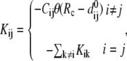
where 0 ≤ ≤1 is the anisotropy weight parameter (see below) and i or j is the index for a C_α atom. is the distance between the equilibrium positions of i and j. () is the three-dimensional (3D) displacement of i (j). is the unit vector pointing from the equilibrium position of i to that of j. is the force constant of the spring between i and j: = 10 C if i and j are bonded, and = C otherwise. C can be determined by fitting the crystallographic B-factors (see below). The use of two force constants for the bonded and nonbonded residue-residue interactions was shown to improve the performance of ENM (21) and GNM (12).

The physical basis for the weighted combination adopted in Eq. 1 is as follows. For a pair of contacting C_α atoms (i, j), can be partitioned into the longitudinal (parallel to ) and the transverse (perpendicular to ) components (see Fig. 1). In ENM, the stiffness for the latter component (the curvature of in Fig. 1) is zero, which leads to a fully isotropic (orientation-independent) interaction between i and j. In GNM, both components have the same positive stiffness (same curvature for and in Fig. 1), so the interaction between i and j is anisotropic (orientation-dependent). In G-ANM, gives the ratio of stiffness between the transverse displacement and the longitudinal displacement. Since = 0 corresponds to the isotropic limit, describes the extent of anisotropy in the contact interaction between i and j (thus named an anisotropy weight parameter).

FIGURE 1.

Physical basis of G-ANM potential function (see Eq. 1). The relative displacement between C_α atom j and i () is partitioned into longitudinal and transverse components that have different stiffness (see Methods for details).

The G-ANM potential energy is reformulated as follows:

(2)

where is the 3 N-dimensional displacement vector (N, number of residues or C_α atoms). is the ENM Hessian matrix. is the N by N Kirchhoff's matrix as defined in GNM, which is constructed as follows (9):

(3)

where is a 3 × 3 identity matrix, and is the Heaviside function.

At = 0, 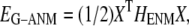and the G-ANM is reduced to an ENM. Note that the ENM potential is normally expanded in a quadratic form:

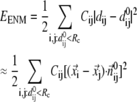( is the distance between C_α atom i and j at equilibrium).

At = 1, where 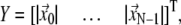and the G-ANM is reduced to a GNM (22).

Therefore G-ANM unifies GNM and ENM as its two limits.

For the Hessian matrix in Eq. 2, we perform the normal mode analysis, which yields 3 N-3 nonzero modes and 3 zero modes (corresponding to 3 translations) for and 3 N-6 nonzero modes and 6 zero modes (corresponding to 3 translations and 3 rotations) for (the ENM limit).

Evaluation of G-ANM in describing the crystallographic B-factors

By summing the nonzero modes of G-ANM, we compute the isotropic thermal fluctuations to simulate the isotropic crystallographic B-factor in a crystal structure as follows:

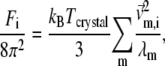(4)

where k_B is the Boltzmann constant, is the 3D component of the eigenvector of mode m at C_α atom i, is the eigenvalue of mode m, and T_crystal is the crystallographic temperature. The quality of G-ANM in fitting the B-factors is assessed by the cross-correlation coefficient 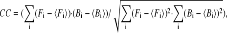where is the arithmetic average of over all C_α atoms.

For each test case, we compute the cross-correlation coefficient (CC) as a function of and (we only fit the B-factors of the first structure of the pair of structures in each test case). To remove sample heterogeneity, CC is normalized to 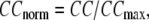where 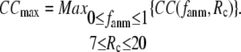Then the average () and standard deviation () are computed for among a selected list of 18 test cases (Table 1). A high quality of G-ANM in fitting B-factors is reflected by a high (low) value of ().

TABLE 1.

List of 22 pairs of protein structures from PDB

Protein	No. of residues	PDB codes and chains
Adenylate kinase	218	1aky, 2ak3A
Alcohol dehydrogenase	373	8adh, 6adhA
Annexin V	317	1avr, 1avhA
Calmodulin	144	1cll, 1ctr
Che Y protein	128	3chy, 1chn
Enolase	436	3enl, 7enl
HIV-1 protease	99	1hhp, 1ajxA
Lactoferrin	691	1lfh, 1lfg
LAO binding protein	238	2lao, 1lst
Maltodextrin binding protein	370	1omp, 1anf
Thymidylate synthase	264	3tms, 2tscA
Triglyceride lipase	265	3tgl, 4tgl
Tyrosine phosphatase	278	1yptA, 1lyts
Guanylate kinase	186	1ex7A, 1ex6A
Serum transferrin	328	1bp5A, 1a8e
Ras p21 protein catalytic domain	169	4q21, 5p21
Transducin-α	314	1tag, 1tndA
5-Enol-pyruvyl-3-phosphate synthase	427	1eps, 1g6sA
Oligo-peptide binding protein	517	1rkm, 2rkmA
RNA helicase	435	8ohm, 1cu1A
Myosin	730	1vom, 1mma
Rb69 DNA polymerase	897	1ih7A, 1ig9

Four pairs eliminated from the analysis are in bold (the selection removes those low-quality test cases if CC_max < 0.5 or CO_max < 0.5). The remaining 18 pairs are used for the evaluation of G-ANM.

Evaluation of G-ANM in describing the observed conformational changes

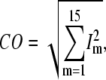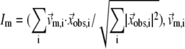The quality of G-ANM in describing the observed conformational changes is assessed by the cumulative overlap (CO) for the lowest 15 modes: where is the 3D component of the eigenvector of mode m at C_α atom i, and is the observed structural displacement at C_α atom i. We perform a similar normalization for and then compute the average () and standard deviation () of for the 18 selected test cases (Table 1). A high quality of G-ANM in describing the observed conformational changes is embodied by a high (low) value of ().

Comparison between the lowest modes of G-ANM and ENM

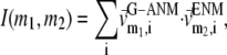We compute the cumulative similarity score between the lowest 15 modes of the G-ANM and that of the ENM: where and () is the 3D component of the eigenvector of mode () of the G-ANM (ENM) at C_α atom i. If the two sets of modes span the same subspace, SIM = 1; otherwise 0 ≤ SIM < 1. We note that as 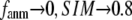instead of 1 because the lowest 3 nonzero modes of the G-ANM converge to the 3 rotational zero modes of the ENM. We compute the average () and standard deviation () of SIM for the 18 selected test cases as a function of and

RESULTS

We quantitatively assess the performance of G-ANM in describing both the isotropic thermal fluctuations and the observed conformational changes for a selected list of 18 test cases, each consisting of a pair of protein structures from the PDB. The list (Table 1) is compiled from an early work on ENM (17) and our recent work (23,24). We only include the crystal structures that do not have extensive interface between individual structural units.

Evaluation of G-ANM in describing the crystallographic B-factors

The quality of G-ANM in fitting the crystallographic B-factors is assessed by the CC between theoretical and experimental B-factors (see Methods). We analyze the average () and standard deviation () of “normalized” CC over a list of selected test cases (see Methods and Table 1).

and as a function of and are shown in Fig. 2, a and b. The -dependence of at fixed is as follows: for = 7 Å (8 Å), peaks at For ≥ 10 Å, the peak shifts to and its height decreases as increases. For 8 Å ≤ ≤ 20 Å, rapidly decreases as increases in 0 < < 0.1, and it becomes flat or slightly increases as increases in 0.1 ≤ ≤ 1. The observation that and vary substantially in 0 < ≤ 0.1 but change little in 0.1 ≤ <1 suggests that the introduction of small isotropic interactions (the first term of Eq .1) significantly improves the quality of G-ANM in fitting the B-factors to a level comparable with GNM. This improvement is much more pronounced for = 7 Å or 8 Å than for ≥ 10 Å: for = 8 Å, increases significantly from 0.64 at = 0 to 0.94 at and decreases sharply from 0.22 at = 0 to <0.05 at = 0.1.

FIGURE 2.

Average (a) and standard deviation (b) of the normalized cross-correlation coefficient between the experimental and theoretical B-factors. Average (c) and standard deviation (d) of the normalized cumulative overlap for the lowest 15 modes. Average (e) and standard deviation (f) of the cumulative similarity in the lowest 15 modes between the ENM and the G-ANM.

Then we examine the -dependence of at fixed for = 0 (the ENM limit), () is maximal (minimal) at = 20 Å and minimal (maximal) at = 7 Å, suggesting that the optimized fitting of the B-factors by ENM requires high (beyond the physical interaction range: 4.4 Å ∼ 12.8 Å, see Cieplak and Hoang (15)). However, the above -dependence is changed for 10⁻⁴ < < 0.1: the maximum (minimum) of () is moved to = 7 Å or 8 Å, which is now within the physical interaction range.

When and are both variable, the optimal fitting of the B-factors by GNM is attained at a physically realistic ∼8 Å and a small ∼ 0.1, instead of the ENM limit or the GNM limit.

Evaluation of G-ANM in describing the observed conformational changes

The quality of G-ANM in describing the crystallographically observed conformational changes is assessed by the cumulative overlap (CO) between the 15 lowest modes and the observed changes (see Methods). We analyze the average () and standard deviation () of “normalized” CO over a list of selected test cases (see Methods and Table 1).

and as a function of and are shown in Fig. 2, c and d. The -dependence of at fixed is as follows: for =7 Å (8 Å), is maximal at = 0.001 (0.003); for ≥ 12 Å, the maximum shifts toward higher and its height decreases gradually as increases. Similarly, for = 7 Å (8 Å), is minimal at = 0.001 (0.003); for ≥ 12 Å, the minimum shifts toward higher and its value increases gradually as increases. Notably, with the exception of = 7 Å, and change little in 0 < < 0.01, but vary substantially in 0.01 < ≤ 1. Therefore, small isotropic interactions (the first term of Eq .1) do not significantly degrade the quality of G-ANM in describing the observed protein conformational changes when compared with the ENM. Instead, for = 7 Å and 8 Å, an improvement in such quality is found.

Next we study the -dependence of at fixed for = 0 (the ENM limit), () is maximal (minimal) at = 8 Å and minimal (maximal) at = 20 Å, suggesting that the optimized description of the observed conformational changes by ENM requires a relatively small (contrary to the fitting of B-factors). With the exception of = 7 Å, the above -dependence is essentially maintained in 0 < ≤ 0.01, and the maximum (minimum) of () remains at = 8 Å.

When both and are variable, the optimal description of the observed protein conformational changes is achieved at a physically realistic = 8 Å and a small ∼ 0.003, which is slightly better than at the ENM limit.

Comparison between the lowest modes of G-ANM and ENM

To further understand the -dependence of the quality of G-ANM in describing the observed conformational changes, we will evaluate how much the lowest modes of the G-ANM differ from that of the ENM as varies using a cumulative similarity score SIM (see Methods).

The -dependence of at fixed resembles that of (Fig. 2 e): for = 7 Å and 8 Å, is peaked at = 0.001; for ≥ 10 Å, the peak disappears and the curve's right-side edge shifts toward higher as increases. For fixed () is lower (higher) at = 7 Å or 8 Å than at ≥ 10 Å. Thus, for < 0.01, the lowest modes of the G-ANM differ significantly from that of the ENM only if is relatively small ( ≤ 8 Å). Such difference is mainly due to the occurrence of extra zero modes in ENM for ≤ 8 Å (in addition to the 6 translational and rotational zero modes), which overestimate the mobility of the sparsely connected regions in ENM (such as a surface loop). The addition of the isotropic interaction energy (the first term of Eq. 1) in the G-ANM eliminates these additional zero modes in all the 22 test cases, thus removing a major source of errors in ENM.

DISCUSSIONS AND CONCLUSIONS

This work is, to our knowledge, the first attempt to unify GNM and ENM for the simultaneous modeling of both the thermal fluctuations and conformational motions in protein structures, despite recent efforts for model improvement within the framework of either GNM (12) or ENM (25). Our optimal solution is a generalized anisotropic network model parameterized with a physically realistic cutoff distance = 8 Å and a small anisotropy parameter ≤ 0.1. The optimal values of for describing thermal fluctuations and conformational motions are both small, although they are numerically different: the former (∼0.1) is higher than the latter (∼0.003). The contradicting parameter optimizations in ENM (the B-factors' fitting demands high whereas the description of observed conformational changes requires low ) are resolved in G-ANM: the optimal descriptions of both quantities are achieved at ∼ 8 Å.

The use of a relatively small is more advantageous because:

1. It agrees with the physical range of residue-residue contact interactions (including van der Waals and screened electrostatic interactions).

2. It enables more realistic modeling of medium-range (8–20 Å) interactions and couplings, which are crucial in allostery but obscured by large

3. Smaller also leads to lower computational cost in the normal mode analysis of ENM (or GNM), because the Hessian (or Kirchhoff) matrix is more sparse (note that the Hessian matrix of G-ANM is as sparse as that of ENM; thus the computational cost of the G-ANM is similar to that of ENM).

Due to the anisotropic geometry of amino acid side chains, the physical interactions between two contacting residues are intrinsically anisotropic: they depend on both the distance and the orientation between the two residues. The orientation-dependence, which is absent in the ENM potential, is incorporated in the G-ANM by introducing a new parameter > 0 that defines the extent of anisotropy between the longitudinal and transverse motions between pairs of contacting residues. Our result, in favor of a small suggests that the transverse motions are far less restrained energetically than the longitudinal motions, which may be explained by the high flexibility of side chains that facilitates easy accommodation to transverse motions between residues. This finding also validates the ENM as the zero order approximation to the G-ANM.

In our future studies, through proper parameterization of G-ANM (fitting the thermal fluctuations and/or the observed conformational changes with and ), we will strive to probe several key aspects of conformational dynamics in proteins such as the allosteric couplings (21,26) and the ligand-binding induced conformational motions (27). It will be interesting to assess the performance G-ANM in describing the anisotropic displacement parameters from crystallography (28) or structural fluctuations from NMR data (29). Comparison with other efforts to improve GNM (for example, see Song and Jernigan (30) and Erman (31)) also will be useful.

References

- 1.Tozzini, V. 2005. Coarse-grained models for proteins. Curr. Opin. Struct. Biol. 15:144–150. [DOI] [PubMed] [Google Scholar]
- 2.Ma, J. 2005. Usefulness and limitations of normal mode analysis in modeling dynamics of biomolecular complexes. Structure. 13:373–380. [DOI] [PubMed] [Google Scholar]
- 3.Bahar, I., and A. Rader. 2005. Coarse-grained normal mode analysis in structural biology. Curr. Opin. Struct. Biol. 15:586–592. [DOI] [PMC free article] [PubMed] [Google Scholar]
- 4.Tama, F., and C. L. Brooks. 2006. Symmetry, form, and shape: guiding principles for robustness in macromolecular machines. Annu. Rev. Biophys. Biomol. Struct. 35:115–133. [DOI] [PubMed] [Google Scholar]
- 5.Karplus, M., and J. A. McCammon. 2002. Molecular dynamics simulations of biomolecules. Nat. Struct. Biol. 9:646–652. [DOI] [PubMed] [Google Scholar]
- 6.Tirion, M. M. 1996. Large amplitude elastic motions in proteins from a single-parameter, atomic analysis. Phys. Rev. Lett. 77:1905–1908. [DOI] [PubMed] [Google Scholar]
- 7.Hinsen, K. 1998. Analysis of domain motions by approximate normal mode calculations. Proteins. 33:417–429. [DOI] [PubMed] [Google Scholar]
- 8.Atilgan, A. R., S. R. Durell, R. L. Jernigan, M. C. Demirel, O. Keskin, and I. Bahar. 2001. Anisotropy of fluctuation dynamics of proteins with an elastic network model. Biophys. J. 80:505–515. [DOI] [PMC free article] [PubMed] [Google Scholar]
- 9.Haliloglu, T., I. Bahar, and B. Erman. 1997. Gaussian dynamics of folded proteins. Phys. Rev. Lett. 79:3090–3093. [Google Scholar]
- 10.Bahar, I., A. R. Atilgan, and B. Erman. 1997. Direct evaluation of thermal fluctuations in proteins using a single parameter harmonic potential. Fold. Des. 2:173–181. [DOI] [PubMed] [Google Scholar]
- 11.Kundu, S., J. S. Melton, D. C. Sorensen, and G. N. Phillips Jr. 2002. Dynamics of proteins in crystals: comparison of experiment with simple models. Biophys. J. 83:723–732. [DOI] [PMC free article] [PubMed] [Google Scholar]
- 12.Kondrashov, D. A., Q. Cui, and G. N. Phillips Jr. 2006. Optimization and evaluation of a coarse-grained model of protein motion using X-ray crystal data. Biophys. J. 91:2760–2767. [DOI] [PMC free article] [PubMed] [Google Scholar]
- 13.Eyal, E., L. W. Yang, and I. Bahar. 2006. Anisotropic network model: systematic evaluation and a new web interface. Bioinformatics. 22:2619–2627. [DOI] [PubMed] [Google Scholar]
- 14.Yang, L. W., A. J. Rader, X. Liu, C. J. Jursa, S. C. Chen, H. A. Karimi, and I. Bahar. 2006. oGNM: online computation of structural dynamics using the Gaussian Network Model. Nucleic Acids Res. 34:W24–31. [DOI] [PMC free article] [PubMed] [Google Scholar]
- 15.Cieplak, M., and T. X. Hoang. 2003. Universality classes in folding times of proteins. Biophys. J. 84:475–488. [DOI] [PMC free article] [PubMed] [Google Scholar]
- 16.Cui, Q., and I. Bahar, editors. 2006. Normal mode analysis. In Theory and Applications to Biological and Chemical Systems. CRC press, Taylor & Francis Group, Boca Raton, FL.
- 17.Tama, F., and Y. H. Sanejouand. 2001. Conformational change of proteins arising from normal mode calculations. Protein Eng. 14:1–6. [DOI] [PubMed] [Google Scholar]
- 18.Delarue, M., and Y. H. Sanejouand. 2002. Simplified normal mode analysis of conformational transitions in DNA-dependent polymerases: the elastic network model. J. Mol. Biol. 320:1011–1024. [DOI] [PubMed] [Google Scholar]
- 19.Zheng, W., and S. Doniach. 2003. A comparative study of motor-protein motions by using a simple elastic-network model. Proc. Natl. Acad. Sci. USA. 100:13253–13258. [DOI] [PMC free article] [PubMed] [Google Scholar]
- 20.Nicolay, S., and Y. H. Sanejouand. 2006. Functional modes of proteins are among the most robust. Phys. Rev. Lett. 96:78104–78107. [DOI] [PubMed] [Google Scholar]
- 21.Ming, D., and M. E. Wall. 2005. Allostery in a coarse-grained model of protein dynamics. Phys. Rev. Lett. 95:198103. [DOI] [PubMed] [Google Scholar]
- 22.Chennubhotla, C., A. J. Rader, L. W. Yang, and I. Bahar. 2005. Elastic network models for understanding biomolecular machinery: from enzymes to supramolecular assemblies. Phys. Biol. 2:S173–S180. [DOI] [PubMed] [Google Scholar]
- 23.Zheng, W., and B. R. Brooks. 2005. Normal modes based prediction of protein conformational changes guided by distance constraints. Biophys. J. 88:3109–3117. [DOI] [PMC free article] [PubMed] [Google Scholar]
- 24.Zheng, W., and B. R. Brooks. 2006. Modeling protein conformational changes by iterative fitting of distance constraints using re-oriented normal modes. Biophys. J. 90:4327–4336. [DOI] [PMC free article] [PubMed] [Google Scholar]
- 25.Song, G., and R. L. Jernigan. 2006. An enhanced elastic network model to represent the motions of domain-swapped proteins. Proteins. 63:197–209. [DOI] [PubMed] [Google Scholar]
- 26.Zheng, W., and B. R. Brooks. 2005. Identification of dynamical correlations within the myosin motor domain by the normal mode analysis of an elastic network model. J. Mol. Biol. 346:745–759. [DOI] [PubMed] [Google Scholar]
- 27.Zheng, W., and B. R. Brooks. 2005. Probing the local dynamics of nucleotide-binding pocket coupled to the global dynamics: myosin versus kinesin. Biophys. J. 89:167–178. [DOI] [PMC free article] [PubMed] [Google Scholar]
- 28.Kondrashov, D. A., A. W. Van Wynsberghe, R. M. Bannen, Q. Cui, and G. N. Phillips, Jr. 2007. Protein structural variation in computational models and crystallographic data. Structure. 15:169–177. [DOI] [PMC free article] [PubMed] [Google Scholar]
- 29.Yang, L. W., E. Eyal, C. Chennubhotla, J. Jee, A. M. Gronenborn, and I. Bahar. 2007. Insights into equilibrium dynamics of proteins from comparison of NMR and X-ray data with computational predictions. Structure. 15:741–749. [DOI] [PMC free article] [PubMed] [Google Scholar]
- 30.Song, G., and R. L. Jernigan. 2007. vGNM: a better model for understanding the dynamics of proteins in crystals. J. Mol. Biol. 369:880–893. [DOI] [PMC free article] [PubMed] [Google Scholar]
- 31.Erman, B. 2006. The Gaussian network model: precise prediction of residue fluctuations and application to binding problems. Biophys. J. 91:3589–3599. [DOI] [PMC free article] [PubMed] [Google Scholar]