Structural and dynamic properties of water around acetylcholinesterase

Abstract

Structural and dynamic properties of water molecules around acetylcholinesterase are examined from a 10-nsec molecular dynamics simulation to help understand how the protein alters water properties. Water structure is broken down into hydration sites constructed from the water density <3.6 Å from the protein surface. These sites are characterized according to occupancy, number of water neighbors, hydrogen bonds, dipole moment, and residence time. The site description provides a convenient means to describe the extent and localization of these properties. Determining the network of paths that waters follow from site to site and measuring the rate of flow of waters from the sites to the bulk make it possible to quantitatively study the time scales and paths that water molecules follow as they move around the protein.

The relationship between water and proteins has been a well-researched topic over the past few decades. Much has been learned about the unusual properties relative to bulk that water exhibits due to the presence of the protein, particularly in the first hydration shell (Rupley and Careri 1991; Teeter 1991; Levitt and Park 1993; Karplus and Faerman 1994; Pettitt et al. 1998). However, much remains to be discovered concerning how these properties relate to protein structure and protein function.

To date, most knowledge of water properties around proteins has come from experimentation. In particular, high-resolution X-ray and neutron diffraction methods are able to reveal water positions, their extent of disorder, orientation in the case of neutron diffraction, and occupancy (Savage and Wlodawer 1986; Schoenborn et al. 1995; Carugo and Bordo 1999). NMR methods provide not only structural, but also dynamic information such as the residence times of waters in certain locations (Otting et al. 1991; Denisov and Halle 1996; Wiesner et al. 1999) and find water residence times in and around proteins ranging from 10⁻²–10⁻⁹ sec. Femtosecond fluorescence (Pal et al. 2002) shows surface waters moving at two time scales, 1 and 40 psec, corresponding to a bulk-like local motion and a local residence time, respectively. Recently, computer simulations have proven to be an increasingly powerful tool in modeling the behavior of water around proteins (Wong and McCammon 1986; Brooks and Karplus 1989; Brunne et al. 1993; Roux et al. 1996; Zhang and Hermans 1996; Helms and Wade 1998; García and Hummer 2000; Luise et al. 2000; Makarov et al. 2000). Although still limited to system sizes of a single protein and time scales on the order of nanoseconds, the greatest strength of computer simulation is its ability to track individual water molecules around proteins, something currently beyond the capability of experiment.

This work seeks to examine in detail the properties of water around the enzyme, acetylcholinesterase (AChE), from a recently reported 10-nsec molecular dynamics simulation (Tai et al. 2001) to provide insight into how water may affect protein properties such as ligand binding. This simulation provided an opportunity to examine water properties around a large protein and over a long simulation time scale. It builds on a previous study of water in the active site gorge of AChE (Henchman et al. 2002). Raw molecular dynamics simulations contain trajectories of thousands of waters. Their properties will change according to where they lie relative to the protein. What is more useful is to describe water properties at a given point in space. Therefore, this trajectory data is reduced to the more interpretable form of hydration sites (Lounnas and Pettitt 1994) in the spirit of hydration sites seen in X-ray crystal structures. This permits a powerful and precise description of the spatial variation of water properties around the protein. The ARC/TAP (averaged residue coordinate/time-average position) hydration site method (Henchman and McCammon 2002) is used to construct hydration sites from the water density by use of coordinate system local to each hydration site. The properties of each water are then assigned to the nearest site. The extent of each property is quantified by summing over all hydration sites. Properties studied include site occupancy, number of neighboring waters, hydrogen bonds, and average dipole moments. In addition, a large range of dynamic properties are studied. These are residence time, intersite jump times, surface water flux between the protein surface and bulk, and TAP (time-averaged position) for the whole system.

Results

The properties of hydration sites in most cases are represented in two ways. The first method uses graphical color-coded plots so that the spatial variation of properties may be visualized. The second method uses property histograms over all of the sites, so that the importance of the value of a given property may be quantitatively assessed.

Water density and hydration sites

The water density around AChE is illustrated in Figure 1 ▶. As discussed in earlier work (Henchman and McCammon 2002), the density produced by the ARC/TAP method takes into account noise from water and protein motion. This leads to a cleaner, sharper density from which hydration sites may be better resolved. The protein appears to be covered fairly uniformly with distinct localized regions of higher density representing the hydration sites. There is a wide distribution in the sizes of these regions. In general, the larger the region, the more concentrated and well defined the density. Regions closer to the protein are more ordered, whereas those regions further away and closer to more mobile parts of the protein, such as the chain termini, are more disordered. From this density, 1476 sites are obtained altogether within 3.6 Å of any protein atom. These are illustrated in Figures 2 and 4 ▶ ▶ below, the same sites in the same orientation each time, colored according to a different property. A comparison of site positions with x-ray sites of mAChE (Tai et al. 2002) has been reported previously (Henchman and McCammon 2002) and showed that of the 189 sites resolved in the crystal structure, there was a simulation site within 1.2 Å on average.

Fig. 1.

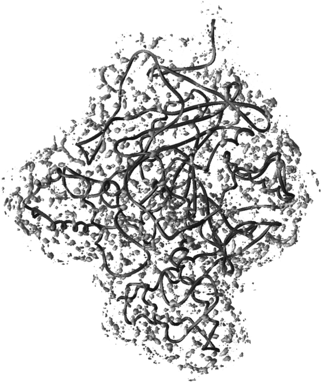
Water density isocontour for ρ_cut = 7× the bulk water density. AChE is the dark gray ribbon, oriented with the amino terminus at the top and carboxyl terminus at the lower left. In the middle is the active site gorge.

Fig. 2.

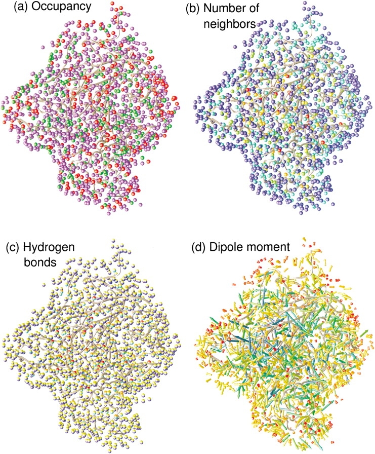
Structural water properties of the sites around AChE. AChE is the dark gray ribbon. (a) (Occupancy) Green sites have occupancy <0.75, red >1.25, and blue in between. (b) Number of neighboring waters; red, orange, yellow, green, cyan, and blue are 0, 1, 2, 3, 4, and 5 or more, respectively. (c) Number of hydrogen bonds; yellow, orange, and red hemispheres indicate 0, 1, or 2 water-residue hydrogen bonds, and green, aqua, cyan, and blue hemispheres indicate 0, 1, 2, or 3 water–water hydrogen bonds. (d) Dipole moment; red, orange, yellow, green, cyan, and blue are <0.2, centered on 0.7, 1.2, 1.6, 2.1, and >2.3 D, respectively.

Fig. 4.

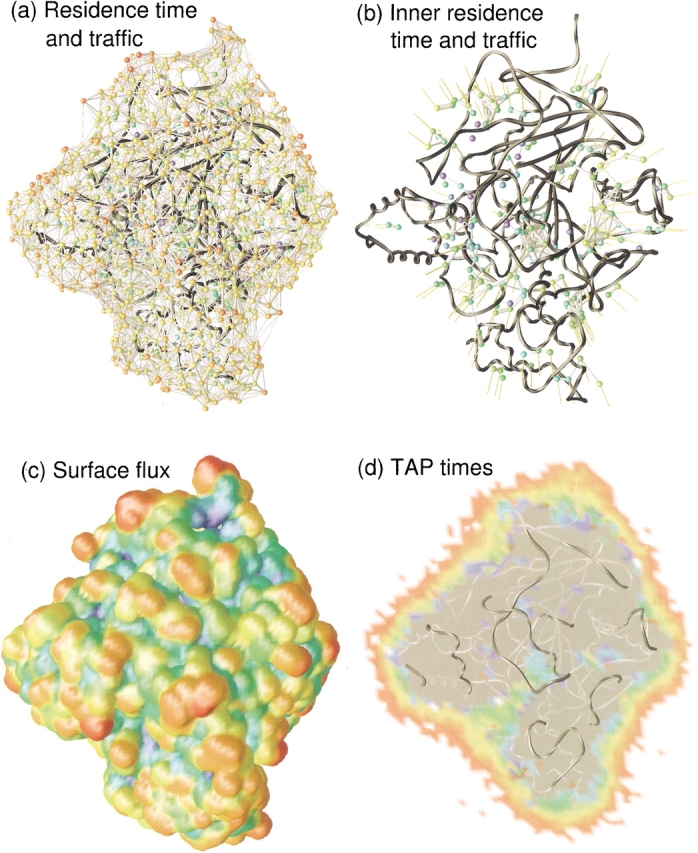
Dynamic water properties of the sites around AChE. AChE is the dark gray ribbon. (a) Water residence time and intersite traffic; red, orange, yellow, green, cyan, and blue are 10, 50, 100, 500, 2000, and 10,000 psec residence times; bar thickness scales exponentially with number of traffic events from 5 to 80 or more. (b) Water residence time and intersite traffic for a subset of sites in the protein interior as described in the text. Residence time coloring is the same as in a, whereas traffic events now scale exponentially from 1 to more than 16. The yellow lines indicate connections to the bulk. (c) Surface flux of waters between all sites and the bulk projected onto the solvent accessible surface of AChE. Blue, green, yellow, and red are 100, 300, 700, and >1000 transits, respectively. (d) Cross-section of TAP times in the whole box. White is <20 psec, red is 20 psec, green 100 psec, and dark blue at 10 nsec. The area shaded gray is the protein cross-section.

Occupancy

The sites in Figure 2a ▶ are colored according to their occupancy and the distribution of occupancy appears in Figure 3a ▶. The average occupancy for all sites is 1.01. This single occupancy is a consequence of the values chosen for the ρ_cut and r_cut parameters used to create sites as described in the Materials and Methods section. The majority of sites, 925, colored blue, are singly occupied. However, 279 sites, colored red, have occupancy >1.25 and 272 sites, colored green, have occupancy <0.75. These deviations arise for a number of reasons. First, the hydration site description of water is only an approximation to its structure. Whereas waters more often than not occupy hydration sites, they are still somewhat disordered and may often lie on the boundary between sites. Second, although sites are designed to follow the protein, protein motions may still alter site positions to some extent. Third, some sites, particularly those surrounded by a lot of protein, may truly become empty at times. Fourth, the extreme sites at each end of the histogram come predominantly from the sites most in the bulk, where there are edge effects and less well-defined sites. Overall, the figure shows that use of hydration sites is a reasonable but not exact method of describing water structure.

Fig. 3.

Histograms of site properties illustrated in Figs. 2 and 4 ▶ ▶. These are (a) site occupancy, (b) number of neighboring waters, (c) number of water-residue hydrogen bonds, (d) number of water–water hydrogen bonds, (e) average magnitude of dipole moment, (f) τ with line of best fit, (g) τ_jump for all jumps, those that happen at least five times, and nonbulk jumps, and (h) surface water flux between sites and the bulk.

Number of neighbors

The extent of solvent exposure for each site is measured by the average number of neighboring waters within the cutoff distance, 3.6 Å, of all waters that reside in the site, as seen in Figures 2b and 3b ▶ ▶. As would be expected, sites on the surface, colored blue, are the most solvent exposed with five or more neighbors, whereas red sites in the interior have no neighbors. A total of 839 sites are essentially bulk-like with 5 neighbors. At the other end, 20 sites appear to be completely isolated in the protein, whereas 31 have ∼1 neighbor. Such a large number of buried waters in the protein, almost double that of the average protein, has been noted previously from the AChE crystal structure of another species, Torpedo californica (Koellner et al. 2000). It is unknown whether this serves some functional role or merely reflects the nature of the AChE fold.

Hydrogen bonds

The average number of hydrogen bonds for each site conveys similar information to the number of neighbors and accords fairly closely with intuition. Figure 2c ▶ colors each site according to water–water and water–protein hydrogen bonds, whereas Figure 3, c and d ▶ show their distribution. Broadly speaking, there are three types of water (see caption for color coding) as follows: the blue-yellow bulk-like waters with only water–water hydrogen bonds, which are more distant from the protein surface, the green-red waters with only water–protein hydrogen bonds buried in the protein, and the waters at various stages in between. Only 274 sites have one or more hydrogen bonds with the protein. Although there is variation in the types of hydrogen bond, most sites have a similar number of total hydrogen bonds. The average number of hydrogen bonds over all sites is 3.8, indicating that the total number of hydrogen bonds is not so useful as a measure to account for the range of site properties.

Dipole moment

The average dipole moment is shown in Figures 2d and 3e ▶ ▶. The color and length of the arrow both indicate the size of the average dipole moment. Blue is largest and red smallest. The more ordered the waters in the site, the closer the average value to the instantaneous value (2.39 D for SPC/E), whereas the more disordered the water, the smaller the average dipole moment due to cancellation. These results also conform with intuition. Typically, buried waters have the most ordered blue dipoles, bulk-like waters on the surface have negligible average dipole moment (<0.2), whereas the remaining waters lie in between with varying degrees of order. These data also illustrate the extent of orientational ordering. On average, there is a trend for dipoles to point inward toward the negatively charged AChE (charge is −10). This effect may be roughly quantified by taking the dot product of the dipole moment with a unit vector from the AChE center of mass to the site. The average value of this quantity over all sites is −0.16 D, indicating the tendency for dipoles to point inward. Some regions appear to have local ordering, but close to the protein, dipoles point in many directions as they are influenced most strongly by the details of the protein surface.

Residence times

Residence times correspond to the time that a water spends in a site before moving to another site. Figure 4a ▶ colors the sites by residence time. The sites with the longest residence times are the blue buried sites. It is much harder for waters trapped in the protein to escape the confinement. A total of 20 sites have residence times of 10 nsec, the full simulation time. Presumably, their real residence times are potentially orders of magnitude longer and outside of the time scale of the simulation. At the other end of the time scale, waters on the surface colored in red have residence times <10 psec. The longest-lived waters on the surface and exposed to bulk water are the yellow waters with residence times ∼100 psec. Longer residence times are found in cavities such as the active site gorge (Henchman et al. 2002) and other crevices on the surface. Figure 4b ▶ shows a clearer picture of the buried sites, selected as those that exchange less than five times with the bulk. A few sites have residence times ∼100 psec but the majority are >500 psec. A log–log plot of the distribution of τ shown in Figure 3f ▶ is found to be roughly linear, as seen for the residence time distribution found in another work around cytochrome c (García and Hummer 2000). The spike at 10⁴ psec includes all waters with τ >10⁴ psec. Fitting to the linear section in the middle, the power-law scaling exponent is −0.84. However, this is quite different to the exponent of −2.5 found for cytochrome c, a protein a fifth the size of AChE. Variations in the τ calculation for each work might account for some of the difference but the distribution of τ is probably quite dependent on protein size and likely to be unique for each protein.

A number of studies have been done on what properties determine residence times. The general conclusion appears to be that the clearest factor is the topology of the protein surface (Luise et al. 2000; Makarov et al. 2000). Although the nature of the amino acids may play a secondary role, studies on the nature of the amino acids adjacent to hydration sites have not been conclusive (Brunne et al. 1993; García and Stiller 1993; Muegge and Knapp 1995; Abseher et al. 1996). The lack of a simple relationship between residence time and amino acid arises for a number of reasons. First, the amino acid distribution in proteins is not uniform, with more hydrophobic residues buried in the protein. Even though waters form stronger interactions with polar residues, because these residues have a greater tendency to lie on the surface, water residence times near them will actually be shorter, whereas those near buried hydrophobic residues may be longer. Second, the same site typically lies next to multiple types of amino acid. Residence time would depend collectively on all of these amino acids in a manner that would make it difficult to attribute a relationship to each individual amino acid. Third, amino acids can possess conflicting attributes relating to residence time. For example, they may be highly charged, which favors stronger interactions and longer τ but are also more mobile, lowering τ. The results from this work support the idea that the protein topology is the main factor affecting residence time. The measure used to study this hypothesis in this work is the average number of water neighbors within 3.6 Å of all waters while they were in the site. The less water neighbors a site has, the more buried it is in the protein. Residence time, τ versus number of neighbors is shown in Figure 5 ▶. The relationship is quite clear with a correlation coefficient of 0.90, although other factors do come into play. For example, a water in the active site gorge, for example, has many neighbors, yet is overall fairly confined. τ would depend in a complex way not only on the number of neighbors, but also iteratively on their neighbors’ τs.

Fig. 5.

Plot of residence time, τ, versus number of water neighbors (solid) with line of best fit (dashed).

Intersite traffic

As well as knowing the duration of waters in sites, it is interesting to understand how they move around. In a computer simulation, it is straightforward to follow the progression of each water molecule. By use of the site representation of water, water motions may be discretized into jumps between sites. The information of most interest is not the trajectories of individual water molecules, but the flow of water between sites. Once a water moves to a new site, it generally loses memory of its previous trajectory. The number of waters moving either way between two sites is referred to as the intersite traffic. At equilibrium assuming single occupancy for each site, there is no preferred direction and the rate forward equals the reverse rate. In a finite length simulation there is invariably noise and this equality is close but not exactly true. A plot of forward traffic versus reverse traffic (data not shown) has a line of best fit with slope 1.00 and a correlation coefficient of 0.996 supporting this. This traffic is illustrated in Figure 4a ▶ by the bars connecting the sites. The thicker the bar, the more waters that pass between the sites. The thinnest bars represent five transits, whereas the thickest bars represent >80 transits. Traffic out into the bulk is omitted for clarity. On the surface, sites appear to exchange with all of their neighbors, some more than others. The largest amount of traffic is parallel to the surface as expected, as both sites have low residence times and will exchange the most frequently.

A clearer view of the traffic inside the protein may be seen in Figure 4b ▶, which shows sites that exchange with the bulk less than five times. In this case, the thinnest bars correspond to 1 transit and the thickest to >16. The yellow bars are drawn from sites that exchange with the neighboring sites closer to the surface that are not shown. There are few waters that do not move at all, some site pairs with a rather high exchange rate between them, and clusters of a range of sizes that connect to the surface. The active site gorge is the cluster of waters at the center of the protein. It connects with the bulk on a line partly running left, down, and out of the page. The water sites in the active site gorge are described in detail elsewhere (Henchman et al. 2002). Another cluster of water is seen on the right. This lies outside of the so-called backdoor, an alternative passage that is suspected to lead into the active site gorge (Gilson et al. 1994; Tai et al. 2001). A number of pockets are seen elsewhere on the surface of AChE. Inside the protein, some other small single-file passages are seen, along which only one or two waters move during the 10 nsec, showing that some buried waters are able to move around slowly inside the protein. However, the traffic information inside the protein involving only a few jumps should be treated with caution, because in general, the time scales for their motion are long and poorly sampled by this simulation, and waters here may not even be equilibrated.

Some statistics about jumps also give some insight. In the whole simulation, 738,430 jumps were recorded in total involving at least one site. A total of 61% of these are between a site and the bulk, whereas the remainder are jumps between sites. A total of 6% of jumps land a water in the same site that it started. These waters probably get slowly forced out of their site only to drop back in again. When a water jumps to a new site, usually another water will move in to replace it. Only 0.1% of jumps involve the direct exchange of waters between two sites, in which the maximum difference in time allowed for the second water to replace the first is 3 psec. Such an occurrence near the protein is a rare event, as waters must push past each other. Jumps involving the bulk or greater than two sites are much more common. Direct exchange between a site and the bulk makes up 11% of jumps, but it is not clear whether the water moving into the bulk directly replaces the one that entered. The majority of jumps appear to be much more concerted, involving three waters or more, and typically have at least one exchange with the bulk. For example, for 33% of intersite jumps, at least one of the waters that is replacing or vacating either site exchanges with the bulk within 3 psec of the other water moving. Many of the other intersite jumps are part of a larger network of almost simultaneous jumps involving at least one bulk water. As well as looking at the statistics for the total number of jumps, jumps may be accumulated into jump types, defined between a given pair of sites or the bulk. There are 17,814 unique types of jump type, with 56% (9976) of these occurring five times or more. Considering only these significant jump types, this gives each site on average ∼12 types of jump (1476 sites). Most of these significant jump types, 8641, are between two sites, represented by a bar in Figure 4a ▶. The difference, 1335 jump types, are exchanges between a site and bulk. Thus, 1476 − 1335 = 141 sites that do not exchange directly with the bulk. All of these sites, shown in Figure 4b ▶, lie inside the protein.

Jump times

Jump times, τ_jump, may also be calculated analogously to residence times by fitting to a survival function defined by equation 1. The distribution of jump times is illustrated in Figure 3g ▶. Jump times span three orders of magnitude, just as for residence times. However, the shape of the distribution is quite different from that for residence times. It appears at first surprising that the most common type of jump events have the longest τ_jump. Considering only significant jump types (those happen at least five times), it may be seen in Figure 3g ▶ that a large number of jump types account for the jumps with τ_jump ∼ 10³ − 10⁴ psec. This behavior may be better understood by examining the relationship between τ_jump and the distance of the jump. Figure 6 ▶ qualitatively suggests how τ_jump changes with distance. Jumps of 2–4 Å span the whole time scale and most commonly are ∼10³ psec, whereas longer jumps at 6–8 and 8–10 Å are more on the ∼10⁴ psec time scale with very few below 10³ psec. This distribution of jump times is now fairly intuitive. A water has a greater choice of sites to move to the further away they are, but the longer the jump, the less likely it is to occur, because closer jumps are easier to make and occur more often. At the other end of the time scale are jumps between sites and the bulk. Figure 3g ▶ also shows the distribution of all jump times, τ_jump, not involving bulk sites. From this, it can be seen that most jumps involving the bulk are on the 10¹–10² psec time scale, and that the fastest jumps on the protein surface between sites are ∼30 psec.

Fig. 6.

Histogram of the distribution of jump rates, τ_jump, for jump distances within a given range, 2–4, 4–6, 6–8, and 8–10 Å.

Individual jump times provide another means to calculate residence times. By use of equation 2, the sum of all of the out rates (inverse of jump times) to all neighboring sites gives the rate at which a water leaves the site, the inverse of which is the residence time. Residence times are calculated from both in and out rates and averaged to give a final residence time, τ_Σjump. A plot of residence time by this method versus residence time calculated from TAP times is given in Figure 7 ▶. The slope of the line of best fit passing through the origin is 0.98 and the correlation coefficient is 0.89. Both definitions of τ give similar results, but there is still some discrepancy, particularly for large τs. The distribution of τ_Σjump is very similar to that of τ in Figure 3f ▶ (data not shown). The only significant difference is for those sites with τ = 10 nsec. τ_jump cannot be measured if the water never moves from the site. Viewed in this way, residence times are seen to depend not simply on some local property of the site, but rather on the distribution of τ_jump leading to the site. In other words, the residence time depends collectively on the free energy barriers leading out of the site. To rationalize residence times, the question then turns to what these τ_jump depend on. Only qualitative relationships could be observed that influence τ_jump. The further apart the sites, or the more buried one or both of the sites, the larger the τ_jump. Each τ_jump is likely to depend both on the shape of the passage connecting two sites and how easily the water in the destination site can move elsewhere. Such processes cannot be quantified easily without an exquisitely detailed analysis.

Fig. 7.

Residence times, τ_Σjump, calculated from jump times versus τ from TAPs.

Surface water flux

The flux between the hydration sites on the protein surface and the bulk is shown in Figures 3h and 4c ▶ ▶. The number of transits between each site and the bulk is calculated and this value is assigned to a 0.5 Å grid. This grid is then projected onto the solvent-accessible surface of AChE. The redder regions have the highest flux of >1000 transits in the 10 nsec (0.1 ps⁻¹), whereas blue regions have <100 (0.01 ps⁻¹). Surface flux appears to be almost entirely a function of surface topology. The prominent convex regions of the protein have the highest flux, whereas the concave crevices have the lowest. This information is consistent with residence times and their dependence on the number of neighboring waters described earlier. No special properties may be seen near the entrance to the active site gorge lying immediately to the left of the central red prominence that may assist in the function of the enzyme.

Bulk TAP times

Further away from the protein, water is less structured, and the concept of a hydration site is undefined. Hence, a more convenient measure of water mobility is TAP times calculated in the protein frame. The diffusion coefficient is another possible measure, but its anisotropic nature and the discrete size of water make it problematic to measure as a spatially dependent property. Figure 4d ▶ shows a two-dimensional cross-section of TAP time through the middle of the protein. The longest TAP times of ∼10 nsec are blue and generally lie buried in the protein. TAP times of 20 psec are red and on the surface. Significant perturbations from the bulk occur out to 5–10 Å from the protein surface (to set the scale, the widest width of the protein as seen in Figure 4d ▶ is 70 Å) in agreement with earlier work on diffusion coefficients (Wong and McCammon 1986). Longer TAPs than average occur in the concave regions. The gorge is clearly visible on the lower left cutting through the protein cross-section. TAP times progressively increase, moving down through the gorge into the active site. TAP times in the bulk are around 10 psec on average, but these cannot be clearly resolved due to simulation noise, as is already evident from some of the scattered red specks. Hence, it is not possible to deduce whether slowing of waters occurs at distances greater than 10 Å. Such regions with TAP times below 10 psec are colored white. When projecting information onto a grid, a balance must be struck between using a large grid size to sample many waters to get good statistics on one hand, and having a fine enough grid to show detail on the other. A 1.5 Å grid was chosen for this figure as a suitable compromise. The better statistics reported earlier when using hydration sites to describe water properties illustrates one of the benefits of a site-based representation of water with a few thousand points versus a grid-based method with hundreds of thousands of points.

Discussion

A 10-nsec computer simulation of a large solvated protein has been used to examine how the protein affects water properties. The ARC/TAP hydration site method (Henchman and McCammon 2002) has been used to characterize water structure. This method resolves hydration sites from the water density by removing noise of random water motion and allowing for protein flexibility (Henchman and McCammon 2002). A hydration site description of water provides a precise and convenient means to describe the variation of water properties in space, to quantify the extent of the properties, and to describe how water molecules move around the protein.

This study of water around AChE has revealed the diverse properties of water molecules according to which site they occupy around the protein. The number of neighboring waters for a site decreases the more buried the site is inside the protein. This quantity provides a convenient measure of how buried all of the waters are. At the extreme end, altogether 20 sites lie essentially isolated from all other water in the protein, whereas at the other end, 839 sites are essentially bulk like with 5 water neighbors. For hydrogen bonds, few of the sites surrounding the protein actually have hydrogen bonds with protein atoms, with only 274 sites having 1 or more. The more buried they are, the larger the number of water-residue hydrogen bonds. On the other hand, waters closest to the bulk have the most water-water hydrogen bonds. On average, these effects complement each other and most waters have a total number of hydrogen bonds close to the average of 3.8. Average site dipole moments are the largest and most ordered inside the protein, because the protein holds the waters there in place. Moving toward the bulk, their magnitudes become increasingly smaller and their directions disordered, tending toward zero dipole moment, characteristic of bulk water.

Much of the focus of this work is on the dynamic nature of water molecules. A wide range of residence times has been detected ranging from 10¹–10⁴ psec. No doubt longer and shorter τs exist. Longer τs are not detected by a 10-nsec simulation. Shorter τs will not be detected with the 3-psec positional averaging used to determine whether a water has left the site. This averaging prevents transient perturbations in water position terminating a TAP, even though the water almost immediately returns to the site. The use of ARC coordinates further ensures that what is being measured is how long a water stays near a group of residues, not how long it stays near a certain point relative to the whole protein. The value of τ increases exponentially the more buried the site is, as shown by a strong relationship between log τ and number of neighbors. Values of τ for sites close to bulk are ∼10 psec. The number of sites with a given residence time scales as a power-law with exponent −0.84. A total of 20 waters have the maximum measurable τ = 10 nsec, the full simulation time. These are not exactly the same 20 waters that are buried completely in the protein—only 12 waters share both properties. Nevertheless, all mostly buried waters have at most one or two neighbors. Residence times, τ_Σjump, are also calculated from jump times to and from the site. τ_Σjump is found to agree well with τ from TAP times.

The amount and rate of water traffic between sites is also examined. Most traffic involves exchanging with the bulk. Most exchanges with the bulk occur at the most exposed regions of the protein surface with frequencies as high as 0.1 ps⁻¹. The fewest exchanges are from sites in the protein crevices with frequencies around 0.01 ps⁻¹. The next most common type of jump event is across the surface of the protein, although many exchange events occurring on the surface are coupled to a second exchange with the bulk. Few jumps involve the direct exchange of waters between two sites; more commonly, they involve the concerted jumping of three or more waters. The rate of site to site exchange is reduced either when at least one site is significantly buried or the sites are widely separated. Inside the protein, jump events are the least frequent of all. Only a few infrequently occurring single-file water paths are visible inside the protein.

Hydration sites, although an approximation, have proven to be a convenient means to describe water structure, properties, and dynamics. Understanding the nature of water behavior around a protein can give useful insight into how proteins influence their environment and interact with other molecules. It is important to bear in mind that the numbers quantifying these properties have come from a computer simulation and are only approximate. However, the large number of waters passing through most sites leads to more reliable statistics for the properties of these sites. The longest-lived waters would have the least accurate data. Currently, good statistics for the dynamics of molecules interacting with proteins using fully atomistic simulations may be obtained only for water molecules, but the results are helpful in assessing how larger molecules and ions might be affected. Whereas the properties measured are specific to acetylcholinesterase, they would be expected to be qualitatively similar for other proteins in general. Knowledge of water behavior around proteins is also useful for designing more realistic reduced representation models of solvent that account for the variation in water behavior, which usually assume identical behavior for all water molecules. In summary, this work supports the now well-established view that proteins should not be thought of as simply a single molecule, but as a more expansive, hydrated complex.

Materials and methods

Simulation protocol

Full details of how the system is set up are given in a previously reported 1-nsec simulation (Tara et al. 1999). In summary, the system consists of mouse AChE (Bourne et al. 1995) (Protein Data Bank identification code: 1MAH) in a box of 25205 SPC/E waters and 10 sodium ions added to maintain system neutrality. For the water setup in particular, there were no crystal water molecules in the 1MAH structure. Therefore, waters were placed inside the protein by use of the GRID program (Goodford, 1985). The criteria for water placement in a cavity was that the water’s energy be less than −46 kJ mole⁻¹ and that it make at least two hydrogen bonds. The protein was then solvated in a cubic box (edge 96 Å) of pre-equilibrated waters. Waters closer than 2.6 Å to any protein heavy atom were removed. Nine sodium ions were placed in the solvent at ∼5 Å from the protein surface, and one sodium ion was placed in the choline-binding pocket of the active site gorge. The full 10-nsec equilibrated MD trajectory used in this analysis has been reported previously (Tai et al. 2001). The simulation was run on a Cray T3E using the NWChem program (Straatsma et al. 2000), the AMBER 94 force field (Cornell et al. 1995), particle mesh Ewald summation (Darden et al. 1993), SHAKE (Ryckaert et al. 1977) for bonds involving hydrogens, and constant temperature and pressure reservoirs (Berendsen et al. 1984), set to 298.15 K and 1 atmosphere, respectively. Snapshots for analysis were saved every 1 psec.

Water analysis

The water density is built up from the water oxygen positions in all 10,000 simulation frames by use of the recently described ARC/TAP method (Henchman and McCammon 2002). Unless otherwise mentioned, properties of waters are based on the position of their oxygen atom. First, the TAP of each water within 3.6 Å of any protein atom is calculated in the reference frame of each neighboring residue. At a later time, the TAP of the water may be calculated in the protein frame as the average position with respect to each neighboring residue weighted by the number of times that this residue was a neighbor of the water. The TAP is updated continually as long as the water’s position averaged over the three previous frames remains within 2.8 Å of the TAP. This averaging provides a more robust check of whether the water has left the TAP. When a water leaves a TAP, it forms a new TAP. Second, the water density is constructed from all of the TAPs on a 0.5 Å grid covering the entire protein by projecting the TAPs in ARC onto a single protein frame. The first frame of the 10 nsec is chosen for this construction. Each TAP is placed on the grid with value given by the lifetime of the TAP. Third, hydration sites are extracted from the water density in the following manner. All maxima with ρ > ρ_cut = 7 × the average water density become sites, and any sites closer than r_cut = 2 Å to each other are merged iteratively on a nearest-neighbor basis to give the final site definitions. As noted earlier (Henchman and McCammon 2002), the number of sites does depend on the choice of these two parameters, ρ_cut and r_cut. The parameters used here were chosen to produce sites whose average occupancy is one. All TAPs are then placed in the closest site within 2.8 Å, a slightly larger distance than the TAP spacing to ensure that all nearby TAPs are placed in one site. Because the density is only built from waters in TAPs that approach closer than 3.6 Å to the protein, almost all hydration sites found are also within 3.6 Å from the protein. The few sites that are more distant than 3.6 Å are removed.

Site properties are divided into two broad categories—structural and dynamic. The structural properties are number of water neighbors, occupancy, number of hydrogen bonds, and dipole moments. These properties are calculated as the average property of each contributing TAP weighted by the lifetime of that TAP. Four dynamic properties are considered as follows: residence times, intersite jump times, protein surface water flux, and bulk TAP times. The residence time is calculated by two methods. The first is from the site survival function, S(t), (Impey et al. 1983) given by

(1)

S(t) gives the fraction of total waters, N_water, that remain in a site after a given time, t. P_i(t) is a binary function that equals one if water i is still in the site after time t, and zero otherwise. A single exponential fit to S(t) ∝ exp(−t/τ) yields a residence time, τ, for that site. It is helpful to note that τs are generally longer than average TAP times. The second method for calculating residence time is from the intersite jump time. The intersite jump time is calculated in an analogous way to the residence time from an exponential fit to the intersite survival function, S(t), which is now the fraction of waters that are about to jump to a given neighboring site. Jump times, τ_jump, are required for the second method to calculate residence times, which, in this case, are denoted τ_Σjump,

(2)

in which τⁱⁿ_jump and τ^out_i,jump are the jump times into and out of the site. This assumes that the total rate (inverse of time) in or out equals the sum of the individual rates of each jump in or out. Assuming constant occupancy of each site, in and out rates should be equal by microscopic reversibility and so may be averaged together. Equation 2 also assumes that rates for each jump are independent of each other. In other words, if one jump occurs, the water that jumped is replaced and other jumps never detect that the water has been switched. If a water leaves a site into no other site, then it is assumed to pass into the bulk, and, similarly, a water entering a site from no site is assumed to have come from the bulk. This may be seen graphically from the surface flux. The surface water flux is defined as the number of waters that either leave a site for the bulk or arrive into that site from the bulk. The fourth dynamic property, TAP time, is calculated for the whole simulation box. Being a bulk property, it is better calculated in protein frame coordinates rather than ARC coordinates, which are only suitable near the protein. Each successive frame is aligned by superimposing the protein on the reference frame by minimizing the root mean square deviation (RMSD) of the C_αs. The reference frame is the first frame of the 10-nsec equilibrated trajectory. Each TAP is assigned to a 1.5 Å edge grid.

Abbreviations

• AChE, acetylcholinsterase

• ARC/TAP, averaged residue coordinate/time-averaged position

References

- Abseher, R., Schreiber, H., and Steinhauser, O. 1996. The influence of a protein on water dynamics in its vicinity investigated by molecular dynamics simulation. Proteins 25 366–378. [DOI] [PubMed] [Google Scholar]
- Berendsen, H.J.C., Postma, J.P.M., van Gunsteren, W.F., Di Nola, A., and Haak, J.R. 1984. Molecular dynamics with coupling to an external bath. J. Chem. Phys. 81 3684–3690. [Google Scholar]
- Bourne, Y., Taylor, P., and Marchot, P. 1995. Acetylcholinesterase inhibition by fasciculin: Crystal structure of the complex. Cell 83 503–512. [DOI] [PubMed] [Google Scholar]
- Brooks, III, C.L. and Karplus, M. 1989. Solvent effects on protein motion and protein effects on solvent motion—dynamics of the active site region of lysozyme. J. Mol. Biol. 208 159–181. [DOI] [PubMed] [Google Scholar]
- Brunne, R., Liepinsh, E., Otting, G., Wuthrich, K., and van Gunsteren, W.F. 1993. Hydration of proteins—a comparison of experimental residence times of water molecules solvating the bovine pancreatic trypsin inhibitor with theoretical model calculations. J. Mol. Biol. 231 1040–1048. [DOI] [PubMed] [Google Scholar]
- Carugo, O. and Bordo, D. 1999. How many water molecules can be detected by protein crystallography? Acta Crystallogr. D55 479–483. [DOI] [PubMed] [Google Scholar]
- Cornell, W.D., Cieplak, P., Bayly, C.I., Gould, I.R., Merz, K.M., Ferguson, D.M., Spellmeyer, D.C., Fox, T., Caldwell, J.W., and Kollman, P.A. 1995. A second generation force-field for the simulation of proteins, nucleic-acids, and organic-molecules. J. Am. Chem. Soc. 117 5179–5197. [Google Scholar]
- Darden, T., York, D., and Pedersen, L. 1993. Particle mesh Ewald: An N • log(N) method for Ewald sums in large systems. J. Chem. Phys. 98 10089–10092. [Google Scholar]
- Denisov, V.P. and Halle, B. 1996. Protein hydration dynamics in aqueous solution. Faraday Discuss. 103 227–244. [DOI] [PubMed] [Google Scholar]
- García, A.E. and Stiller, L. 1993. Computation of the mean residence time of water in the hydration shells of biomolecules. J. Comput. Chem. 14 1396–1406. [Google Scholar]
- García, A.E. and Hummer, G. 2000. Water penetration and escape in proteins. Proteins 38 261–272. [PubMed] [Google Scholar]
- Gilson, M.K., Straatsma, T.P., McCammon, J.A., Ripoll, D.R., Faerman, C.H., Axelsen, P.H., Silman, I., and Sussman, J.L. 1994. Open "back door" in a molecular dynamics simulation of acetylcholinesterase. Science 263 1276–1278. [DOI] [PubMed] [Google Scholar]
- Goodford, P.J. 1985. A computational procedure for determining energetically favorable binding sites on biologically important macromolecules. J. Med. Chem. 28 849–857. [DOI] [PubMed] [Google Scholar]
- Helms, V. and Wade, R.C. 1998. Hydration energy landscape of the active site cavity in cytochrome p450cam. Proteins 32 381–396. [PubMed] [Google Scholar]
- Henchman, R.H. and McCammon, J.A. 2002. Extracting hydration sites around proteins from explicit water simulation. J. Comput. Chem. 23 861–869. [DOI] [PubMed] [Google Scholar]
- Henchman, R.H., Shen, T., Tai, K., and McCammon, J.A. 2002. Properties of water molecules in the active site gorge of acetylcholinesterase from computer simulation. Biophys. J. 82 2671–2682. [DOI] [PMC free article] [PubMed] [Google Scholar]
- Impey, R.W., Madden, P.A., and McDonald, I.R. 1983. Hydration and mobility of ions in solution. J. Phys. Chem. 87 5071–5083. [Google Scholar]
- Karplus, P.A. and Faerman, C. 1994. Ordered water in macromolecular structure. Curr. Opin. Struct. Biol. 4 770–776. [Google Scholar]
- Koellner, G., Kryger, G., Millard, C.B., Silman, I., Sussman, J.L., and Steiner, T. 2000. Active-site gorge and buried water molecules in crystal structures of acetylcholinesterase from Torpedo californica. J. Mol. Biol. 296 713–735. [DOI] [PubMed] [Google Scholar]
- Levitt, M. and Park, B.H. 1993. Water—now you see it, not you don’t. Structure 1 223–226. [DOI] [PubMed] [Google Scholar]
- Lounnas, V. and Pettitt, B.M. 1994. A connected cluster of hydration around myoglobin—correlation between molecular dynamics simulations and experiment. Proteins 18 133–147. [DOI] [PubMed] [Google Scholar]
- Luise, A., Falconi, M., and Desideri, A. 2000. Molecular dynamics simulation of solvated azurin: Correlation between surface solvent accessibility and water residence times. Proteins 39 56–67. [DOI] [PubMed] [Google Scholar]
- Makarov, V.A., Andrews, B.K., Smith, P.E., and Pettitt, B. 2000. Residence times of water molecules in the hydration sites of myoglobin. Biophys. J. 79 2966–2974. [DOI] [PMC free article] [PubMed] [Google Scholar]
- Muegge, I. and Knapp, E.W. 1995. Residence times and lateral diffusion of water at protein surfaces—application to BPTI. J. Phys. Chem. 99 1371–1374. [Google Scholar]
- Otting, G., Liepinsh, E., and Wuthrich, K. 1991. Protein hydration in aqueous solution. Science 254 974–980. [DOI] [PubMed] [Google Scholar]
- Pal, S.K., Peon, J., and Zewail, A.H. 2002. Biological water at the protein surface: Dynamical solvation proved directly with femtosecond resolution. Proc. Natl. Acad. Sci. 99 1763–1768. [DOI] [PMC free article] [PubMed] [Google Scholar]
- Pettitt, B.M., Makarov, V.A., and Andrews, B.K. 1998. Protein hydration density: Theory, simulations and crystallography. Curr. Opin. Struct. Biol. 8 218–221. [DOI] [PubMed] [Google Scholar]
- Roux, B., Nina, M., Pomes, R., and Smith, J.C. 1996. Thermodynamic stability of water molecules in the bacteriorhodopsin proton channel—a molecular dynamics free energy perturbation study. Biophys. J. 71 670–681. [DOI] [PMC free article] [PubMed] [Google Scholar]
- Rupley, J.A. and Careri, G. 1991. Protein hydration and function. Adv. Prot. Chem. 41 37–172. [DOI] [PubMed] [Google Scholar]
- Ryckaert, J.-P., Ciccotti, G., and Berendsen, H.J.C. 1977. Numerical integration of the cartesian equations of motion of a system with constraints: Molecular dynamics of n-alkanes. J. Comput. Phys. 23 327–341. [Google Scholar]
- Savage, H. and Wlodawer, A. 1986. Determination of water-structure around biomolecules using X-ray and neutron-diffraction methods. Methods Enzymol 127 162–183. [DOI] [PubMed] [Google Scholar]
- Schoenborn, B.P., García, A., and Knott, R. 1995. Hydration in protein crystallography. Prog. Biophys. Mol. Biol. 64 105–119. [DOI] [PubMed] [Google Scholar]
- Straatsma, T.P., Philippopoulos, M., and McCammon, J.A. 2000. NWChem: Exploiting parallelism in molecular simulation. Comp. Phys. Commun. 128 377–385. [Google Scholar]
- Tai, K., Shen, T., Börjesson, U., Philippopoulos, M., and McCammon, J.A. 2001. Analysis of a 10-nsec molecular dynamics simulation of mouse acetylcholinesterase. Biophys. J. 81 715–724. [DOI] [PMC free article] [PubMed] [Google Scholar]
- Tai, K., Shen, T., Henchman, R.H. Bourne, Y., Marchot, P., and McCammon, J.A. 2002. Mechanism of acetylcholinesterase inhibition by fasciculin: A 5ns molecular dynamics simulation. J. Am. Chem. Soc. 124 6153–6161. [DOI] [PubMed] [Google Scholar]
- Tara, S., Straatsma, T.P., and McCammon, J.A. 1999. Mouse acetylcholinesterase unliganded and in complex with huperzine A: A comparison of molecular dynamics simulations. Biopolymers 50 35–43. [DOI] [PubMed] [Google Scholar]
- Teeter, M.M. 1991. Water-protein interactions—theory and experiment. Annu. Rev. Biophys. Bio. 20 577–600. [DOI] [PubMed] [Google Scholar]
- Wiesner, S., Kurian, E., Prendergast, F.G., and Halle, B. 1999. Water molecules in the binding cavity of intestinal fatty acid binding protein: Dynamic characterization by water 17O and 2H magnetic relaxation dispersion. J. Mol. Biol. 286 233–246. [DOI] [PubMed] [Google Scholar]
- Wong, C.F. and McCammon, J.A. 1986. Computer simulation and the design of new biological molecules. Israel J. Chem. 27 211–215. [Google Scholar]
- Zhang, L. and Hermans, J. 1996. Hydrophilicity of cavities in proteins. Proteins 24 433–438. [DOI] [PubMed] [Google Scholar]