MAMMOTH (Matching molecular models obtained from theory): An automated method for model comparison

Abstract

Advances in structural genomics and protein structure prediction require the design of automatic, fast, objective, and well benchmarked methods capable of comparing and assessing the similarity of low-resolution three-dimensional structures, via experimental or theoretical approaches. Here, a new method for sequence-independent structural alignment is presented that allows comparison of an experimental protein structure with an arbitrary low-resolution protein tertiary model. The heuristic algorithm is given and then used to show that it can describe random structural alignments of proteins with different folds with good accuracy by an extreme value distribution. From this observation, a structural similarity score between two proteins or two different conformations of the same protein is derived from the likelihood of obtaining a given structural alignment by chance. The performance of the derived score is then compared with well established, consensus manual-based scores and data sets. We found that the new approach correlates better than other tools with the gold standard provided by a human evaluator. Timings indicate that the algorithm is fast enough for routine use with large databases of protein models. Overall, our results indicate that the new program (MAMMOTH) will be a good tool for protein structure comparisons in structural genomics applications. MAMMOTH is available from our web site at http://physbio.mssm.edu/∼ortizg/.

The challenge of structural genomics is to be able to extract useful biological information about the biochemical role of every protein in the organism (Brenner 2001; Mittl and Grutter 2001; Thornton 2001; Chance et al. 2002). Regardless of its final degree of success, structural genomics is beginning to shift structural biology research from a reductionist to a more integrative view (Teichmann et al. 2001; Burley and Bonanno 2002; Hurley et al. 2002). To fully realize its potential, structural genomics needs rigorous and fast methods to compare at large scale the vast number of both experimental protein structures and models, involving disparate resolution levels, that will be produced over the next years (Sali 1998; Vitkup et al. 2001). The ability to compare theoretical and low-resolution models with high-resolution experimental structures can be expected to be particularly relevant. Experimental methods will be providing high-resolution structures for a subset of proteins, but modeling techniques at different resolution levels will likely be used to obtain structural information for the bulk of sequences (Baker and Sali 2001). In addition, high-throughput determination approaches in X-ray crystallography (Adams and Grosse-Kunstleve 2000) and nuclear magnetic resonance (Prestegard et al. 2001; Al-Hashimi and Patel 2002) will deliver largely automatically generated structures, but at the expense of resolution, structural refinement, and manual checking. Therefore progress is dependent upon, among other factors, having tools to match structurally predicted conformations and low-resolution models with experimentally determined structures. The field of protein structural alignment and fold classification is mature, and a number of excellent approaches are available for this task (Holm and Sander 1993; Gibrat et al. 1996; Holm and Sander 1996; Lackner et al. 2000; Yang and Honig 2000). However, comparing a predicted conformation with an experimental structure has, as we will show, a certain number of peculiarities that, in our view, deserve the application of a specialized tool.

Structural comparisons involving models will also be increasingly required in automated methods for function annotation (Baker and Sali 2001). The availability of large number of structures and sequences is fueling encouraging developments in ab initio protein structure prediction (Orengo et al. 1999; Ortiz et al. 1999; Simons et al. 1999) and related techniques. It may soon be possible to obtain functional annotations at genomic scale for new open reading frames following a sequence-structure-function paradigm (Thornton et al. 2000): First, structure prediction can be used to provide candidate folds for the query sequence (Ortiz et al. 1998a; Simons et al. 2001). Then, putative functions are inferred on the basis of structural alignments to proteins of known structure and function, with (Lichtarge and Sowa 2002; Madabushi et al. 2002) or without concomitant sequence analysis (Fetrow and Skolnick 1998; Fetrow et al. 1998; Ortiz et al. 1998b; Simons et al. 2001).

The comparison of structural models with experimental structures is intimately related to the problem of evaluating structure predictions. A common way to evaluate success in structure prediction is to study the structural similarity between predicted and experimental conformations. A usual measure of this similarity is given by the root mean square distance (RMS) between the positions of the corresponding atoms on these proteins, after the structures have been superimposed by an optimal three-dimensional rigid body rotation. Although this approach is adequate for comparing two closely related structures, it does not work well when the structures are remotely related. The reason for this is that one should find similar substructures in otherwise partly dissimilar conformations. Portions of those substructures that do not match tend to dominate the RMS value. This is an instance of the classical issue of outliers dominating a fitting measure. Additionally, commonly used least-squares superposition methods suffer from bias introduced into the comparison process by the choice of atoms employed in the superposition. This turns out to be a problem also in structure prediction, where there is usually a one-to-one correspondence at the sequence level between prediction and experiment, because reduced representations—normally employed in structure prediction force fields—blur these correspondences and often produce shifts in registration in different areas of the structure.

Alternative comparison metrics have been proposed, but no consensus has been established to date, as can be exemplified by the array of different approaches used in the successive CASP (critical assessment of methods of protein structure prediction, round III) meetings (Moult et al. 1999). To some extent, this is because the specific features to be compared dictate the similarity measure and algorithm of choice. Our aim here is to compare theoretical models of protein folds and to evaluate fold predictions, and therefore we are interested in determining structural similarity at the fold level. We started with the intuitive idea that a prediction is successful when the modeled structure is significantly more similar to the target fold than to any other known fold. Consequently, the evaluation method should be consistent with consensus classifications of experimental protein structures in folds, such as the manually derived SCOP database by Murzin and collaborators (Murzin et al. 1995; Lo Conte et al. 2000).

In what follows we elaborate on these ideas: First, we developed a fast structural alignment approach that (1) is sequence-independent, (2) focuses on model Cα coordinates, and (3) avoids references to sequence or contact maps. This allows possible registration shifts that tend to happen in secondary structure assignments and different resolution levels, and also takes into account the fact that similar models can have different contact maps. The method is also capable of considering only portions of the target protein, avoiding the need to model the complete chain of the target. Second, and following seminal work by Levitt and Gerstein (1998) and Abagyan and Batalov (1997), we assess the final structural alignment obtained with the algorithm by attaching a statistical significance to the similarity score in the form of a P-value, that is, the probability that a better score can occur by chance when comparing two unrelated folds provided by Nature. We then demonstrate the utility of this approach by analyzing models from the CASP3 contest (Moult et al. 1999). Finally, we briefly discuss the applicability of our approach in different areas of structural genomics.

Results

Structural alignments with MAMMOTH

First, we analyzed the quality of the structural alignments produced by MAMMOTH. For that, we compared the fraction of residues aligned using a set of protein pairs comprising some difficult cases. The set is described by Jung and Lee (2000) in their Table 2 and can be found in our Table 1. MAMMOTH provides structural alignments similar to those obtained by other approaches such as Dali (Holm and Sander 1993), Vast (Madej et al. 1995; Gibrat et al. 1996), ProSup (Lackner et al. 2000), and SHEBA (Jung and Lee 2000). Inspection of the superimposed structures confirmed the agreement between the different algorithms (not shown). There is, however, one exception: for the 1acx-1tnf_A pair, MAMMOTH fails to find the correct structural alignment. SHEBA also has problems with this pair, but Dali is able to find a good solution. In Figure 1 ▶ we show two examples of typical structural alignments obtained with MAMMOTH.

Table 2.

Correlation matrix between the different evaluation methods

	Murzin	Dali Z	Dali sup	Mammoth	M-sup	O-Lesk	O-rmsd	Oreago ss	Vast sup	Vast rmsd	PrlSM sco	PrlSM sup	PrlSM psd	GDT-TS
Murzin	1	0.38	−0.19	0.84	0.78	0.6	0.53	0.01	0.53	0.53	0.07	0.34	0.08	0.49
Dali Z	0.38	1	0.6	−0.07	−0.06	0.06	0.19	0.14	0.52	0.52	0.53	−0.14	0.53	0.11
Dali sup	−0.19	0.6	1	−0.36	−0.41	−0.16	0.18	0.17	0.29	0.29	0.74	−0.16	0.52	0.26
MAMMOTH	0.84	−0.07	−0.36	1	0.91	0.54	0.56	−0.02	0.4	0.4	−0.13	0.23	−0.05	0.26
M-sup	0.78	−0.06	−0.41	0.91	1	0.72	0.41	0.06	0.41	0.41	−0.22	0.28	−0.12	0.17
O-Lesk	0.6	0.06	−0.16	0.54	0.72	1	0.23	0.46	0.24	0.24	−0.06	0.61	−0.09	0.42
O-rmsd	0.53	0.19	0.18	0.56	0.41	0.23	1	0.38	0.53	0.53	0.59	−0.04	0.72	0.07
O-ssap	0.01	0.14	0.17	−0.02	0.06	0.46	0.38	1	0.35	0.35	0.49	0.21	0.56	−0.16
V-sup	0.53	0.52	0.29	0.4	0.41	0.24	0.53	0.35	1	1	0.53	−0.23	0.52	0.05
V-rmsd	0.53	0.52	0.29	0.4	0.41	0.24	0.53	0.35	1	1	0.53	−0.23	0.52	0.05
P-score	0.07	0.53	0.74	−0.13	−0.22	−0.06	0.59	0.49	0.53	0.53	1	−0.009	0.88	−0.09
P-sup	0.34	0.14	0.16	0.23	0.28	0.61	−0.04	0.21	−0.23	−0.23	−0.009	1	−0.20	0.42
P-psd	0.08	0.53	0.52	−0.05	−0.12	−0.09	0.72	0.56	0.52	0.52	0.88	−0.20	1	0.07
GDT-TS	0.49	0.11	0.26	0.26	0.17	0.42	0.07	−0.16	0.05	0.05	−0.09	0.42	0.07	1

For each pair of evaluation scores, the Spearman correlation coefficient was computed using the data set of models shown in Table 3A of the Appendix.

Table 1.

Comparison of structural alignments obtained with MAMMOTH and with other methods

Protein 1	Protein 2	MAMMOTH	SHEBA	OTHERS
1acx	1cob_B	77	69	90 (1)
1acx	1tmf−A	25	—	80 (1)
1pts_A	1mup	75	72	76 (1)
2gbl	1ubq	45	44	42 (2)
2gb1	4fxc	42	44	39 (2)
1ubq	4fxc	60	54	48 (2)
1plc	2rhe	64	49	50 (2)
1plc	1acx	51	57	48 (2)
1acx	1rbe	62	59	49 (2)
1aba	1trs	65	64	60 (3)
1aba	1dsb_A	36	52	47 (3)
1aba	1pbf	47	51	36 (4)
1mjc	5tss_A	42	54	50 (4)
1pgb	5tss_A	45	43	43 (4)
2tmv_P	256b_A	68	68	64 (4)
1tnf_A	1bmv_I	54	80	71 (4)
1ubq	1frd	60	56	48 (4)
2rsl_C	3chy	55	59	56 (4)
3chy	1rcf	99	89	75 (4)

This set is taken from Jung and Lee. Table 2 (Jung & Lee, 2000). For each pair, the number of aligned residues after optimal structural alignment, as obtained with the different programs, is shown.

(1) Dali (Holm & Sander, 1993); (2) MLC (Boutonnet et al., 1995); (3) VAST (Madej et al., 1995; Gibrat et al., 1996); (4) ProSup (Lackner et al., 2000)

Fig. 1.

Examples of structural alignments obtained with MAMMOTH. (A) Alignment of 1pts_A with 1mup. The structural alignment score is 9.52; (B) Structural alignment of 1pgb with 5tss_A. The score in this case is 6.29.

A measure of the computational time needed by MAMMOTH as a function of problem size is given in Figure 2 ▶, which shows running times for various size protein pairs, as computed in a 500Mhz Alpha workstation. There are 10 million comparisons in this plot, averaged so that each point is the average of 250 comparisons. The double behavior of MAMMOTH running times is due to the different behavior of the MaxSub routine in different length regimes. There is a “phase transition” in the average number of cycles needed for convergence in MaxSub around the 10⁴ residues boundary, apparently due to the increase in structural complexity. As can be observed, for a typical comparison of a pair of small proteins (∼100 residues), computation takes ∼0.02 sec (single processor). The algorithm is faster than most approaches and runs roughly at the same speed as SHEBA or PrISM (Yang and Honig 2000). However, it should be noted that MAMMOTH is more general, as it does not rely upon some of their approximations. SHEBA, for example, is not a pure structural alignment algorithm, since it establishes residue correspondences based on a previous sequence alignment of the proteins to align. PrISM, on the other hand, computes a prealignment using secondary structure vectors, and this makes it inadequate for low-resolution theoretical models or irregular proteins. Of course, additional gain in speed could be obtained in MAMMOTH if a secondary structure filter is applied. Overall, MAMMOTH is able to provide a good compromise between alignment quality, computational speed, and generality.

Fig. 2.

Running time as a function of problem size. In the x axis, the product of the length of the two sequences being compared is shown, whereas in the y axis, the structural alignment time in seconds is plotted.

Statistical significance of MAMMOTH scores

An all-against-all comparison of different protein folds (Table 1A, Appendix) was carried out with MAMMOTH. The set of different folds compared was selected from the SCOP database as described in Materials and Methods. Figure 3 ▶ summarizes the results of this calculation as a plot of the relationship between length of the shortest protein being compared and percentage of structural identity (see Materials and Methods) after optimal structural fitting. The distribution of points in Figure 3 ▶ follows the familiar exponential decay observed by Sander and Schneider (1991) and Abagyan and Batalov (1997) in alignments of structurally unrelated sequences, suggesting a similar law for the background distribution of random structural alignments with MAMMOTH.

Table 1A.

PDB ID of the set of protein strutures used in P-value parameter estimation

Fig. 3.

Background distribution of random structural alignments. The percentage of structural similarity (PSI) after superimposing with MAMMOTH pairs of protein structures with different folds (see Materials and Methods and Table 1A in the appendix) is plotted as a function of the length of the shortest protein (Norm) being compared. All pairs of proteins in Table 1A are compared in the figure.

Thus, the raw data of percentage of superimposed residues (Fig. 3 ▶) were used to fit an extreme value distribution (EVD; Gumbel 1958) using a procedure similar to that put forward by Abagyan and Batalov (1997) and described in Materials and Methods. Figure 4 ▶ shows examples of fitting accuracy at two different sequence length intervals, comparing the frequency histogram obtained from the data and the fitted EVD curve. Figure 5 ▶ shows the curve fitting of these parameters to a power law of the length of the shortest protein being compared. This allows us to obtain the analytical P-value only from the knowledge of the length of the shortest protein and the percentage of superimposed residues. In order to test the accuracy of this P-value, a second test of all-against-all structural alignments was carried out (see Materials and Methods and Table 2A, Appendix). This time the analytical probability was compared to the calculated probability using the test set. Figure 6 ▶ shows an excellent agreement between both curves in the most relevant interval, up to the 95% confidence level. MAMMOTH is able to detect 50% of the true fold relationships in SCOP at the 99% confidence level, and 60% of them at the 95% confidence level. These numbers are comparable to results obtained with other automatic structure comparison methods. For example, Yang and Honig (2000) reported 54% coverage at the 99% confidence level with PrISM. There are no published data regarding Dali. However, we have conducted similar tests using DaliLite (Holm and Park 2000), which indicated that DaliLite is able to detect 60% of SCOP relationships at the 99% confidence level, a slightly better performance, but similar to that obtained with MAMMOTH or PrISM. We conclude that MAMMOTH shows performance consistent with other structural alignment methods when comparing experimental protein structures, and that the P-value estimation provided by the EVD fitting is rather accurate.

Fig. 4.

Extreme value distribution (EVD) fit at different length intervals (Norm). In bars is the frequency histogram of PSI values; in red, the EVD curve using parameters derived from the frequency histogram; in magenta is the curve obtained using EVD parameters derived from a fitting to Norm (see text for details). (A) Norm = 100; (B) Norm = 200.

Fig. 5.

Length-dependent estimate of EVD parameters. Parameters fitted at each sequence interval are in turn modeled as a function of the length of the shortest protein in the comparison.

Table 2A.

PDB ID of the set of protein structures used in the computation of the coverage-error plot (Figure 6 ▶)

Fig. 6.

Coverage-error plot for MAMMOTH scores. See text for details.

Protein fold recognition with experimental structures

So far we have shown evidence that MAMMOTH partitions fold space in a way somewhat similar to that implicit in the SCOP database. We were also interested in testing the consistency and robustness of this partition, that is, the ability of the method to recognize entire families of members belonging to the same fold in SCOP. We selected fold families classified in SCOP with more than 15 members per family, and from each fold family we randomly picked one representative member, and then carried out comparisons with all other members of that fold family. We then studied how these families distribute as a function of MAMMOTH mean recognition ability (i.e., percentage of members above the 4.5 threshold score) and MAMMOTH mean scores (averages over all members in the family). Figure 7 ▶ shows the results in the form of a density contour plot, contoured at 0.01 density. The figure indicates that MAMMOTH scores provide consistent partitions: For most cases, more than 80% of members are recognized. And for those families with more than 80% of recognized members, the lowest level of the density curve is close to the boundary of −ln(P) = 4.5 (P-value≈0.01), the threshold for statistical significance (99.0% confidence level). Thus, the cutoff for a statistically significant similarity is close to the boundary of mean similarity found among family members. This is another indication that, within MAMMOTH, the extent of fold space covered by members of each fold type is large, although highly variable depending on the specific group. A cutoff of −ln(P) = 4.5 seems to be adequate to classify fold members together. In Figure 8 ▶, we have plotted the frequency of fold families as a function of the percentage of members recognized at this cutoff. Again, for most fold families, 80% or more of their members are recognized, and the proportion of false positives is small and evenly distributed (Fig. 8 ▶). Our view after these experiments is that the complete protein fold space appears to be quasi-discrete, with some overlap between different folds. That is, fold type attractors seem to be clearly defined in fold space, but the boundaries between some of the fold types are diffuse, populated by intermediate structures that may be indicative of evolutionary pathways. Other authors have arrived at similar conclusions through different analyses (Domingues et al. 2000; Yang and Honig 2000).

Fig. 7.

Contour plot for family recognition. The percentage of family members recognized is plotted in the x axis; the y axis indicates the mean MAMMOTH score (−ln(P)) for that family. A density surface is contoured in the x–y plane using 0.015 as contouring threshold. See text for additional details.

Fig. 8.

Cumulative frequency of family recognition at the detection threshold. (A) Percentage of members recognized per family. (B) Percentage of false positives.

Finally, in Figure 9 ▶ we have plotted the mean fold family score as a function of the length of the representative protein family member (the length of the query protein described above). Fold families were separated, taking into account the average percentage of residues structurally aligned with that member in four classes. Protein families with an average percentage of aligned residues between 0 < PSI ≤ 25 are colored in red, giving regression equations

Protein families with an average percentage of aligned residues in the interval 25 < PSI ≤ 50 for all family members are colored in green, giving regression lines

Cyan represents families in the interval 50 < PSI ≤ 75, giving regressions

Finally, protein families in the interval 75 < PSI ≤ 100 for all family members are colored in blue, with equations

As expected, protein structures with low percentages of aligned residues have low MAMMOTH P-values. There is a bilinear dependency between MAMMOTH scores and protein length within each quality category, with a change in slope at the threshold of ∼200 residues. The green line represents roughly the threshold for correct fold identification, and can be used to correctly assess a fold prediction taking protein size into account. Despite this dependency on protein size, it is interesting to note that, according to the regression equation, a typical pair of 150-residue proteins having about 50% of their residues aligned would have a score of 5.2, only slightly above the 4.5 threshold marking a statistically significant match. Again, this is an indication of the quasi-discrete distribution of protein structures in fold space.

Fig. 9.

Model quality using MAMMOTH scores. Each point is the mean P-value within each fold family as a function of the query protein length. Lines are a bilinear fitting using a cutoff at 200 residues (x < 200 and x > 200). Points correspond to individual families, and are colored as a function of PSI: red (0 < PSI ≤ 25), green (25 < PSI ≤ 50), cyan (50 < PSI ≤ 75), blue (75 < PSI ≤ 100).

Thus, as a summary, for a typical protein structure prediction in the 100–200-residue range, predictions with a score below ∼4.00 can be considered definitely wrong. Predictions with a score between ∼4.00 and ∼5.25 on average are borderline, with some well predicted pieces in an overall wrong fold. Scores above ∼5.25 are, on average, consistent with a correct fold prediction.

Benchmarking on CASP3 predicted models

Once the evaluation method has been described, we proceed to test it by comparing its performance with datasets of manual, consensus evaluations of predicted protein structures. In detail, evaluation performance was tested by comparing model rankings given by MAMMOTH P-values (more accurately the −ln(P) scores) with rankings produced by Murzin (1999) in his analysis of the fold recognition section in CASP3 (Moult et al. 1999). Figure 10 ▶ shows the relationship between the mean score by group given by Murzin and the mean score produced by MAMMOTH. Each point in the plot was obtained by computing the average over all models submitted by each different group participating in CASP3. MAMMOTH scores explain roughly 50% of the variance in the Murzin scores. Thus, there is a reasonably good correspondence between the mean MAMMOTH scores calculated within each predicting group participating in CASP3 and the mean Murzin evaluation score made by manual comparison. An interesting result to note from Figure 10 ▶ is the low value of the MAMMOTH mean scores, below 4.0 for most groups. Thus, the expected structural similarity between the models produced for most groups and the experimental structures is not much better than that the expected value obtained by randomly picking any pair of folds in the database. This is an important feature of the evaluation method: The scoring system is connected to our knowledge of protein structure. Figure 11 ▶ displays the results of another quality check with MAMMOTH. It shows all models submitted to CASP3 superimposed onto the trend lines derived in Figure 9 ▶. Only a few models with good quality were created.

Fig. 10.

Correlation between manual evaluation and automated scoring. Mean score by group given by Murzin against mean score produced by MAMMOTH. Each point is an average over all models submitted by each different group participating in CASP3.

Fig. 11.

Models submitted to CASP3 in the quality framework described in Figure 9 ▶. Each point is a model represented by the target length and the P-value obtained in the MAMMOTH superposition.

Comparison with other methods in prediction evaluation

We also compared MAMMOTH with other previously proposed approaches to model evaluation (see Materials and Methods). Using the same set of predicted structures from CASP3, the Spearman’s rank correlation coefficient was calculated between all pairs of different evaluation methods. We used rank correlation because of its inherent higher robustness (Langley 1970). From the rank correlation matrix we then derived the tree shown in Figure 12 ▶ by single linkage cluster analysis (Johnson and Wichern 1998) of the Spearman correlation coefficients. MAMMOTH is the evaluation method with its scoring scheme closest to Murzin’s ranking, so that both of them have a similar behavior in comparison with the rest of the score systems. For example, scores computed within Dali are less similar to each other than Murzin’s and MAMMOTH scores are between them.

Fig. 12.

Cluster analysis of the different evaluation methods. See text for details.

It is important to take into account that Orengo made her evaluation of CASP3 models in a subset of all targets and groups evaluated by Murzin. In order to test whether there is a significant difference between both subsets, we performed a Wilcoxon’s sum of ranks test (see Materials and Methods) using Murzin’s, Dali, PrISM, and MAMMOTH scores (for which we had available both sets of numerical data). For all methods except Dali, differences in ranks are not significant, and can be explained by differences in sample size. This is not the case with Dali scores, however, although in this case ranking of correlations is still preserved. We conclude from this analysis that the tree shown in Figure 12 ▶ is robust and is not likely to change with an increase in sample size, although some of the branches could fluctuate to some extent, as seems to be the case for the Dali branch. All correlation coefficients used to build the tree on Figure 12 ▶ can be found in Table 2.

How can we explain the improvement in fold evaluation achieved by MAMMOTH? We have studied errors and successes of the different approaches to try to detect underlying patterns that could explain these differences, and will discuss some examples. Methods based on counting the number of fragments below a certain RMS threshold tend to fail, not surprisingly, when the predicted model is built from short fragments assembled in 3D. This is the case, for example, of some predictions for target t0071 in CASP3, where Group 217 made a threading model using structural fragments shorter than 25 residues. This model is ranked second both by Murzin and MAMMOTH; however, Orengo-Lesk failed to give it a high rank. We have also observed that assessment methods based on compatibility of 3D environments tend to fail if there are shifts in model registration, even in cases where the overall fold is preserved. For example, Group 5 submitted a threading model for target t0071 (Figure 13A ▶), which is ranked in fifth place by Murzin and in fourth place by MAMMOTH. The structural alignment produced by MAMMOTH shows a considerable shift in registration, even though the overall fold is well reproduced. There are also problems associated with multidomain proteins, probably related to the way the similarity score is normalized. For example, the best model submitted for target t0071, according to Murzin’s criteria, was ranked only fifth with PrISM. Finally, there are also considerable sources of error associated with distortions of secondary structure elements, particularly for ab initio models. Structure alignment programs designed to classify experimental protein structures, and not specifically to evaluate predictions, tend to suffer from artifacts arising from this. It is the case of the model submitted by Group 5 for target t0083 (Fig. 13B ▶), considered by Murzin as the second-best model for this target. Whereas Dali did not find a significant structural similarity between target structure and model, MAMMOTH scored it with −ln(P) = 7.35. Thus, the improvement achieved by MAMMOTH seems to be the result of a successful design to explicitly avoid some of these shortcomings.

Fig. 13.

Some typical “mistakes” in evaluation produced by other methods. The experimental structure is shown as a cartoon model. The matched portion of the theoretical model is shown in magenta, while the unmatched region is shown in gray. (A) t0071_g5; (B) t0083_g190.

Discussion

A new algorithm for protein structural alignment is described. As have other authors (Holm and Sander 1993; Madej et al. 1995; Gibrat et al. 1996; Shindyalov and Bourne 1998; Jung and Lee 2000; Lackner et al. 2000; Yang and Honig 2000), we resorted to the use of heuristics to cast the problem in a computationally tractable form. We divide the process into two steps: first, we compute the optimal similarity of the local backbone chain to establish residue correspondences between residues in both structures; in a second step, we then compute the largest subset of residues found within a given distance threshold in cartesian space. Insertions, deletions, and registration shifts between both structures are introduced in the first step. The approach is reminiscent of other structural alignment algorithms, although there are some clear differences. First, MAMMOTH uses unit-vector root mean square (Chew et al. 1999; Kedem et al. 1999) distances in the comparison of local structures, instead of the more widely used secondary structure elements. This is important when evaluating structure predictions because it avoids relying on secondary structure assignments, known to be very sensitive to the exact position of the backbone atomic coordinates (Labesse et al. 1997). It also allows the comparison of structures with a small percentage of defined secondary structure motifs, such as disulfide-rich small proteins, which cannot be handled by the more traditional methods. Second, the heuristic procedure used to search for the largest core with minimum RMS (Siew et al. 2000) is able to accelerate considerably the computation with respect to alternative approaches. The joint use of the above two features yields a fast, simple, deterministic, and yet completely general algorithm. This is demonstrated by the quality of the structural alignments and cores detected in difficult cases, with results comparable to other well known programs. Finally, the use of the EVD provides a rigorous score to evaluate structural alignments, particularly in structure prediction, as shown in the evaluation of CASP3 results.

In agreement with previous observations using percentage of sequence identity or sequence similarity with random sequence alignments, we show that the percentage of structural superimposition in random structural alignments also follows the well known EVD. This is not unexpected because a structural alignment, as well as its sequence counterpart, involves the optimization of a similarity score. The same distribution was reported by Levitt and Gerstein (1998) using a different metric to compute structural distances and a different optimization algorithm. A comparison between analytical and observed curves shows that MAMMOTH provides accurate estimates of the real P-values. On the other hand, the ability of MAMMOTH to reproduce SCOP fold classifications is similar to that of other available methods.

The structural comparison method described here has been successfully tested as an approach to evaluate models generated by protein structure prediction methods. A comparison of different evaluation methods using the CASP3 benchmark indicates that MAMMOTH provides model quality rankings more consistent than those produced by other methods with the criteria provided by a human expert. It is instructive to compare the performance of different approaches when using experimental versus modeled structures. Although MAMMOTH, Dali, and PrISM, for example, show similar ability to recognize structural homologs based on experimental coordinates, there is a considerable difference when the objective is the comparison of modeled structures. In this case, MAMMOTH is considerably better than the other approaches. This highlights the fact that the problems involved in comparing modeled structures with their experimental counterparts and in comparing two experimental structures are different.

Due to its speed, insensitivity to differences in length, and rigorous evaluation score, MAMMOTH can be an important tool for protein structure comparison studies in structural genomics applications, particularly in those cases where partial or low-resolution models are of interest. For example, Baker and coworkers recently reported evidence that ab initio structure prediction followed by global structure comparison against the protein structure database can give insight into protein structure and function in cases where sequence-based methods alone fail (Simons et al. 2001). It can be reasonably expected that in the near future it will possible to apply this two-stage approach to small proteins at genomic scale. The good performance shown by MAMMOTH in this work makes it an ideal tool for the second part of this protocol, and recent results support this conclusion (Bonneau et al. 2002).

Additionally, MAMMOTH seems to be an adequate tool to be used in more fundamental studies of protein structure. For example, it allows finding and classifying, in a general way, recurrent structural motifs present in protein structures. These motifs are possibly responsible for the quasi-discreteness of fold space described by us in this paper and by others before us (Domingues et al. 2000). There is considerable interest in the structural biology community to derive a full inventory of these structural building blocks, and several approaches to the subject have already been made (Holm and Sander 1998; Kleywegt 1999; Shindyalov and Bourne 2000; Reddy et al. 2001). Likewise, the ability of MAMMOTH to detect structural similarities using query substructures or building blocks can be of interest in approaches aimed at fitting models to electron density maps using databases of known protein structures (Diller et al. 1999a,b; Perrakis et al. 1999; Lamzin and Perrakis 2000; Jiang et al. 2001).

Finally, the high formal correspondence of MAMMOTH program structure to sequence alignment programs suggests that it should be straightforward to develop multiple structure alignment algorithms using MAMMOTH as a starting point. Several groups are actively addressing the problem of multiple structural alignment (Guda et al. 2001; Leibowitz et al. 2001a,b). With the current increase in the mean number of homologous protein structures in the database, it is important to develop more efficient algorithms for this problem. Work is in progress along these directions.

Materials and methods

MAMMOTH algorithm

The evaluation method focuses on model coordinates, avoiding references to sequence or contact maps while allowing registration shifts and different resolution levels. The method considers only the modeled portion of the target structure, avoiding the need to model the complete chain of the target. In common with other researchers, we reduce the complexity of the problem by using a heuristic approach: We first find the structural alignment that provides the optimal local similarity of the protein backbone (i.e., optimal local structure similarity of the complete amino acid sequence of both proteins) and then try to find the maximum subset of residues below a predefined distance in 3D space. The method consists of four basic steps:

(1) From the Cα trace, compute the unit-vector root mean square (URMS) distance between all pairs of heptapeptides of both model and experimental structure (Kedem et al. 1999). This is a measure sensitive to local structure, originally suggested by Chew et al. (1999). Consider a protein as described by its sequence of α-carbons (Cα). For each successive pair of Cα atoms along the backbone chain, we can record the unit vector in the direction from Cα i to Cα i+1. We can then place all recorded unit vectors at the origin, so that the backbone is mapped into vectors in the unit sphere. The URMS distance between two protein segments A and B (heptapeptides in our case) can then be computed by determining the rotation matrix which minimizes the sum of the squared distances between the corresponding unit vectors, using standard techniques (McLachlan 1979). The square root of the resulting minimum sum is defined as the URMS distance between heptapeptides A and B. It has been shown that the URMS metric provides an efficient detection of substructure similarities in proteins (Chew et al. 1999; Kedem et al. 1999).

(2) Use the matrix derived in step 1 to find an alignment of local structures that maximizes the local similarity of both the model and the experimental structure. First, URMS values need to be transformed to similarity scores. This is accomplished by noting that, as discussed by Chew et al. (1999), the expected minimum URMS distance between two random sets of n unit vectors (URMS^R) is:

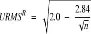(1)

Thus, from eq. (1) we can then compute a similarity score (S_AB) between any two heptapeptides A and B as:

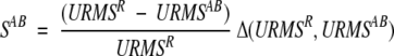(2)

Here, Δ(URMS^R, URMS^AB) = 10 if URMS^R > URMS^AB and Δ(URMS^R, URMS^AB) = 0 otherwise. Therefore, S_AB provides a similarity scale between 0 and 10. Entries S_AB are used to build the similarity matrix S obtained by comparing all possible heptapeptides in both proteins. Dynamic Programming is then applied to this similarity matrix in order to build an alignment of both structures on the basis of their backbone (local) similarity. This alignment is produced using a global alignment method with zero end gaps (Needleman and Wunsch 1970). Internal gaps are penalized using an affine gap penalty function of the form g(k) = α+βk, where k is the number of gaps and α and β are the opening and extension penalties, respectively. Trial and error tests (see below) indicated that values of α = 7.00 and β = 0.45 gave good results.

(3) Find the maximum subset of similar local structures that have their corresponding C α close in cartesian space. Close is considered here as a distance less than or equal to 4.0 Å. The method to find this subset is a small variant of the heuristic MaxSub algorithm (Siew et al. 2000; http://www.cs.bgu.ac.il/∼dfischer/MaxSub/). Once the algorithm converges, the percentage of structural identity (PSI) is computed, defined as the percentage of corresponding residues below 4.0 Å in 3D space, measured with respect to the shortest structure.

(4) Calculate the probability of obtaining the given proportion of aligned residues (with respect to the shortest protein model) by chance (P-value). The P-value estimation is based on extreme-value fitting of the scores resulting from random structural alignments, following the work of Abagyan and Batalov (1997). The Type-I extreme value distribution based on the largest extreme, also known as the Gumbel distribution, has the following general form for its probability density function (Gumbel 1958):

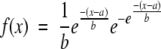(3)

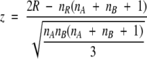
where a is the so-called location parameter and b is the scale parameter. We are interested in the probability of having a t value greater than x, P(t > x). This value can be found by integrating equation (3) from t to infinity, yielding:

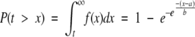(4)

In order to apply eq. (4) we need parameters a and b. For their derivation it is more convenient to work with the probability of having a value t smaller than or equal to x:

(5)

Taking logarithms in eq. (5) and setting Q(x) = P(t ≤ x) and P(x) = P(t > x), we have Q(x) + P(x) = 1. Equation 5 can then be transformed to the following linear form:

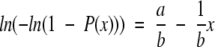(6)

Parameters a and b can now be estimated from a linear fitting between x, the percentage of aligned residues (PSI) obtained from the structural alignment algorithm in step 3, and ln(−ln(1−P(x))), where P(x) is computed as an accumulated sum of the observed frequencies with values greater than x. The reason for using P(x) instead of Q(x) in eq. 6 is in order to give a larger weight to the tail of the distribution, which contains the most critical part of the curve. Once a and b are found, expected values for the mean μ and variance σ² can be derived using the method of moments, giving relationships:

(7)

(8)

where γ ≈ 0.5772 is the well-known Euler-Mascheroni constant (Gumbel 1958). Introducing eqs. 10 and 11 in eq. 4, the P-value as a function of z-score is obtained:

(9)

Parameter optimization

Several parameters are used within the program: the length of the peptide in the URMS calculation, the similarity score derived from the URMS computation, the gap opening and extension penalties, the maximal distance between Cα, and the a and b parameters in the EVD. With the exception of the gap penalties and a and b parameters, no exhaustive optimization has been carried out. Gap penalties were optimized using a grid-like search, once the rest of parameters were fixed. The a and b parameters have been discussed previously. For the rest, values were initially established in order to avoid an undesirable combinatorial explosion in parameter space, based on the following considerations: (1) Number of residues for local similarity: This number has to be large enough to consider the different types of secondary structure. Four residues are required to define a helix turn and a β-turn. Thus, this would be a lower bound. However, calculations with ideal secondary structures (data not shown) indicated that helices and turns are difficult to distinguish by the URMS value with only four residues. Adding flanking residues provides a window of six residues, able to distinguish β-turns and helices. A seven-residue window was found to be more appropriate, however, probably because it can consider a complete two-helix turn. We observed that larger values begin to flat correct alignment pathways in similarity matrices, and therefore selected a heptapeptide. (2) Random URMS score: This value is established analytically, on the basis of the expected random values, and simply scaled between 0 and 10. Therefore there are no parameters to fit. (3) Maximal distance between Cα: Based on the value used in the MaxSub algorithm, together with visual observation of the results. The original MaxSub algorithm uses 3.5 Å. When dealing with models, a slightly larger value of 4 Å was deemed necessary.

Computation of coverage-error plots

From the all-versus-all comparison, we compute the coverage-error plot applying a procedure similar to that described by Levitt and Gerstein (1998): (1) For each pair we determine its P-value as computed by eq. 12, and note whether the pair is a true-positive or a true-negative; (2) We sort all pairs by increasing P-value; (3) We count down the list from best to worst and at each point in the list we find out the number of false positives and from that, the observed P-value; (4) We also compute the fraction of true positives that are more significant than the threshold P-value; this number defines the coverage, which should be as large as possible. On the other hand, observed and calculated P-values should be as close as possible.

Comparison with other evaluation methods

In order to assess the relative performance of MAMMOTH, we compared the evaluation scores provided by this approach with a set of 11 different evaluation methods previously used in CASP for structure comparison and model evaluation. All methods were benchmarked against the assumed gold standard given by Murzin’s manual ranking of models submitted to the CASP3 meeting (Murzin 1999). When assessing the merits of the different approaches discussed here, it is important to keep in mind that some of these algorithms were not specifically developed to compare predicted models with their corresponding experimental structures, but rather to compare and classify pairs of experimental structures. The following sets of automatic criteria for assessment of the different models were compared with that used by MAMMOTH:

1. During CASP3, Orengo (Orengo et al. 1999) evaluated the ab initio predictions using three different criteria: the amount of nonoverlapping segments of 25 residues with an RMS value of 4.0 Å (Lesk 1997, referenced here as orengo-lesk); the similarity of the structural environment at each residue position (Taylor and Orengo 1989; orengo-ssap); and the largest fragment with an RMS of 4.0 Å (Orengo et al. 1999; orengo-rmsd). All three measures were compared with the MAMMOTH score.

2. Dali (Holm and Sander 1993) is a well known program for protein structure comparison. The Dali Z-score has been frequently used in the evaluation of structural predictions (Ortiz et al. 1998b; Simons et al. 2001). We have studied here both the Z-score (dali) and the percentage of superimposed residues (dali-sup) provided by the DaliLite package (Holm and Park 2000).

3. Vast (Madej et al. 1995; Gibrat et al. 1996) is another automatic method frequently used for protein structural alignment. Vast scores were used in both CASP2 and CASP3 to evaluate predicted structures. Here we used as scores the RMSD of the structural alignment (vast-rmsd) and the percentage of superimposed residues (vast-sup).

4. PrISM (Yang and Honig 2000) is a recently reported multipurpose program for protein modeling that also evaluates structural relationships between protein structures by using a new measure of protein structural distance. We used as scores the protein structural distance (prism-psd); the secondary structure alignment score (prism-score) and the percentage of superimposed residues and calculated by PrISM.

5. Finally, the GDT method (Zemla et al. 1999) was also included. The score (gdt-ts) is obtained from the global distance test (Zemla et al. 1999). It takes into account the percentage of residues that can be found within a given distance threshold between model and target. The gdt-ts measure is an average of percentages obtained at 1, 2, 4, and 8 Å and has been used in previous assessments of CASP results by the Zemla team.

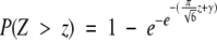
Comparisons were restricted to groups and targets evaluated jointly both by Murzin and Orengo during CASP3. These models are a subset of all models evaluated by Murzin during CASP3. The set of models included in the evaluation is listed in Table 3A of the Appendix. In order to test whether this subset is representative enough of the results that could have been obtained by using all models evaluated by Murzin, we used the Wilcoxon’s sum of ranks test (Langley 1970) using the Murzin, Dali, MAMMOTH, and PrISM scores (for which we had all scores for both sets). We then compared the set of Murzin evaluations (all models) with the set evaluated jointly by Orengo and Murzin (subset). Our null hypothesis was that there are no significant differences in score distribution between both sets of models, so that results of the subset are representative of the complete set in CASP3. The test is as follows (Langley 1970): First, the scores of both samples (Murzin’s set and the Orengo-Murzin subset) are pooled together. Then, the combined set of scores is sorted, and for each measurement a rank value is assigned. The smallest rank total R is then defined as the smaller of the sum of ranks coming from each sample. If distributions come from different underlying populations, unequal rank totals are expected. The probability of getting unequal rank totals as a consequence of chance variation can then be determined from R. The significance of the smaller rank total is found by calculating the statistic z given by the equation:

(10)

where n_R is the number of measurements in whichever sample possesses the smaller rank total. The z-statistic distributes normally under the null hypothesis, and therefore the significance of z can finally be calculated using a normal distribution (Langley 1970).

Table 3A.

Set of CASP3 models used to compare the different evaluation methods.

Models are available at http://predictioncenter.11n1.gov/casp3/Casp3.html

Selection of structural datasets

Fold set selected to compute the background random distribution (Table 1A, Appendix)

This set was used to fit the EVD and to obtain the P-value estimation. It comprises a set of different folds without significant sequence identity (25% cutoff in sequence identity), selected by combining the pdb_select list from Hobohm and coworkers (Hobohm et al. 1992; Hobohm and Sander 1994) with the SCOP database.

A test set selected to compute coverage error plots (Table 2A, Appendix)

In this test set we first selected a representative set of proteins of different folds as in the previous case, but in addition we incorporated for each fold a second representative.

Fold families

All fold families from SCOP with more than 15 members per family were selected. We were able to select families belonging to 115 different folds, with 22 of them from the all-α class, 24 from the all-β class, 20 from the α/β class, and 21 from the α+β class. The rest (18 folds) belongs to other classifications in SCOP.

Dataset of predicted models (Table 3A, Appendix)

Models were downloaded from the CASP web site at: http://predictioncenter.llnl.gov/casp3/Casp3.html.

References

- Abagyan, R. and Batalov, S. 1997. Do aligned sequences share the same fold? J. Mol. Biol. 273 355–368. [DOI] [PubMed] [Google Scholar]
- Adams, P.D. and Grosse-Kunstleve, R.W. 2000. Recent developments in software for the automation of crystallographic macromolecular structure determination. Curr. Opin. Struct. Biol. 10 564–568. [DOI] [PubMed] [Google Scholar]
- Al-Hashimi, H.M. and Patel, D.J. 2002. Residual dipolar couplings: Synergy between NMR and structural genomics. J. Biomol. NMR 22 1–8. [DOI] [PubMed] [Google Scholar]
- Baker, D. and Sali, A. 2001. Protein structure prediction and structural genomics. Science 294 93–96. [DOI] [PubMed] [Google Scholar]
- Bonneau, B., Strauss, C., Rohl, C., Chivian, D., Bradley, P., Malmstrom, L., Robertson, T., Baker, D. 2002. De novo prediction of three-dimensional structures for major protein families. J. Mol. Biol. 322 65. [DOI] [PubMed] [Google Scholar]
- Boutonnet, N.S., Rooman, M.J., Ochagavia, M.E., Richelle, J., and Wodak, S.J. 1995. Optimal protein structure alignments by multiple linkage clustering: Application to distantly related proteins. Protein Eng. 8 647–662. [DOI] [PubMed] [Google Scholar]
- Brenner, S.E. 2001. A tour of structural genomics. Nat. Rev. Genet. 2 801–809. [DOI] [PubMed] [Google Scholar]
- Burley, S.K. and Bonanno, J.B. 2002. Structural genomics of proteins from conserved biochemical pathways and processes. Curr. Opin. Struct. Biol. 12 383–391. [DOI] [PubMed] [Google Scholar]
- Chance, M.R., Bresnick, A.R., Burley, S.K., Jiang, J.S., Lima, C.D., Sali, A., Almo, S.C., Bonanno, J.B., Buglino, J.A., Boulton, S., et al. Structural genomics: A pipeline for providing structures for the biologist. Protein Sci. 11 723–738. [DOI] [PMC free article] [PubMed]
- Chew, L., Huttlenlocher, D., Kedem, K., and Kleinberg, J. 1999. Fast detection of common geometric substructure in proteins. J. Comput. Biol. 6 313–325. [DOI] [PubMed] [Google Scholar]
- Diller, D.J., Pohl, E., Redinbo, M.R., Hovey, B.T., and Hol, W.G. 1999a. A rapid method for positioning small flexible molecules, nucleic acids, and large protein fragments in experimental electron density maps. Proteins 36 512–525. [PubMed] [Google Scholar]
- Diller, D.J., Redinbo, M.R., Pohl, E., and Hol, W.G. 1999b. A database method for automated map interpretation in protein crystallography. Proteins 36 526–541. [PubMed] [Google Scholar]
- Domingues, F.S., Koppensteiner, W.A., and Sippl, M.J. 2000. The role of protein structure in genomics. FEBS Lett. 476 98–102. [DOI] [PubMed] [Google Scholar]
- Fetrow, J.S. and Skolnick, J. 1998. Method for prediction of protein function from sequence using the sequence-to-structure-to-function paradigm with application to glutaredoxins/thioredoxins and T1 ribonucleases. J. Mol. Biol. 281 949–968. [DOI] [PubMed] [Google Scholar]
- Fetrow, J.S., Godzik, A., and Skolnick, J. 1998. Functional analysis of the Escherichia coli genome using the sequence- to-structure-to-function paradigm: Identification of proteins exhibiting the glutaredoxin/thioredoxin disulfide oxidoreductase activity. J. Mol. Biol. 282 703–711. [DOI] [PubMed] [Google Scholar]
- Gibrat, J.F., Madej, T., and Bryant, S.H. 1996. Surprising similarities in structure comparison. Curr. Opin. Struct. Biol. 6 377–385. [DOI] [PubMed] [Google Scholar]
- Guda, C., Scheeff, E.D., Bourne, P.E., and Shindyalov, I.N. 2001. A new algorithm for the alignment of multiple protein structures using Monte Carlo optimization. Pac. Symp. Biocomput. 275–286. [DOI] [PubMed]
- Gumbel, E. 1958. Statistics of extremes. Columbia University Press, New York.
- Hobohm, U. and Sander, C. 1994. Enlarged representative set of protein structures. Protein Sci. 3 522–524. [DOI] [PMC free article] [PubMed] [Google Scholar]
- Hobohm, U., Scharf, M., Schneider, R., and Sander, C. 1992. Selection of representative protein data sets. Protein Sci. 1 409–417. [DOI] [PMC free article] [PubMed] [Google Scholar]
- Holm, L. and Park, J. 2000. DaliLite workbench for protein structure comparison. Bioinformatics 16 566–567. [DOI] [PubMed] [Google Scholar]
- Holm, L. and Sander, C. 1993. Protein structure comparison by alignment of distance matrices. J. Mol. Biol. 233 123–138. [DOI] [PubMed] [Google Scholar]
- ———1996. Mapping the protein universe. Science 273 595–603. [DOI] [PubMed] [Google Scholar]
- ——— 1998. Dictionary of recurrent domains in protein structures. Proteins 33 88–96. [DOI] [PubMed] [Google Scholar]
- Hurley, J.H., Anderson, D.E., Beach, B., Canagarajah, B., Ho, Y.S., Jones, E., Miller, G., Misra, S., Pearson, M., Saidi, L., Suer, S., Trievel, R., and Tsujishita, Y. 2002. Structural genomics and signaling domains. Trends Biochem. Sci. 27 48–53. [DOI] [PubMed] [Google Scholar]
- Jiang, W., Baker, M.L., Ludtke, S.J., and Chiu, W. 2001. Bridging the information gap: Computational tools for intermediate resolution structure interpretation. J. Mol. Biol. 308 1033–1044. [DOI] [PubMed] [Google Scholar]
- Johnson, R. and Wichern, D. 1998. Applied multivariate statistical analysis. Prentice Hall, Upper Saddle City, New Jersey.
- Jung, J. and Lee, B. 2000. Protein structure alignment using environmental profiles. Protein Eng. 13 535–543. [DOI] [PubMed] [Google Scholar]
- Kedem, K., Chew, L., and Elber, R. 1999. Unit-vector RMS (URMS) as a tool to analyze molecular dynamics trajectories. Proteins 37 554–564. [PubMed] [Google Scholar]
- Kleywegt, G.J. 1999. Recognition of spatial motifs in protein structures. J. Mol. Biol. 285 1887–1897. [DOI] [PubMed] [Google Scholar]
- Labesse, G., Colloc’h, N., Pothier, J., and Mornon, J.P. 1997. P-SEA: A new efficient assignment of secondary structure from C α trace of proteins. Comput. Appl. Biosci. 13 291–295. [DOI] [PubMed] [Google Scholar]
- Lackner, P., Koppensteiner, W.A., Sippl, M.J., and Domingues, F.S. 2000. ProSup: A refined tool for protein structure alignment. Protein Eng. 13 745–752. [DOI] [PubMed] [Google Scholar]
- Lamzin, V.S. and Perrakis, A. 2000. Current state of automated crystallographic data analysis. Nat. Struct. Biol. 7 978–981. [DOI] [PubMed] [Google Scholar]
- Langley, R. 1970. Practical statistics. Simply explained. Dover, New York.
- Leibowitz, N., Fligelman, Z.Y., Nussinov, R., and Wolfson, H.J. 2001a. Automated multiple structure alignment and detection of a common substructural motif. Proteins 43 235–245. [DOI] [PubMed] [Google Scholar]
- Leibowitz, N., Nussinov, R., and Wolfson, H.J. 2001b. MUSTA—A general, efficient, automated method for multiple structure alignment and detection of common motifs: Application to proteins. J. Comput. Biol. 8 93–121. [DOI] [PubMed] [Google Scholar]
- Lesk, A. 1997. CASP2: Report on ab initio predictions. Proteins 1 151–166. [DOI] [PubMed] [Google Scholar]
- Levitt, M. and Gerstein, M. 1998. A unified statistical framework for sequence comparison and structure comparison. Proc. Natl. Acad. Sci. 95 5913–5920. [DOI] [PMC free article] [PubMed] [Google Scholar]
- Lichtarge, O. and Sowa, M.E. 2002. Evolutionary predictions of binding surfaces and interactions. Curr. Opin. Struct. Biol. 12 21–27. [DOI] [PubMed] [Google Scholar]
- Lo Conte, L., Ailey, B., Hubbard, T.J., Brenner, S.E., Murzin, A.G., and Chothia, C. 2000. SCOP: A structural classification of proteins database. Nucleic Acids Res. 28 257–259. [DOI] [PMC free article] [PubMed] [Google Scholar]
- Madabushi, S., Yao, H., Marsh, M., Kristensen, D.M., Philippi, A., Sowa, M.E., and Lichtarge, O. 2002. Structural clusters of evolutionary trace residues are statistically significant and common in proteins. J. Mol. Biol. 316 139–154. [DOI] [PubMed] [Google Scholar]
- Madej, T., Gibrat, J.F., and Bryant, S.H. 1995. Threading a database of protein cores. Proteins 23 356–369. [DOI] [PubMed] [Google Scholar]
- McLachlan, A.D. 1979. Gene duplications in the structural evolution of chymotrypsin. J. Mol. Biol. 128 49–79. [DOI] [PubMed] [Google Scholar]
- Mittl, P.R. and Grutter, M.G. 2001. Structural genomics: Opportunities and challenges. Curr. Opin. Chem. Biol. 5 402–408. [DOI] [PubMed] [Google Scholar]
- Moult, J., Hubbard, T., Fidelis, K., and Pedersen, J.T. 1999. Critical assessment of methods of protein structure prediction (CASP): Round III. Proteins l 2–6. [PubMed] [Google Scholar]
- Murzin, A.G. 1999. Structure classification-based assessment of CASP3 predictions for the fold recognition targets. Proteins l 88–103. [DOI] [PubMed] [Google Scholar]
- Murzin, A.G., Brenner, S.E., Hubbard, T., and Chothia, C. 1995. SCOP: A structural classification of proteins database for the investigation of sequences and structures. J. Mol. Biol. 247 536–540. [DOI] [PubMed] [Google Scholar]
- Needleman, S. and Wunsch, C. 1970. A general method applicable to the search for similarities in the amino acid sequence of two proteins. J. Mol. Biol. 48 443–453. [DOI] [PubMed] [Google Scholar]
- Orengo, C., Bray, J., Hubbard, T., LoConte, L., and Sillitoe, I. 1999. Analysis and assessment of ab initio three-dimensional prediction, secondary structure, and contacts prediction. Proteins 37 149–170. [DOI] [PubMed] [Google Scholar]
- Ortiz, A.R., Kolinski, A., and Skolnick, J. 1998a. Fold assembly of small proteins using monte carlo simulations driven by restraints derived from multiple sequence alignments. J. Mol. Biol. 277 419–448. [DOI] [PubMed] [Google Scholar]
- Ortiz, A.R., Kolinski, A., and Skolnick, J. 1998b. Nativelike topology assembly of small proteins using predicted restraints in Monte Carlo folding simulations. Proc. Natl. Acad. Sci. 95 1020–1025. [DOI] [PMC free article] [PubMed] [Google Scholar]
- Ortiz, A.R., Kolinski, A., Rotkiewicz, P., Ilkowski, B., and Skolnick, J. 1999. Ab initio folding of proteins using restraints derived from evolutionary information. Proteins (Suppl 3): 177–185. [DOI] [PubMed]
- Perrakis, A., Morris, R., and Lamzin, V.S. 1999. Automated protein model building combined with iterative structure refinement. Nat. Struct. Biol. 6 458–463. [DOI] [PubMed] [Google Scholar]
- Prestegard, J.H., Valafar, H., Glushka, J., and Tian, F. 2001. Nuclear magnetic resonance in the era of structural genomics. Biochemistry 40 8677–8685. [DOI] [PubMed] [Google Scholar]
- Reddy, B.V., Li, W.W., Shindyalov, I.N., and Bourne, P.E. 2001. Conserved key amino acid positions (CKAAPs) derived from the analysis of common substructures in proteins. Proteins 42 148–163. [DOI] [PubMed] [Google Scholar]
- Sali, A. 1998. 100,000 protein structures for the biologist. Nat. Struct. Biol. 5 1029–1032. [DOI] [PubMed] [Google Scholar]
- Sander, C. and Schneider, R. 1991. Database of homology-derived protein structures and the structural meaning of sequence alignment. Proteins 9 56–68. [DOI] [PubMed] [Google Scholar]
- Shindyalov, I.N. and Bourne, P.E. 1998. Protein structure alignment by incremental combinatorial extension (CE) of the optimal path. Protein Eng. 11 739–747. [DOI] [PubMed] [Google Scholar]
- Shindyalov, I.N. and Bourne, P.E. 2000. An alternative view of protein fold space. Proteins 38 247–260. [PubMed] [Google Scholar]
- Siew, N., Elofsson, A., Rychlewski, L., and Fischer, D. 2000. MaxSub: An automated measure for the assessment of protein structure prediction quality. Bioinformatics 16 776–785. [DOI] [PubMed] [Google Scholar]
- Simons, K.T., Bonneau, R., Ruczinski, I.I., and Baker, D. 1999. Ab initio protein structure prediction of CASP III targets using ROSETTA. Proteins 37 171–176. [DOI] [PubMed] [Google Scholar]
- Simons, K.T., Strauss, C., and Baker, D. 2001. Prospects for ab initio protein structural genomics. J. Mol. Biol. 306 1191–1199. [DOI] [PubMed] [Google Scholar]
- Taylor, W. and Orengo, C. 1989. Protein structure alignment. J. Mol. Biol. 208 1–22. [DOI] [PubMed] [Google Scholar]
- Teichmann, S.A., Murzin, A.G., and Chothia, C. 2001. Determination of protein function, evolution and interactions by structural genomics. Curr. Opin. Struct. Biol. 11 354–363. [DOI] [PubMed] [Google Scholar]
- Thornton, J. 2001. Structural genomics takes off. Trends Biochem. Sci. 26 88–89. [DOI] [PubMed] [Google Scholar]
- Thornton, J.M., Todd, A.E., Milburn, D., Borkakoti, N., and Orengo .A. 2000. From structure to function: Approaches and limitations. Nat. Struct. Biol. 7, 991–994. [DOI] [PubMed] [Google Scholar]
- Vitkup, D., Melamud, E., Moult, J., and Sander, C. 2001. Completeness in structural genomics. Nat. Struct. Biol. 8 559–566. [DOI] [PubMed] [Google Scholar]
- Yang, A. and Honig, B. 2000. An integrated approach to the analysis and modeling of protein sequences and structures. I. Protein structural alignment and a quantitative measure for protein structural distance. J. Mol. Biol. 301 665–678. [DOI] [PubMed] [Google Scholar]
- Zemla, A., Venclovas, C., Moult, J., and Fidelis, K. 1999. Processing, and analysis of CASP3 protein structure predictions. Proteins Suppl (3) 22–29. [DOI] [PubMed]