

Abstract
The more proteins diverged in sequence, the more difficult it becomes for bioinformatics to infer similarities of protein function and structure from sequence. The precise thresholds used in automated genome annotations depend on the particular aspect of protein function transferred by homology. Here, we presented the first large-scale analysis of the relation between sequence similarity and identity in subcellular localization. Three results stood out: (1) The subcellular compartment is generally more conserved than what might have been expected given that short sequence motifs like nuclear localization signals can alter the native compartment; (2) the sequence conservation of localization is similar between different compartments; and (3) it is similar to the conservation of structure and enzymatic activity. In particular, we found the transition between the regions of conserved and nonconserved localization to be very sharp, although the thresholds for conservation were less well defined than for structure and enzymatic activity. We found that a simple measure for sequence similarity accounting for pairwise sequence identity and alignment length, the HSSP distance, distinguished accurately between protein pairs of identical and different localizations. In fact, BLAST expectation values outperformed the HSSP distance only for alignments in the subtwilight zone. We succeeded in slightly improving the accuracy of inferring localization through homology by fine tuning the thresholds. Finally, we applied our results to the entire SWISS-PROT database and five entirely sequenced eukaryotes.
Keywords: Protein function, evolution, sequence conservation threshold, subcellular localization, homolog detection, prediction by homology
Sequence conservation of protein function.
Proteins retain the memory of their evolutionary ancestry in their sequence, structure, and function. High-sequence similarity alone is considered to be sufficient evidence for common ancestry and is routinely used to infer structural and functional similarity (Bork and Koonin 1998). However, many proteins of similar structure have no discernible sequence similarity (Rost 1997, 1999; Murzin 1998; Yang and Honig 2000b). The evolutionary conservation of protein structure, that is, the relationship between similarity in sequence and in structure has been explored extensively (Chothia and Lesk 1986; Sander and Schneider 1991; Abagyan and Batalov 1997; Alexandrov and Soloveyev 1998; Brenner et al. 1998; Park et al. 1998; Jaroszewski et al. 2000; Blake and Cohen 2001). The resulting thresholds enable transferring structural annotations (Sander and Schneider 1991; Teichmann et al. 1998, 1999; Liu and Rost 2001; Vitkup et al. 2001; J. Liu and B. Rost, in prep.). The thresholds for sequence similarity that imply similarity in function cannot be inferred from those for structure (Shah and Hunter 1997; Devos and Valencia 2000, 2001; Pawlowski et al. 2000; Wilson et al. 2000; Todd et al. 2001; Rost 2002). One problem in establishing thresholds for the transfer of function is that the term "protein function"—albeit intuitive—is not well defined. Function is a complex phenomenon associated with many mutually overlapping levels, chemical, biochemical, cellular, organism mediated, and developmental. These levels are related in complex ways; for example, protein kinases can be related to different cellular functions (such as cell cycle), and to a chemical function (transferase) plus a complex control mechanism by interaction with other proteins. This lack of a precise definition generates two specific problems for analyzing the conservation of function. First, we have sufficiently large, machine-readable data only for very few aspects of function (Wilson et al. 2000). Second, the conservation differs significantly between different types of function (Devos and Valencia 2000; Pawlowski et al. 2000; Wilson et al. 2000; Todd et al. 2001; Rost 2002). Nevertheless, a better understanding of the relation between function and sequence is fundamentally important, because it can provide insights into the underlying mechanisms of evolving new functions through changes in sequence and structure (Thornton et al. 1999). Large-scale genome sequencing projects have led to a rapidly widening gap between the number of known sequences and their functional annotations. Efforts at addressing this situation have largely relied on exploiting sequence similarity to infer functional similarity (Koonin et al. 1994; Casari et al. 1995; Ouzounis et al. 1996; Schneider et al. 1997; Bork and Koonin 1998; Tamames et al. 1998; Andrade et al. 1999; Koonin 2000). However, few large-scale studies have evaluated the accuracy of the transfer of function (Eisenhaber and Bork 1998; Karp 1998; Devos and Valencia 2000, 2001; Rost 2002).
Three zones of sequence comparisons: From trivial (safe) over problematic (twilight) to impossible (midnight).
In general, we can separate between three regions of protein comparisons (Fig. 1 ▶) as follows: (1) safe zone: For very high levels of sequence similarity proteins have similar functions and structures—aligning the proteins is straightforward; (2) twilight zone (Doolittle 1986): At some point of divergence, the alignment of proteins becomes problematic; in fact, we no longer can safely infer similarity in a particular feature from sequence. However, typically, a considerable fraction of the protein pairs identified in the twilight zone still have a particular feature in common; and (3) midnight zone: Protein pairs in this zone have levels of sequence similarity so low that we can no longer detect their similarity from sequence alone (Rost 1997, 1999). Interestingly, the vast majority of protein pairs with similar three-dimensional structure populate the midnight zone (Rost 1997, 1998; Brenner et al. 1998; Yang and Honig 2000b).
Fig. 1.

Transition from safe over twilight to midnight zone of protein comparisons. Alignment methods maximize the sequence similarity between two proteins. When we want to translate these levels of sequence similarity to conclusions about similarity in structure/function, we can distinguish three major regions; the boundaries between these are not well defined. (1) Safe zone: All protein pairs in this region have similar structure/function, that is, sequence similarity implies similarity in structure/function. (2) Twilight zone: Most pairs in this region have similar structure/function. (3) Midnight zone: Whereas many of the pairs in this region may have similar structure/function, most do not. The curves illustrate accuracy (or specificity, black line) and coverage (or selectivity, grey line); the x-axis gives the pairwise sequence similarity, the y-axis the percentage of pairs that are similar above the given threshold (accuracy) and the percentage of similar pairs that are found above the given threshold (coverage). These sketched curves point out that there is a trade off between accuracy and coverage; whereas the safe zone is defined by 100% accuracy, we typically find only a few of the pairs with similar structure/function in this region of sequence similarity (low coverage). On the other extreme end, we find many pairs of similar structure/function in the midnight zone (high coverage). However, the accuracy is very low. Obviously, the choice of appropriate thresholds constitutes a balance between the Skylla of 100% accuracy, no homolog found and the Charibdis of many putative homologs found, most are not homologous. The particular shape of the curves that describe accuracy and coverage depends on the problem at hand, that is, on the particular feature of biological similarity that we try to infer (Fig. 6 ▶ compares the transition for a variety of features). Here, we focus on the problem of establishing thresholds that allow inferring subcellular localization through sequence similarity.
Statistical scores versus percentage sequence identity for conservation of structure.
The most popular database search methods BLAST and PSI-BLAST (Altschul et al. 1990, 1997; Altschul 1993) use neither percent sequence identity nor raw alignment scores to characterize sequence similarity. Instead, they use probabilities or expectation values that reflect the statistical significance of a given alignment. It has been claimed that statistical scoring schemes are superior to scores on the basis of pairwise sequence identity in identifying structural homologs (Pearson 1995; Abagyan and Batalov 1997; Brenner et al. 1998; Park et al. 1998; Wood and Pearson 1999). Statistical scores are clearly superior to simply measuring pairwise sequence identity. Sander and Schneider (1991) introduced another measure for sequence similarity to identify proteins of similar structure when building their HSSP database. Their measure, the HSSP distance correlates alignment length and pairwise sequence identity. A minor modification of the original HSSP curve resulted in a measure for sequence similarity that appears more successful than statistical scores in describing structural similarity for pairwise alignments (Rost 1999). Can we generalize the lessons learned from the conservation of structure to that of function?
Sharp transition of thresholds describing the sequence conservation of function.
Recent efforts at investigating the sequence-function relation have utilized three different classifiers for function as follows: (1) enzymatic activity as described by the Enzyme Commission (EC; Webb 1992) numbers (Shah and Hunter 1997; Hegyi and Gerstein 1999; Devos and Valencia 2000; Pawlowski et al. 2000; Wilson et al. 2000; Todd et al. 2001; Rost 2002); (2) SWISS-PROT keywords (Devos and Valencia 2000); and (3) the GeneOntology (GO; Lewis et al. 2000) classification as used in FLYBASE (Ashburner and Drysdale 1994; Wilson et al. 2000). Wilson et al. (2000) observed that the separation between proteins of similar and nonsimilar function is best described by sigmoidal curves that drop off sharply at particular thresholds for conservation. They claimed near-perfect conservation of function as measured by EC and GO above 40%–50% pairwise sequence identity. Other groups have published similar findings for enzymatic activity (Shah and Hunter 1997; Devos and Valencia 2000; Pawlowski et al. 2000; Todd et al. 2001). More recently, we have found that most of these results appeared overoptimistic, that is, that enzymatic function is less well conserved than anticipated (Rost 2002). Devos and Valencia (2000) have also investigated the sequence identity-to-function relationship for SWISS-PROT (Bairoch and Apweiler 2000) keywords and binding sites. Whereas they find that the functional shapes of the threshold separating conserved and nonconserved function are similar between different aspects of function, the precise thresholds differ between EC, keywords, and binding sites. In contrast to all other groups, Pawlowski et al. (2000) reported thresholds for conservation that were not sharp. Their measure of sequence similarity was based on their in-house alignment program BASIC (Rychlewski et al. 1999).
Statistical scores versus percentage sequence identity for conservation of function.
Wilson et al (2000) found percent identity to be better at quantifying functional similarity than statistical scoring schemes. However, their results also indicated that statistical scoring schemes are better at discriminating between highly diverged sequences. In contrast, Pawlowski et al. (2000) and our recent results (Rost 2002) suggested that both statistical Z-scores and BLAST expectation values were clearly superior to pairwise sequence identity at quantifying similarity in enzymatic function. However, our results also confirmed that a combination of alignment length and pairwise sequence identity outperforms BLAST scores at levels of low-sequence divergence (Rost 2002).
Sequence conservation of subcellular localization.
The subcellular localization of a protein is correlated with its function (Ferrigno and Silver 1999; Faust and Montenarh 2000; Pearce 2000). Obviously, we expect proteins with very similar sequences to be localized in similar cellular compartments. In fact, this assumption is applied in everyday sequence analysis and database annotations (Eisenhaber and Bork 1998; Bairoch and Apweiler 2000). However, although we do know that subcellular localization is evolutionarily imprinted onto the protein surface (Andrade et al. 1998), the precise threshold for the sequence conservation of subcellular localization has not been explored yet. Here, we investigated this conservation for different compartments, that is, implicitly for different aspects of function (Liscovitch et al. 1999; Sirover 1999). Using subcellular localization to quantify functional similarity, we rediscovered particular features of the sequence-function relationship noticed for other types of function before (Shah and Hunter 1997; Devos and Valencia 2000; Jaroszewski et al. 2000; Pawlowski et al. 2000; Wilson et al. 2000; Todd et al. 2001;Rost 2002). We benchmarked the effectiveness of various scoring schemes and proposed a new scheme for refined identification of functional homologs and compared the accuracy of homology transfer with the accuracy of prediction methods (Claros et al. 1997; Nielsen et al. 1999; Drawid and Gerstein 2000; Nakai 2001). Finally, we applied our scheme to annotate five entirely sequenced eukaryotes and the entire SWISS-PROT database. In conjunction with other studies relating structure-to-function, our work provided useful insights into the evolution of new functions through sequence and structural changes. Our results may lead to improvements in functional annotations of newly sequenced genomes.
Results
Over one million pair comparisons between proteins of known localization.
The data set of proteins with experimentally known subcellular localization extracted from SWISS-PROT contained 7405 proteins. Because many of these proteins were very similar in sequence (bias), we constructed a representative sequence-unique subset containing 1248 proteins (Table 1). Our objective was to establish at which level of sequence similarity proteins reside in the same localization. To obtain estimates that are unbiased, we have to analyze the unbiased, sequence-unique set. However, if we were to align an all-against-all for subset of 1248, we would not find any close homologs, as by construction, no pair in the sequence-unique set is closely related. Consequently, we could not deduce thresholds for everyday sequence comparisons. Therefore, we have to accept some bias by aligning all proteins from the sequence-unique set against all proteins from the full set. Thus, our results were based on over nine million pair comparisons. Although this number might appear high enough to allow statements about statistical significance, the data set was not evenly distributed between the 11 different compartments (Table 1). We distinguished between major compartments (nucleus, cytoplasm, mitochondria, extra-cellular space, and chloroplasts), for which we had sufficiently large sets, and minor compartments (vacuoles, Golgi, and periplasm), for which the sets were too small to generalize our findings. Three compartments (lysosome, ER, and peroxysome) ranged somewhere in between these two extremes.
Table 1.
Experimentally annotated subcellular localization data from SWISS-PROT
| Subcellular localization | All SWISS-PROTa | Sequence-uniqueb |
| Nucleus | 2642 | 490 |
| Cytoplasm | 2161 | 326 |
| Mitochondria | 812 | 160 |
| Extra-cellular space | 663 | 107 |
| Chloroplast | 943 | 84 |
| Lysosome | 112 | 26 |
| Endoplasmic reticulum (ER) | 125 | 20 |
| Peroxysome | 94 | 18 |
| Vacuoles | 35 | 13 |
| Golgi apparatus | 14 | 4 |
| Periplasm | 4 | 0 |
| SUM (all 11) | 7405 | 1248 |
a Number of proteins with known localization found in SWISS-PROT.
b Number of sequence-unique proteins, i.e., representative subset of all SWISS-PROT proteins (Materials and Methods).
Sequence conservation of localization similar for major compartments.
The functional shapes for the sequence conservation of subcellular localization were similar across the major compartments (Fig. 2 ▶). The thresholds for accurate inference of localization through homology were around HSSP distances of 4 (Eq. 1; Fig. 2A ▶). We observed similar functional behavior for alignments generated using pairwise BLAST (Fig. 2A ▶) and PSI-BLAST profiles (Fig. 2B ▶) for the alignment. The cumulative coverage (Eq. 4), however, showed considerable variation for pairs belonging to the different localizations. Remarkably, the transition from safe zone to twilight zone (Fig. 1 ▶) occurred at an HSSP distance close to that for the sequence conservation of protein structure (HSSP distance of 0; Rost 1999; Fig. 2 ▶).
Fig. 2.

Sequence conservation for major classes of subcellular localization. For different thresholds in terms of the HSSP distance (Eq. 1), we compiled the levels of cumulative accuracy (Eq. 3) and cumulative coverage (Eq. 4). The major compartments had very similar curves for cumulative accuracy. The transition from the safe zone to the twilight zone occurred around HSSP distances of 4. In contrast to the perfect conservation of structure, the cumulative accuracy (A) was observed to be as low as 80% (for mitochondrial proteins) in the safe zone. The cumulative coverage (B) showed greater variation among the different compartments; the transition for coverage occurred between HSSP distance 5 and −5. The coverage remained significantly low even at very low levels of accuracy.
Sharp transition from safe to twilight zone.
If we want to infer the localization of a protein through homology to a protein of experimentally known localization, we have to relate sequence similarity to the conservation of the compartment. We explored three different ways of measuring sequence similarity (see Materials and Methods). (1) BLAST expectation values (E-VAL; Altschul and Gish 1996); (2) percentage pairwise sequence identity (PIDE); and (3) the distance from the HSSP threshold (DIST, Eq. 1). The curves describing the sequence conservation of localization resembled sigmoidal relationships (Fig. 3 ▶). Similar functional shapes describe the sequence conservation of enzymatic activity (Wilson et al. 2000; Todd et al. 2001; Rost 2002), of gene ontology classes (Wilson et al. 2000), and of protein structure (Vogt et al. 1995; Abagyan and Batalov 1997; Brenner et al. 1998; Park et al. 1998; Rost 1999; Jaroszewski et al. 2000; Blake and Cohen 2001). The conservation of localization (Fig. 3 ▶) was characterized by a region of slow monotonic decrease in accuracy (safe zone), followed by a transition to a region in which the accuracy decreases sharply (twilight/midnight zones). The transition from safe to twilight zone was markedly sharper for the BLAST expectation values (Fig. 3B,E) and for the HSSP distance (Fig. 3C,F) than for pairwise sequence identity (Fig. 3A,D). Similar results have been reported for structure (Yang and Honig 2000a). The curves relating accuracy (Eq. 3; data not shown) and cumulative accuracy (Eq. 3; Fig. 3 ▶), respectively, to sequence similarity were rather similar. The results for the biased and unique data sets were surprisingly similar for the HSSP distance and the BLAST expectations values (Fig. 3 ▶). However, the results differed significantly for pairwise sequence identity (Fig. 3A,D); the biased set suggested that we can correctly infer localization through homology for 90% of all proteins if we require about 50% identical residues (Fig. 3A ▶). This is similar to what many molecular biologists would use in everyday sequence analysis. In contrast, the sequence-unique set indicated that we need over 70% identical residues to correctly infer localization at a level of 90% accuracy for pairwise BLAST searches (Fig. 3D ▶).
Fig. 3.

Average conservation of subcellular localization. Graphs A, B, C show the performance of pairwise BLAST searches for the biased set, whereas graphs D, E, F show the performance of pairwise BLAST and PSI-BLAST searches on the sequence-unique subset. The filled symbols show cumulative accuracy and cumulative coverage (Eq. 3) for pairwise BLAST; open symbols give the results from PSI-BLAST searches. For the biased set, the cumulative coverage is 1% corresponding to the identification of ∼274K pairs from identical localization (true pairs), whereas for the sequence-unique subset, a cumulative coverage of 1% corresponds to the identification of ∼21K true pairs. Conservation thresholds for BLAST and PSI-BLAST are indicated by open and filled arrows, respectively. For HSSP distance (C,F), the conservation threshold using BLAST was at HSSP distance = 4 (open arrow) for the biased and sequence-unique sets, whereas by using PSI-BLAST, the conservation threshold was at HSSP distance = 0 (filled arrow) for the sequence-unique set. The cumulative accuracy and cumulative coverage when using BLAST for the sequence-unique set was 87% and 0.36%, respectively, and for PSI-BLAST, it was 91% and 0.4%, respectively. For the cumulative accuracy vs percent sequence identity graphs (A,D), no sharp conservation thresholds could be established. The percent sequence identity graphs showed the largest variation for the biased and sequence-unique sets. In contrast, the graphs for BLAST E-values (B,E) and HSSP distances (C,F, Eq. 1) were similar for the biased and the sequence-unique set. The conservation thresholds for PSI-BLAST occurred at a lower threshold than that for pairwise BLAST (D,E,F). The middle graphs plot the logarithm of the BLAST E-values (log to the base e). Note that BLAST E-values below 10−200 did not suffice to safely infer localization. In contrast, at very high HSSP distances and sequence identities, localization could be reliably transferred.
Expectation values outperformed HSSP distance for very diverged pairs.
When analyzing the relation between accuracy (percentage of localizations correctly inferred above given threshold) and coverage (number of correct inferences made above threshold), we noticed that the HSSP distance outperformed simple pairwise sequence identity for all thresholds (Fig. 4A ▶, circles vs. squares). However, the HSSP distance was superior to the BLAST expectation values only for proteins of conserved structure (HSSP distances above 0, Fig. 4A ▶, circles vs. diamonds, pairwise BLAST transition marked by top, left arrow). Surprisingly, the BLAST expectation values were slightly inferior to percentage pairwise sequence identity for very similar proteins (Fig. 4A ▶ indicated by bottom, right-hand arrow). For PSI-BLAST, percent sequence identity performed even better. Because the HSSP distance gave the best prediction above the conservation threshold (Fig. 4A ▶), using HSSP distances to infer localization by homology improves the accuracy of information transfer significantly. In fact, the HSSP curve derived to describe the sequence conservation of protein structure (Rost 1999), described the basic difference between protein pairs of identical and of different localizations surprisingly well (Fig. 5 ▶). We obtained similar graphs for the individual localizations and for PSI-BLAST profiles (data not shown).
Fig. 4.

Performance for different measures of sequence similarity. The black lines and open symbols show cumulative coverage vs cumulative accuracy for PSI-BLAST searches, whereas grey lines and shaded symbols show the same for pairwise BLAST (A,B). The figure plots data only for cumulative accuracy above 80%, which is well below the threshold for conservation of localization. (A) For HSSP distance (circles) and percent sequence identity (squares), PSI-BLAST vastly outperforms pairwise BLAST. However, using BLAST E-values, both BLAST and PSI-BLAST gave comparable performance at the conservation threshold (86% cumulative accuracy in figure). For both pairwise BLAST and PSI-BLAST, scoring the alignments using HSSP distance (Eq. 1) gave the best coverage vs accuracy graphs. Using HSSP distance for PSI-BLAST, alignments gave overall best performance. (B) For both pairwise BLAST and PSI-BLAST, using scaled distance (Eq. 2) from the HSSP curve improved performance compared with HSSP distance. The performance was worse when perpendicular distance from the HSSP curve was used. Overall, using PSI-BLAST alignments and scaled distance from the HSSP curve gave best performance. The curves for cumulative accuracy and coverage for the scaled HSSP distance (C) were similar to those obtained for the standard HSSP distance (Fig. 3F ▶).
Fig. 5.

Percentage pairwise sequence identity vs. length of alignment. The grey plus signs represent protein pairs experimentally observed in identical compartments, whereas the black squares represent pairs observed in different compartments. The grey line is the HSSP curve (Eq. 1) optimized to describe the sequence conservation of protein structure (Rost 1999). The HSSP curve was surprisingly accurate at reproducing the curve that may best separate proteins with identical localization from those of different localization.
Refining the thresholds to infer localization by homology.
We might improve the accuracy of transferring experimental information about localization by homology in two ways. We could refine the original HSSP curve used to determine the thresholds for this inference. However, the incorrect predictions shown in Figure 5 ▶ suggested that this might not be simple. Alternatively, we could modify the way of compiling the distance from the HSSP curve used to establish thresholds. Toward this end, we explored the following alternatives: (1) standard HSSP-distance (Eq. 1, note that this is the distance used for all previous figures), (2) perpendicular HSSP distance (Materials and Methods), and (3) a scaled HSSP distance (Eq. 2). We found the scaled HSSP distance slightly superior to the standard HSSP distance, whereas the perpendicular HSSP distance performed significantly worse (Fig. 4B ▶). For pairwise BLAST searches, the scaled HSSP distance discovered 13% more pairs of identical localization than the standard HSSP distance at the same conservation threshold. The curves relating cumulative accuracy and cumulative coverage, respectively, to scaled HSSP distance (Fig. 4C ▶) were similar to those obtained for HSSP distance (Fig. 3F ▶).
Annotation transfer for entire SWISS-PROT and entire eukaryotes.
Using the scaled HSSP distance (Eq. 2), we annotated the subcellular localization on the basis of homology for approximately one-fifth of the proteins in five entirely sequenced eukaryotes and the entire SWISS-PROT database (Table 2). The percentages of proteins for which we could infer localization differed substantially between the highest value above 26% for human and the lowest around 13% for the worm. Previously, we predicted that ∼20% of all fly proteins are nuclear (Cokol et al. 2000). In contrast, >60% of all the proteins for which we could infer localization by homology for entire proteomes were nuclear. Obviously, this number reflected the current bias. The annotations of subcellular localization are available at http://cubic.bioc.columbia.edu/db/LocHom/.
Table 2.
Inferring subcellular localization by homology
| Percentage of homology inferrede | |||||||||
| Data seta | Nprotb | Nhomoc | Phomod | nuc | cyt | ext | mit | pla | mis |
| Arabidopsis thaliana (plant) | 25456 | 3997 | 15.7 | 62 | 11 | 11 | 5 | 5 | 7 |
| Caenorhabditis elegans (worm) | 18898 | 2478 | 13.1 | 68 | 8 | 13 | 6 | <1 | 5 |
| Drosophila melanogaster (fly) | 14184 | 3033 | 21.4 | 67 | 10 | 13 | 5 | <1 | 4 |
| Mus musculus (mouse) | 28096 | 7496 | 26.7 | 65 | 15 | 11 | 5 | <1 | 4 |
| Homo sapiens (human) | 31073 | 8216 | 26.4 | 62 | 14 | 16 | 4 | <1 | 3 |
| SWISS-PROT | 109381 | 26651 | 24.4 | 35 | 19 | 17 | 14 | 9 | 5 |
a Data set: Entirely sequenced eukaryotic organisms and the SWISS-PROT database.
b Nprot: number of proteins in the database.
c Nhomo: number of proteins for which localization could be predicted using homology at more than 70 percent accuracy (only alignments with scaled HSSP-distance >4 retained, see Materials and Methods).
d Panno: percentage of proteins annotated (100*Nhomo/Nprot).
e Percentages of homology inferred proteins by compartment (= 100*Nx/Nhomo), with x = nuc (nuclear), = cyt (cytoplasmic), = ext (secreted to extra-cellular space), = mit (mitochondrial), = pla (chloroplast), and = mis (proteins predicted in one of the other localizations). Other localizations include lysosome, peroxysome, Endoplasmic reticulum, vacuoles, Golgi, and periplasm.
Ab initio prediction methods were not necessarily more accurate.
The accuracy of inferring subcellular localization by homology exceeded 80% at the HSSP distances of 4 (Fig. 2 ▶). We compared the performance of three publicly available prediction methods on the same sequence-unique data set. Note that the resulting estimates for prediction accuracy are likely to constitute overestimates, as many of our test proteins may have been used to develop those prediction methods. Despite this likely overestimate, we found that the prediction methods either did not reach levels of 80% accuracy (NNPSL and SubLoc, Table 3), or reached higher levels of accuracy at the expense of overprediction (TargetP, Table 3). Thus, the annotation transfer by homology constitutes a powerful prediction method for proteins that are sufficiently sequence similar to proteins of experimentally known localization.
Table 3.
Accuracy of prediction methods on sequence-unique data set
| Extracellular | Cytoplasmic | Nuclear | Mitochondrial | |||||
| Methoda | oLb | pLb | oL | pL | oL | pL | oL | pL |
| NNPSL | 62.6 | 30.3 | 43.6 | 50.2 | 65.1 | 72.2 | 67.3 | 35.5 |
| SubLoc | 72.9 | 52.7 | 66.9 | 59.7 | 82 | 76.1 | 65.0 | 50.2 |
| TargetP | 98.8 | 50.9 | – | – | – | – | 92.7 | 45.9 |
a Method used to predict localization. NNPSL: neural network-based tool for predicting subcellular localization based on amino acid composition (Reinhardt and Hubbard 1998); SubLoc: a support vector machine-based tool for predicting subcellular localization based on amino acid composition (Hua and Sun 2001); TargetP: neural network-based tool for large-scale subcellular localization prediction based on amino-terminal sequence information (Emanuelsson et al. 2000).
b Two-state accuracy (Eq. 5): oL = correctly predicted in localization L of all observed in L, pL = correctly predicted in L of all predicted in L. For instance, TargetP strongly overpredicts extracellular and mitochondrial proteins, therefore yielding high values for oL and low values for pL.
Discussion and conclusions
Possible reasons for a sharp transition from safe to twilight zone.
Proteins have diverged constrained by the evolutionary pressure to maintain aspects of function and structure. Do proteins naturally cluster in sequence space, that is, is it possible to identify regions in sequence space that are predominantly populated by proteins of similar function? We have to define criteria for sequence similarity and for the similarity in function to investigate this question. The criterion for functional similarity should be broad enough to accommodate some degree of divergent evolution within protein families. If proteins fall into well-defined clusters, we expect to find well-defined thresholds for sequence conservation. Once sequence similarity falls below this conservation threshold, the noise (false positives) rapidly overwhelms the signal (true homologs), showing an effect similar to a phase transition (for this family). If a large number of protein families show nearly identical behavior in sequence space, then we will observe a very sharp phase transition-like effect. Note that this effect does not necessarily imply to find fewer proteins of similar function below than above the threshold. In general, we expect that the sharpness of the transition will decrease in proportion to the broadness of our criterion for functional similarity. The subcellular localization of a protein is a broad definition of functional similarity. Nevertheless, we observed a very sharp transition for the sequence conservation of localization, implying a well-defined conservation threshold. Gerstein and colleagues have argued that the threshold describing the transition from the safe to the twilight zone appears like a phase-transitions in physics (Wilson et al. 2000). Godzik and colleagues have speculated that the sharp transition may be due to qualitative differences between homologous proteins with very similar functions and all other, unrelated, proteins with very little functional similarity (Pawlowski et al. 2000). Other groups argued that the particular shape of the transition is explained by a simple statistical model (Reich and Meiske 1987; Alexandrov and Soloveyev 1998; Rost 1999). The following experiment may shed light on this issue: (1) take all proteins in a number of entirely sequenced organisms, (2) align these against all known proteins, and (3) plot the histograms of how many proteins are found at a given level of sequence similarity. We carried this out for 30 completely sequenced organisms using PSI-BLAST profiles to search (Altschul et al. 1997). We found that the number of hits at a given level of sequence similarity also underwent a sharp transition (Fig. 6A ▶). Because this simple investigation of family size required no assumptions about biology or biophysics whatsoever, this result may suggest that the sharpness of the transition from twilight to safe zone is merely a statistical effect. On the other hand, the conservation threshold for localization occurred well before the point at which the number of aligned sequence pairs in the database rapidly increased (Fig. 6 ▶, the midnight zone of sequence alignments). This might imply that the threshold for the level of sequence similarity implying similarity in subcellular localization is not only an effect of statistics, but reflects a genuine relationship between sequence and function.
Fig. 6.

Conservation of function and structure. (A) We aligned all proteins in 30 entirely sequenced organisms with PSI-BLAST against all known proteins. We considered all pairs identified above PSI-BLAST expectation values of 10−3 to constitute the respective family (100%). We plotted the percentage of proteins found at a given threshold for sequence similarity. Both for measuring sequence similarity by pairwise sequence identity (lower x-axis, thin line with triangles), or PSI-BLAST expectation values (upper x-axis, thick line with crosses), the number of members of a group increased nonlinearly at some given threshold. (B,C) Sequence conservation of four different features of protein structure and function. The data for the conservation of protein structure (thick grey line with crossed boxes) was compiled according to Rost (1999). The data for the conservation of enzymatic activity was compiled according to Rost (2002). We identified similarity in enzymatic activity by the identity of the first EC digit distinguishing six classes (oxireductases, transferases, hydrolases, lyases, isomerases, and ligases; thin grey line with triangles), and by the identity of the detailed activity (all four digits conserved, thin black lines with crosses). Finally, we used the data set of subcellular localization explored in this study. Sequence similarity was measured by the HSSP distance (B) and by the BLAST expectation values (C). All comparisons based on pairwise BLAST alignments.
Sequence conservation of protein function.
Our study differed from other investigations of the sequence-to-function relationship in that we did not use hierarchical functional classifications. Instead, we captured a very coarse-grained, physical aspect of function, namely the subcellular localization of a protein. Although the biological impacts of this particular aspect are limited, the advantage is that it is more clearly defined and easier to measure experimentally than other types of function. In practice, the sharp transition for the sequence conservation of localization (Figs. 2, 3, and 4 ▶ ▶ ▶) implied that once the sequence similarity falls below a certain threshold for conserved localization, sampling proteins from the protein universe rapidly becomes random. The BLAST expectation values proved to yield sharper transitions than the HSSP distance for the conservation of structure, of enzymatic activity, and of localization (Fig. 6B,C ▶). Overall, we found the sequence conservation of localization to be most similar to that of the detailed enzymatic activity (Fig. 6B,C ▶). The HSSP curve (Eq. 1) was introduced to separate proteins with similar and nonsimilar structure (Sander and Schneider 1991; Rost 1999). We were, therefore, surprised by the success of this curve in distinguishing proteins with identical and different subcellular localizations (Fig. 4 ▶).
Subcellular localization can be inferred accurately through homology.
An intricate targeting mechanism helps many proteins to find their right localization in a cell. For example, proteins are targeted to the nucleus if they contain a nuclear localization signal (NLS) (Mattaj and Englmeier 1998); often NLS motifs involve fewer than 10 consecutive residues (Cokol et al. 2000). The absence of an NLS will cause an otherwise nuclear protein to remain in the cytoplasm. Similarly, proteins entering the secretory pathway usually contain amino-terminal signal peptides (Schwarz and Neupert 1994; Schatz and Dobberstein 1996; Bruce 2000). Most signal peptides span over ∼20–30 residues (Nielsen et al. 1997) that are cleaved while the protein is translocated through the extracellular membrane. Other amino-terminal signals control targeting to the chloroplast and mitochondria (Schwarz and Neupert 1994; Schatz and Dobberstein 1996; Bruce 2000). Thus, the targeting mechanisms differ considerably between the compartments. Consequently, we were very surprised to find that the sequence conservation of proteins from different compartments was similar (Fig. 2 ▶). The practical implications of our analysis are that we can accurately infer the subcellular compartment of a protein if we find close homologs of experimentally known localization. We showed that the inference through homology strikes a better compromise between over- and underprediction than ab initio prediction methods. This observation is expected, as ab initio methods—like for the example of structure prediction (Rost 2001; Rost and Eyrich 2001) are designed to work when we cannot use homology-based inference. The improvement in sensitivity and accuracy through a combination of a scaled HSSP distance and the BLAST expectation values are important for analyzing entire proteomes (Table 3). A particularly important aspect of this work is the detailed estimates for accuracy and coverage associated with any automatic annotation made.
Materials and methods
Data set.
We selected all eukaryotic proteins with annotated subcellular localization in SWISS-PROT release 37 (Bairoch and Apweiler 2000). We excluded sequences annotated as POSSIBLE, PROBABLE, or BY SIMILARITY. We also excluded membrane proteins and all sequences annotated with multiple localizations. This left 7405 proteins with experimentally annotated localization (Table 1, All SWISS-PROT). To reduce bias, we selected a representative data set of sequence-unique proteins. Protein pairs were clustered using a simple greedy algorithm starting with the largest and longest families (Hobohm et al. 1992; Rost 2002). We investigated different thresholds for clustering the sequences. The major results of our work were insensitive to the particular choice of the threshold (data not shown). Note that the data reported was obtained when using an HSSP distance of 4 (Eq. 1) to cluster, because that value defined the threshold of sequence conservation. The database comparisons for the clustering were performed by pairwise BLAST (Altschul et al. 1990; Altschul and Gish 1996).
Generating alignments for pair comparisons.
We aligned all sequences from the sequence-unique subset (Table 1) against all proteins of known localization using pairwise BLAST (Altschul et al. 1990; Altschul and Gish 1996). For all proteins from the sequence unique subset, we generated PSI-BLAST (Altschul et al. 1997) profiles using a filtered version of all currently known sequences with three iterations (Przybylski and Rost 2002). These profiles were then aligned against all proteins of known localization.
Scores for measuring sequence similarity.
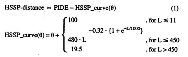
The simplest way to measure sequence similarity is percentage pairwise sequence identity (PIDE), that is, the percentage of residues identical between two proteins divided by residues aligned (not counting gaps). The second measure that we used was given by the statistical expectation values as reported by BLAST (E-VAL, note, we typically report the logarithm of this value in our figures). The third scoring scheme we used was the distance from the HSSP curve (Sander and Schneider 1991; Rost 1999):
 |
(1) |
in which L was the length of the alignment between two proteins, PIDE the percentage of pairwise identical residues, and HSSP_ curve(θ) the revised HSSP threshold for the level θ. As described above, we chose θ = 4 to reduce the bias. However, to compile distances, we chose the threshold of θ ( 0.
Modifications to optimise detection of homologs.
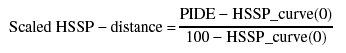
We introduced two modifications of the standard HSSP-distance (Eq. 1). (1) Perpendicular HSSP distance; to calculate the perpendicular HSSP distance (Eq. 1), percentage sequence identity and alignment length have to be measured in comparable units. This was done by first identifying approximate saturation points (slope 0 or ∞) on the HSSP curve. Using these saturation points, we rescaled the length of alignment axis (L in Eq. 1), and expressed it in terms of percent identity. For a given alignment, the normal to the rescaled HSSP curve was first identified. The length of the normal gave the perpendicular HSSP distance. We experimented with various rescaling constants. Finally, a rescaling constant of 0.26 for the length of alignment was observed to provide the best results. (2) Scaled HSSP distance; two proteins with 100% identical residues (PIDE = 100) over an alignment length of 25 residues have an HSSP distance of only 33. However, we observed very few false positives even over relatively short fragments for very similar pairs (Fig. 5 ▶). This suggested that better identification of homologs might be possible by using a relative distance from the curve. The scaled HSSP distance was defined as:
 |
(2) |
in which PIDE was the percentage pairwise sequence identity, and the HSSP_curve was as defined in Eq. 1 (with a threshold of 0).
Definitions of accuracy and coverage.
We used the following definitions to measure accuracy/specificity:
 |
(3) |
 |
with the thresholds given by either (1) percentage pairwise sequence identity, (2) BLAST expectations values, (3) the distance from the HSSP curve (Eq. 1), (4) the Scaled HSSP distance (Eq. 2), or (5) the Perpendicular HSSP distance. We considered all pairs as true that were experimentally found in the same subcellular compartment. In analogy, we used the following definitions for coverage/sensitivity:
 |
(4) |
 |
The accuracy of prediction was measured using the ratios:
 |
(5) |
 |
Note that pL and oL measure two different aspects of prediction methods, in particular, oL reflects how many of the known proteins are correctly predicted, whereas pL reflects how many of the predicted proteins are correctly predicted. For example, a method that strongly overpredicts (like SignalP) yields a high oL and a low pL (Table 3).
Prediction methods.
The prediction accuracy of three publicly available subcellular localization predictors was evaluated using the sequence-unique test set (Table 1). The three predictors were as follows: (1) NNPSL, neural network-based tool for predicting subcellular localization on the basis of amino acid composition (Reinhardt and Hubbard 1998) ; (2) SubLoc, a support vector machine-based tool for predicting subcellular localization on the basis of amino acid composition (Hua and Sun 2001); and (3) TargetP, neural network-based tool for large-scale subcellular localization prediction on the basis of amino-terminal sequence information (Emanuelsson et al. 2000). All methods were run with default parameter settings.
Annotating localization based on homology.
All proteins belonging to five entirely sequenced eukaryotic proteomes (Homo sapiens, Mus musculus, Drosophila melanogaster, Caenorhabditis elegans, and Arabidopsis thaliana) and all proteins in the SWISS-PROT database were aligned by pairwise BLAST to our data set of proteins with experimentally known localization (Table 1). We measure sequence similarity by the scaled HSSP distance, and considered only alignment pairs above the conservation threshold (scaled HSSP distance = 4). We estimated the accuracy of the annotation transfer by homology using the curves that were obtained for the different localizations (Fig. 4C ▶). We annotated localization on the basis of the known localization of the closest homolog. We annotated only those proteins for which localization could be inferred with >70% accuracy (Table 2).
Acknowledgments
We thank Dariusz Przybylski, Kazimierz Wrzeszczynski, and Trevor Siggers (all Columbia University) for crucial discussions; Jinfeng Liu (Columbia University) for providing genome data and computer assistance; and Cinque Soto and Yanay Ofran (both Columbia University) for helpful comments on the manuscript. We thank Astrid Reinhardt (Baylor College of Medicine, Texas), Tim Hubbard (Sanger Centre, Hinxton), Sujun Hua (Tsinghua University), Zhirong Hun (Tsinghua University), Olof Emanuelsson (Stockholm University), Henrik Nielsen (Technical University of Denmark), Søren Brunak (Technical University of Denmark), and Gunnar von Heijne (Stockholm University) for access to their prediction methods. The work of R.N. and B.R. was supported by the grants 1-P50-GM62413-01 and RO1-GM63029-01 from the National Institute of Health. Last, but not least, thanks to all those who deposit their experimental data in public databases, and to those who maintain these databases.
The publication costs of this article were defrayed in part by payment of page charges. This article must therefore be hereby marked "advertisement" in accordance with 18 USC section 1734 solely to indicate this fact.
Abbreviations
EC, Enzyme commission classification of enzymes
E-val, BLAST expectation value
GO, GeneOntology, that is, functional classification of proteins
HSSP, database of protein structure-sequence alignments
HSSP-distance, distance from function relating sequence identity and alignment length (Eq. 1)
PIDE, percentage pairwise sequence identity
proteome, we refer to the set of all proteins in an entirely sequenced organism as the proteome of that organism
LALI, length of sequence alignments
SWISS-PROT, curated database of protein sequences
Article and publication are at http://www.proteinscience.org/cgi/doi/10.1110/ps.0207402.
References
- Abagyan, R.A. and Batalov, S. 1997. Do aligned sequences share the same fold? J. Mol. Biol. 273 355–368. [DOI] [PubMed] [Google Scholar]
- Alexandrov, N.N. and Soloveyev, V.V. 1998. Statistical significance of ungapped sequence alignments. In HICCS `98: Pacific symposium on biocomputing `98. (eds. R.B. Altman, A.K. Dunker, L. Hunter, and T.E. Klein), pp. 463–472. World Scientific, Maui, Hawaii. [PubMed]
- Altschul, S.F. 1993. A protein alignment scoring system sensitive at all evolutionary distances. J. Mol. Evol. 36 290–300. [DOI] [PubMed] [Google Scholar]
- Altschul, S.F. and Gish, W. 1996. Local alignment statistics. Meth. Enzymol. 266 460–480. [DOI] [PubMed] [Google Scholar]
- Altschul, S.F., Gish, W., Miller, W., Myers, E.W., and Lipman, D.J. 1990. Basic local alignment search tool. J. Mol. Biol. 215 403–410. [DOI] [PubMed] [Google Scholar]
- Altschul, S., Madden, T., Shaffer, A., Zhang, J., Zhang, Z., Miller, W., and Lipman, D. 1997. Gapped Blast and PSI-Blast: A new generation of protein database search programs. Nucleic Acids Res. 25 3389–3402. [DOI] [PMC free article] [PubMed] [Google Scholar]
- Andrade, M.A., O'Donoghue, S.I., and Rost, B. 1998. Adaptation of protein surfaces to subcellular location. J. Mol. Biol. 276 517–525. [DOI] [PubMed] [Google Scholar]
- Andrade, M.A., Brown, N.P., Leroy, C., Hoersch, S., de Daruvar, A., Reich, C., Franchini, A., Tamames, J., Valencia, A., Ouzounis, C., et al. 1999. Automated genome sequence analysis and annotation. Bioinformatics 15 391–412. [DOI] [PubMed] [Google Scholar]
- Ashburner, M. and Drysdale, R. 1994. FlyBase–the Drosophila genetic database. Development 120 2077–2079. [DOI] [PubMed] [Google Scholar]
- Bairoch, A. and Apweiler, R. 2000. The SWISS-PROT protein sequence database and its supplement TrEMBL in 2000. Nucleic Acids Res. 28 45–48. [DOI] [PMC free article] [PubMed] [Google Scholar]
- Blake, J.D. and Cohen, F.E. 2001. Pairwise sequence alignment below the twilight zone. J. Mol. Biol. 307 721–735. [DOI] [PubMed] [Google Scholar]
- Bork, P. and Koonin, E.V. 1998. Predicting functions from protein sequences—where are the bottlenecks? Nat. Genet. 18 313–318. [DOI] [PubMed] [Google Scholar]
- Brenner, S.E., Chothia, C., and Hubbard, T.J.P. 1998. Assessing sequence comparison methods with reliable structurally identified distant evolutionary relationships. Proc. Natl. Acad. Sci. 95 6073–6078. [DOI] [PMC free article] [PubMed] [Google Scholar]
- Bruce, B.D. 2000. Chloroplast transit peptides: Structure, function and evolution. Trends Cell Biol. 10 440–447. [DOI] [PubMed] [Google Scholar]
- Casari, G., Andrade, M.A., Bork, P., Boyle, J., Daruvar, A., Ouzounis, C., Schneider, R., Tamames, J., Valencia, A., and Sander, C. 1995. Challenging times for bioinformatics. Nature 376 647–648. [DOI] [PubMed] [Google Scholar]
- Chothia, C. and Lesk, A.M. 1986. The relation between the divergence of sequence and structure in proteins. EMBO J. 5 823–826. [DOI] [PMC free article] [PubMed] [Google Scholar]
- Claros, M.G., Brunak, S., and von Heijne, G. 1997. Prediction of N-terminal protein sorting signals. Curr. Opin. Struct. Biol. 7 394–398. [DOI] [PubMed] [Google Scholar]
- Cokol, M., Nair, R., and Rost, B. 2000. Finding nuclear localisation signals. EMBO Reports 1 411–415. [DOI] [PMC free article] [PubMed] [Google Scholar]
- Devos, D. and Valencia, A. 2000. Practical limits of function prediction. Proteins 41 98–107. [PubMed] [Google Scholar]
- ———. 2001. Intrinsic errors in genome annotation. Trends Genet. 17 429–431. [DOI] [PubMed] [Google Scholar]
- Doolittle, R.F. 1986. Of URFs and ORFs: A primer on how to analyze derived amino acid sequences. University Science Books, Mill Valley, CA.
- Drawid, A. and Gerstein, M. 2000. A Bayesian system integrating expression data with sequence patterns for localizing proteins: Comprehensive application to the yeast genome. J. Mol. Biol. 301 1059–1075. [DOI] [PubMed] [Google Scholar]
- Eisenhaber, F. and Bork, P. 1998. Wanted: Subcellular localization of proteins based on sequence. Trends Cell Biol. 8 169–170. [DOI] [PubMed] [Google Scholar]
- Emanuelsson, O., Nielsen, H., Brunak, S., and von Heijne, G. 2000. Predicting subcellular localization of proteins based on their N-terminal amino acid sequence. J. Mol. Biol. 300 1005–1016. [DOI] [PubMed] [Google Scholar]
- Faust, M. and Montenarh, M. 2000. Subcellular localization of protein kinase CK2. A key to its function? Cell Tissue Res. 301 329–340. [DOI] [PubMed] [Google Scholar]
- Ferrigno, P. and Silver, P.A. 1999. Regulated nuclear localization of stress-responsive factors: How the nuclear trafficking of protein kinases and transcription factors contributes to cell survival. Oncogene 18 6129–6134. [DOI] [PubMed] [Google Scholar]
- Hegyi, H. and Gerstein, M. 1999. The relationship between protein structure and function: A comprehensive survey with application to the yeast genome. J. Mol. Biol. 288 147–164. [DOI] [PubMed] [Google Scholar]
- Hobohm, U., Scharf, M., Schneider, R., and Sander, C. 1992. Selection of representative protein data sets. Protein Sci. 1 409–417. [DOI] [PMC free article] [PubMed] [Google Scholar]
- Hua, S. and Sun, Z. 2001. Support vector machine approach for protein subcellular localization prediction. Bioinformatics 17 721–728. [DOI] [PubMed] [Google Scholar]
- Jaroszewski, L., Rychlewski, L., and Godzik, A. 2000. Improving the quality of twilight-zone alignments. Protein Sci. 9 1487–1496. [DOI] [PMC free article] [PubMed] [Google Scholar]
- Karp, P.D. 1998. What we do not know about sequence analysis and sequence databases. Bioinformatics 14 753–754. [DOI] [PubMed] [Google Scholar]
- Koonin, E.V. 2000. Bridging the gap between sequence and function. Trends Genet. 16 16. [DOI] [PubMed] [Google Scholar]
- Koonin, E.V., Bork, P., and Sander, C. 1994. Yeast chromosome III: New gene functions. EMBO J. 13 493–503. [DOI] [PMC free article] [PubMed] [Google Scholar]
- Lewis, S., Ashburner, M., and Reese, M.G. 2000. Annotating eukaryote genomes. Curr. Opin. Struct. Biol. 10 349–354. [DOI] [PubMed] [Google Scholar]
- Liscovitch, M., Czarny, M., Fiucci, G., Lavie, Y., and Tang, X. 1999. Localization and possible functions of phospholipase D isozymes. Biochim. Biophys. Acta 1439 245–263. [DOI] [PubMed] [Google Scholar]
- Liu, J. and Rost, B. 2001. Comparing function and structure between entire proteomes. Protein Sci. 10 1970–1979. [DOI] [PMC free article] [PubMed] [Google Scholar]
- Mattaj, I.W. and Englmeier, L. 1998. Nucleocytoplasmic transport: The soluble phase. Annu. Rev. Biochem. 67 265–306. [DOI] [PubMed] [Google Scholar]
- Murzin, A.G. 1998. How far divergent evolution goes in proteins. Curr. Opin. Struct. Biol. 8 380–387. [DOI] [PubMed] [Google Scholar]
- Nakai, K. 2001. Prediction of in vivo fates of proteins in the era of genomics and proteomics. J. Struct. Biol. 134 103–116. [DOI] [PubMed] [Google Scholar]
- Nielsen, H., Engelbrecht, J., Brunak, S., and von Heijne, G. 1997. Identification of prokaryotic and eukaryotic signal peptides and prediction of their cleavage sites. Protein Eng. 10 1–6. [DOI] [PubMed] [Google Scholar]
- Nielsen, H., Brunak, S., and von Heijne, G. 1999. Machine learning approaches for the prediction of signal peptides and other protein sorting signals. Protein Eng. 12 3–9. [DOI] [PubMed] [Google Scholar]
- Ouzounis, C., Casari, G., Sander, C., Tamames, J., and Valencia, A. 1996. Computational comparisons of model genomes. Trends Biotechnol. 14 280–285. [DOI] [PubMed] [Google Scholar]
- Park, J., Karplus, K., Barrett, C., Hughey, R., Haussler, D., Hubbard, T., and Chothia, C. 1998. Sequence comparisons using multiple sequences detect three times as many remote homologues as pairwise methods. J. Mol. Biol. 284 1201–1210. [DOI] [PubMed] [Google Scholar]
- Pawlowski, K., Jaroszewski, L., Rychlewski, L., and Godzik, A. 2000. Sensitive sequence comparison as protein function predictor. Pac. Symp. Biocomput. 8 42–53. [DOI] [PubMed] [Google Scholar]
- Pearce, D.A. 2000. Localization and processing of CLN3, the protein associated to Batten disease: Where is it and what does it do? J. Neurosci. Res. 59 19–23. [PubMed] [Google Scholar]
- Pearson, W.R. 1995. Comparison of methods for searching protein sequence databases. Protein Sci. 4 1145–1160. [DOI] [PMC free article] [PubMed] [Google Scholar]
- Przybylski, D. and Rost, B. 2002. Alignments grow, secondary structure prediction improves. Proteins 46 195–205. [DOI] [PubMed] [Google Scholar]
- Reich, J.G. and Meiske, W. 1987. A simple statistical significance test of window scores in large dot matrices obtained from protein or nucleic acid sequences. Comput. Appl. Biosci. 3 25–30. [DOI] [PubMed] [Google Scholar]
- Reinhardt, A. and Hubbard, T. 1998. Using neural networks for prediction of the subcellular location of proteins. Nucleic Acids Res. 26 2230–2235. [DOI] [PMC free article] [PubMed] [Google Scholar]
- Rost, B. 1997. Protein structures sustain evolutionary drift. Fold. Des. 2 S19–S24. [DOI] [PubMed] [Google Scholar]
- ———. 1998. Marrying structure and genomics. Structure 6 259–263. [DOI] [PubMed] [Google Scholar]
- ———. 1999. Twilight zone of protein sequence alignments. Protein Eng. 12 85–94. [DOI] [PubMed] [Google Scholar]
- ———. 2001. Protein secondary structure prediction continues to rise. J. Struct. Biol. 134 204–218. [DOI] [PubMed] [Google Scholar]
- ———. 2002. Enzyme function less conserved than anticipated. J. Mol. Biol. 318 595–608. [DOI] [PubMed] [Google Scholar]
- Rost, B and Eyrich, V. 2001. EVA: Large-scale analysis of secondary structure prediction. Proteins 45 S192–S199. [DOI] [PubMed] [Google Scholar]
- Rychlewski, L., Zhang, B., and Godzik, A. 1999. Functional insights from structural predictions: Analysis of the Escherichia coli genome. Protein Sci. 8 614–624. [DOI] [PMC free article] [PubMed] [Google Scholar]
- Sander, C. and Schneider, R. 1991. Database of homology-derived structures and the structural meaning of sequence alignment. Proteins 9 56–68. [DOI] [PubMed] [Google Scholar]
- Schatz, G. and Dobberstein, B. 1996. Common principles of protein translocation across membranes. Science 271 1519–1526. [DOI] [PubMed] [Google Scholar]
- Schneider, R., Casari, G., Antoine, d.D., Bremer, P., Schlenkrich, M., Mercille, R., Vollhardt, H., and Sander, C. 1997. GeneCrunch: Experiences on the SGI POWER CHALLENGE array with bioinformatics applications. In Supercomputer 1996: Anwendungen, Architekturen, Trends, pp. 109–119. K.G. Saur Verlag, Germany.
- Schwarz, E. and Neupert, W. 1994. Mitochondrial protein import: Mechanisms, components and energetics. Biochim. Biophys. Acta 1187 270–274. [DOI] [PubMed] [Google Scholar]
- Shah, I. and Hunter, L. 1997. Predicting enzyme function from sequence: Asystematic appraisal. In Fifth international conference on intelligent systems for molecular biology. (ed. T. Gaasterland, P. Karp, K. Karplus, C. Ouzounis, C. Sander, and A. Valencia), pp. 276–283. AAAI Press, Halkidiki, Greece. [PMC free article] [PubMed]
- Sirover, M.A. 1999. New insights into an old protein: The functional diversity of mammalian glyceraldehyde-3-phosphate dehydrogenase. Biochim. Biophys. Acta 1432 159–184. [DOI] [PubMed] [Google Scholar]
- Tamames, J., Ouzounis, C., Casari, G., Sander, C., and Valencia, A. 1998. EUCLID: Automatic classification of proteins in functional classes by their database annotations. Bioinformatics 14 542–543. [DOI] [PubMed] [Google Scholar]
- Teichmann, S., Park, J., and Chothia, C. 1998. Structural assignments to the Mycoplasma genitalium proteins show extensive gene duplication and domain rearrangement. Proc. Natl. Acad. Sci. 14658–14663. [DOI] [PMC free article] [PubMed]
- Teichmann, S.A., Chothia, C., and Gerstein, M. 1999. Advances in structural genomics. Curr. Opin. Struct. Biol. 9 390–399. [DOI] [PubMed] [Google Scholar]
- Thornton, J.M., Orengo, C.A., Todd, A.E., and Pearl, F.M. 1999. Protein folds, functions and evolution. J. Mol. Biol. 293 333–342. [DOI] [PubMed] [Google Scholar]
- Todd, A.E., Orengo, C.A., and Thornton, J.M. 2001. Evolution of function in protein superfamilies, from a structural perspective. J. Mol. Biol. 307 1113–1143. [DOI] [PubMed] [Google Scholar]
- Vitkup, D., Melamud, E., Moult, J., and Sander, C. 2001. Completeness in structural genomics. Nat Struct. Biol. 8 559–566. [DOI] [PubMed] [Google Scholar]
- Vogt, G., Etzold, T., and Argos, P. 1995. An assessment of amino acid exchange matrices in aligning protein sequences: The twilight zone revisited. J. Mol. Biol. 249 816–831. [DOI] [PubMed] [Google Scholar]
- Webb, E.C. 1992. Enzyme nomenclature 1992. Recommendations of the nomenclature committee of the International Union of Biochemistry and Molecular Biology., 1992 ed. Academic Press, New York.
- Wilson, C.A., Kreychman, J., and Gerstein, M. 2000. Assessing annotation transfer for genomics: Quantifying the relations between protein sequence, structure and function through traditional and probabilistic scores. J. Mol. Biol. 297 233–249. [DOI] [PubMed] [Google Scholar]
- Wood, T.C. and Pearson, W.R. 1999. Evolution of protein sequences and structures. J. Mol. Biol. 291 977–995. [DOI] [PubMed] [Google Scholar]
- Yang, A.S. and Honig, B. 2000a. An integrated approach to the analysis and modeling of protein sequences and structures. II. On the relationship between sequence and structural similarity for proteins that are not obviously related in sequence. J. Mol. Biol. 301 679–689. [DOI] [PubMed] [Google Scholar]
- ———. 2000b. An integrated approach to the analysis and modeling of protein sequences and structures. III. A comparative study of sequence conservation in protein structural families using multiple structural alignments. J. Mol. Biol. 301 691–711. [DOI] [PubMed] [Google Scholar]