Transmembrane helix predictions revisited

Abstract

Methods that predict membrane helices have become increasingly useful in the context of analyzing entire proteomes, as well as in everyday sequence analysis. Here, we analyzed 27 advanced and simple methods in detail. To resolve contradictions in previous works and to reevaluate transmembrane helix prediction algorithms, we introduced an analysis that distinguished between performance on redundancy-reduced high- and low-resolution data sets, established thresholds for significant differences in performance, and implemented both per-segment and per-residue analysis of membrane helix predictions. Although some of the advanced methods performed better than others, we showed in a thorough bootstrapping experiment based on various measures of accuracy that no method performed consistently best. In contrast, most simple hydrophobicity scale-based methods were significantly less accurate than any advanced method as they overpredicted membrane helices and confused membrane helices with hydrophobic regions outside of membranes. In contrast, the advanced methods usually distinguished correctly between membrane-helical and other proteins. Nonetheless, few methods reliably distinguished between signal peptides and membrane helices. We could not verify a significant difference in performance between eukaryotic and prokaryotic proteins. Surprisingly, we found that proteins with more than five helices were predicted at a significantly lower accuracy than proteins with five or fewer. The important implication is that structurally unsolved multispanning membrane proteins, which are often important drug targets, will remain problematic for transmembrane helix prediction algorithms. Overall, by establishing a standardized methodology for transmembrane helix prediction evaluation, we have resolved differences among previous works and presented novel trends that may impact the analysis of entire proteomes.

Helical membrane proteins challenge bioinformatics. Membrane proteins are crucial for survival. They constitute key components for cell–cell signaling, mediate the transport of ions and solutes across the membrane, and are crucial for recognition of self (Stack et al. 1995; Chapman et al. 1998; Le Borgne and Hoflack 1998; Chen and Schnell 1999; Hettema et al. 1999; Pahl 1999; Truscott and Pfanner 1999; Bauer et al. 2000; Ito 2000; Soltys and Gupta 2000; Thanassi and Hutltgren 2000). Furthermore, the pharmaceutical industry preferably targets membrane-bound receptors (Heusser and Jardieu 1997; Bettler et al. 1998; Moreau and Huber 1999; Saragovi and Gehring 2000; Sedlacek 2000). Despite their great biological and medical importance, we still have very little experimental information about their 3D structures: <1% of the proteins of known structure are membrane proteins. Fortunately, it is relatively easy to identify the location of membrane helices through low-resolution experiments. An expert-curated list of low-resolution experiments maintained by Steffen Möller and colleagues (Möller et al. 2000) considers information from C-terminal fusions with indicator proteins (McGovern et al. 1991; Hennessey and Broome-Smith 1993; Traxler et al. 1993; van Geest and Lolkema 2000) and from antibody-binding studies (Traxler et al. 1993; McGuigan 1994; Jermutus et al. 1998; Morris et al. 1998; Amstutz et al. 2001). Nevertheless, we only have low-resolution experimental information for <500 helical membrane proteins, and PDB (Berman et al. 2000) contains <50 sequence-unique protein chains with high-resolution helical membrane structures (Materials and Methods). These numbers contrast with the >7000 helical membrane proteins expected in humans alone (Wallin and von Heijne 1998; Krogh et al. 2001; Liu and Rost 2001). Thus, bioinformatics is challenged to help bridge the information gap between what we want and what we have.

Published estimates for membrane helix prediction questioned by recent analyses. Recently, a few groups have questioned the estimated levels of performance for membrane helix prediction methods. Möller, Croning, and Apweiler analyzed 14 prediction methods that did not use alignment information on a set of 188 proteins with experimentally known helices (Möller et al. 2000, 2001). They also applied the prediction methods to globular proteins and to signal peptides. The results indicated the following conclusions: (1) The best prediction method (TMHMM, transmembrane prediction using cyclic hidden Markov models) correctly predicts all membrane helices for 52%–69% of all proteins tested. (2) The best distinction between globular and membrane-helical proteins reaches levels of >97% for the globular proteins tested (TMHMM and SOSUI, hydrophobicity- and amphiphilicity-based transmembrane helix prediction). (3) On a set of 34 signal and transit peptide proteins, the best methods reached 98% (PHDhtm, profile-based neural network prediction of transmembrane helices) to 100% (ALOM2) accuracy in distinguishing these from membrane helices. (4) The best simple hydrophobicity index (KD, Kyte–Doolittle hydropathy index; Kyte and Doolittle 1982) correctly predicted all helices for 44% of all the proteins in a set for which HMMTOP (hidden Markov model predicting transmembrane helices; Tusnady and Simon 1998) reached only 43% accuracy. Another recent analysis was based on a set of 145 sequence-unique proteins (Ikeda et al. 2001). The researchers tested 10 prediction methods not using alignment information on their data set. In contrast to Möller et al., the investigators found that HMMTOP was not only much better than the KD hydrophobicity index, but that it was the most accurate prediction method, correctly predicting all membrane helices for ∼68% of all proteins. Averaging over all 10 methods, the authors found the resulting consensus prediction ∼10 percentage points more accurate than the best single method. The investigators also claimed that prediction accuracy is higher for prokaryotes than for eukaryotes. They speculated that they found different levels of accuracy than Möller et al. because they used different percentages of prokaryotic proteins in their data sets. Jayasinghe, Hristova, and White analyzed four prediction methods on two different sets of proteins with known membrane helix locations: (1) on 150 high-resolution structures from PDB, and (2) on 242 low-resolution proteins (Jayasinghe et al. 2001b). The researchers found that the results between the high- and low-resolution sets differed marginally and reported that the best methods (PHDhtm and HMMTOP) correctly predict >93%–97% of all helices. This group has also proposed a method based on a novel entropy-based hydrophobicity scale, namely, the Wimley–White scale (WW, Wimley–White hydrophobicity-scale-based method), which is claimed to correctly predict 99% of all membrane helices (Jayasinghe et al. 2001a). One major problem of hydrophobicity-based methods appears to be the poor distinction between membrane and globular proteins (Edelman 1993; Jones et al. 1994; Rost et al. 1995 Rost et al. 1996b; Jayasinghe et al. 2001a; Möller et al. 2001).

Problems with previous analyses. Previous analyses were limited in various ways. (1) Performance on high- and low-resolution data sets was distinguished by neither the Möller nor the Ikeda groups, although it seemed that performance differed between the two (Jayasinghe et al. 2001b). (2) The redundancy in data sets resulting from many copies of very similar proteins was not reduced by the Möller or Jayasinghe groups. However, such bias is known to create problems when estimating prediction methods (Rost and Sander 1993; Rost et al. 1995 Rost et al. 1996b; Rost 2002). (3) Neither Möller et al. nor Ikeda et al. tested any method based on alignment information, although such methods are known to be more accurate (Rost and Sander 1993; Persson and Argos 1994; Neuwald et al. 1995; Rost et al. 1995; Rost 1996; Johnson and Church 1999). (4) No group explored per-residue—along with per-segment—based measures for prediction accuracy. Instead, all groups focused on one particular definition of prediction accuracy; no two groups applied the same definition. (5) No group established levels for significant differences between methods. This makes it impossible to conclude whether or not differences between any two methods are relevant. In general, levels of significant differences typically depend on the data sets and the scores used (Eyrich et al. 2001; Rost and Eyrich 2001; Marti-Renom et al. 2002). (6) Only Möller and coworkers tested proteins with signal peptides; however, their analysis was restricted to a small set of 34 proteins with known signal peptides. (7) No group analyzed more than 14 prediction methods. (8) Generally, prediction accuracy differs significantly between proteins used to develop a method and proteins never seen by a method (Moult et al. 1995, 1997, 1999). For membrane proteins, this effect is very difficult to estimate because few high-resolution structures of membrane proteins are added over a course of a year. Although Möller et al. tried to estimate this effect by analyzing only proteins not used for developing a method, they did not rule out that the proteins tested in the category "not known to the method" were similar to proteins used for development. Surprisingly, Möller et al. found most methods to perform better on proteins not used for development. Given how prediction methods are developed, it is very unlikely that this result holds in general. Either the differences are not significant, or the data sets were not representative (or both).

To resolve these limitations and to standardize membrane helix prediction performance comparisons, we have presented an analysis that distinguished between performance on redundancy-reduced high- and low-resolution data sets, established thresholds for significant differences in performance by introducing a bootstrap experiment, and implemented both per-segment and per-residue analysis of membrane helix predictions. Additionally, we analyzed more methods (8 publicly available advanced prediction methods and 19 different hydrophobicity scales). In particular, we included alignment-based prediction methods. Furthermore, we tested membrane helix prediction methods on a large, representative set of 1418 unique signal peptides and 616 unique globular protein folds taken from SCOP (Lo Conte et al. 2002). Although we confirmed many previous findings, overall our results differed greatly in detail from previous publications.

Results

Accuracy in predicting membrane helices

Prediction methods not significantly less accurate than low-resolution experiments! We compared the membrane annotations for 13 proteins for which we had both low-resolution and high-resolution data available. Whereas ∼94%–96% of the helices agreed between the two experimental methods, for only 11 of the 13 proteins did all helices overlap between the two experimental methods (Table 1). Also, the two methods agreed on only 82% of all residue assignments (Table 1, Q₂, percentage of correctly predicted residues in two states: membrane helix and non-membrane helix). A detailed comparison of the percentage of identically assigned membrane-helical residues confirmed that for most cases, the differences arose from the longer segments observed in the high-resolution data (Q_2T^%obs < Q_2T^%prd, where Q_2T^%obs is the percentage of all observed TMH helix residues that are correctly predicted and Q_2T^%prd is the percentage of all predicted TMH helix residues that are correctly predicted). Assuming that the high-resolution data were correct, we can interpret the low-resolution data as an experimental prediction of transmembrane helices. Surprisingly, most prediction methods performed as well as the low-resolution experiments (Table 1). In fact, in terms of almost all measures for accuracy, we could find one method that numerically agreed more with the high-resolution data than the low-resolution experiment. However, given the small size of the data set, this statement ignored the error margins in the estimate for accuracy.

Table 1.

Accuracy of low-resolution experiments and predictions

	Per-segment accuracyb				Per-residue accuracyc
Methoda	Qok	Qhtm%obs	Qhtm%prd	TOPO	Q2	Q2T%obs	Q2T%prd	Q2N%obs	Q2N%prd
ERRORd	±16	±10	±10	±16	±6	±9	±9	±7	±7
LOW-RES	84	98	96	75	82	70	90	92	71
DAS	55	96	91		69e	46	91	94	58
HMMTOP2	93	99	99	62	78	67	88	85	66
PHDhtm08	83	98	98	64	79	74	77	85	82
PHDhtm07	85	98	98	64	79	74	77	85	82
PHDpsiHtm08	92	98	100	92	79	74	81	88	83
PRED-TMR	44	80	93		71	53	81	91	61
SOSUI	77	90	92		78	66	79	84	67
TMHMM1	77	89	92	53	80	66	82	87	68
TopPred2	78	96	99	61	76	65	87	83	65
WW	52	88	87		72	68	66	64	67

^a Methods: see abbreviations at begin of article.

^b Per-segment accuracy: Q_ok gives the percentage of proteins for which all TM helices are predicted correctly (eq. 4), Q_htm^%obs the percentage of all observed helices that are correctly predicted (eq. 2), Q_htm^%prd is the percentage of all predicted helices that are correctly predicted (eq. 3), TOPO the percentage of proteins for which the topology (orientation of helices) is correctly predicted (eq. 4, not: empty for methods that do not predict topology).

^c Per-residue accuracy: Q₂ is the percentage of correctly predicted residues in two-states: membrane helix/nonmembrane helix (eq. 6), Q_2T^%obs the percentage of all observed TMH helix residues that are correctly predicted (eq. 7), Q_2T^%prd the percentage of all predicted TMH helix residues that are correctly predicted (eq. 8), Q_2N^%obs the percentage of all observed non-TMH helix residues that are correctly predicted, and Q_2N^%prd the percentage of all predicted non-TMH helix residues that are correctly predicted.

Note of caution: this data set of 13 proteins was too small to rank the prediction methods in any way!

Data set: 13 high-resolution membrane helical proteins from PDB for which we found low-resolution experimental information in old versions of SWISS-PROT (labeled by LOW-RES). Note that the topology assessment was based on only 8 of the 13 proteins for which we had this information.

^d ERROR: The estimates for per-segment accuracy resulted from a bootstrap experiment with M = 100 and K = 6 (Fig. 5 ▶); the estimates for per-residue accuracy were obtained according to equation 11.

^e Numbers in italics: 2 standard deviations difference from baseline LOW-RES.

Simple hydrophobicity-based predictions were less accurate than advanced methods. Of the methods that only used hydrophobicity scales for prediction, none detected all membrane helices correctly for >70% of the high-resolution proteins (Table 2, Q_ok, percentage of proteins for which all TM helices are predicted correctly). However, most methods correctly identified >90% of all observed membrane helices (Table 2, Q_htm^%obs, percentage of all observed helices that are predicted correctly). In fact, measured by this score alone, most simple hydrophobicity-based methods appeared more accurate than many advanced prediction methods, but this success was achieved by overpredicting membrane helices (Table 2, Q_htm^%prd < Q_htm^%obs, where Q_htm^%prd is the percentage of all predicted helices that are predicted correctly). Encouragingly, >80% of the helices predicted by most methods were correct (Table 2, Q_htm^%prd). Unfortunately, the real problem with the simple methods was that they did not correctly predict the nonmembrane regions as apparent in levels of <70% correctly predicted residues (Table 2, Q₂). Note that we implemented all simple hydrophobicity scales by using the algorithm proposed by the White group (Jayasinghe et al. 2001a). To ensure that this optimized or at least did not penalize membrane protein prediction for some hydrophobicity scales, we also tested the thresholds suggested in the original publications for the GES (hydrophobicity property; Engelman et al. 1986^; Prabhakaran 1990) and KD scales (Kyte and Doolittle 1982). Interestingly, the originally proposed thresholds decreased prediction accuracy (Supplementary Table 1; available online at http://www.proteinscience.org).

Table 2.

Accuracy of prediction methods for high-resolution set

	Per-segment accuracy				Per-residue accuracy
Method	Qok	Qhtm%obs	Qhtm%prd	TOPO	Q2	Q2T%obs	Q2T%prd	Q2N%obs	Q2N%prd
ERROR	±10	±8	±10	±9	±3	±7	±8	±6	±6
DAS	79	99	96		72	48	94	96	62
HMMTOP2	83	99	99	61	80	69	89	88	71
PHDhtm08	64	77	76	54	78	76	82	84	79
PHDhtm07	69	83	81	50	78	76	82	84	79
PHDpsihtm08	84	99	98	66	80	76	83	86	80
PRED-TMR	61	84	90		76	58	85	94	66
SOSUI	71	88	86		75	66	74	80	69
TMHMM1	71	90	90	45	80	68	81	89	72
TopPred2	75	90	90	54	77	64	83	90	69
KD	65	94	89		67	79	66	52	67
GES	64	97	90		71	74	72	66	69
Ben-Tal	60	79	89		72	53	80	95	63
Eisenberg	58	95	89		69	77	68	57	68
Hopp-Woods	56	93	86		62	80	61	43	67
WW	54	95	91		71	71	72	67	67
Av-Cid	52	93	83		60	83	58	39	72
Roseman	52	94	83		58	83	58	34	66
Levitt	48	91	84		59	80	58	38	67
A-Cid	47	95	83		58	80	56	37	66
Heijne	45	93	82		61	85	58	34	64
Bull-Breese	45	92	82		55	85	55	27	66
Sweet	43	90	83		63	83	60	43	69
Radzicka	40	93	79		56	85	55	26	63
Nakashima	39	88	83		60	84	58	36	63
Fauchere	36	92	80		56	84	56	31	65
Lawson	33	86	79		55	84	54	27	63
EM	31	92	77		57	85	55	28	64
Wolfenden	28	43	62		62	28	56	97	56

Data set: 36 high-resolution membrane helical proteins from PDB; Note: We had reliable information about topology for only 35 of the 36 proteins.

Abbreviations as in Table 1.

Methods, hydrophobicity scales: see the abbreviations footnote at the beginning of the article for the advanced methods, and the list of hydrophobicity scales in the Materials and Methods section for the hydrophobicity scales. The advanced methods are sorted by alphabet, the simple hydrophobicity-based methods according to the Q_ok score.

ERROR: the estimates for per-segment accuracy resulted from a bootstrap experiment with M = 100 and K = 18 (Fig. 5 ▶); the estimates for per-residue accuracy were obtained according to equation 11.

Numbers in italics: two standard deviations below the numerically highest value in each column.

Note of caution: all methods are tested on the same set of proteins. However, the numbers are not from a cross-validation experiment, that is, some methods may have used some of the proteins for training. Generally, newer methods are more likely to be overestimated than older ones.

Most advanced predictions were correct. All advanced prediction methods correctly identified all helices for most high-resolution proteins (Table 2, Q_ok). In contrast, the only two methods we found to also accurately predict the orientation of the helices, that is, the topology, most often were TopPred2 (hydrophobicity-based membrane helix prediction) and HMMTOP2 (Table 2, TOPO, percentage of proteins for which the topology is correctly predicted). Note that HMMTOP2 was developed using all the 36 high-resolution chains for which we compiled the results. On the other hand, TopPred2 used only four of the 36 chains when it was developed. All methods tested correctly predicted >70% of the residues in either of the two states, TMH (T) and non-TMH (N, Table 2, Q₂). However, all methods significantly underpredicted residues in membrane helices (Table 2, Q_2T^%obs < Q_2T^%prd).

No single advanced method best by all scores. The set of 36 high-resolution proteins was small enough to require extreme caution in ranking methods based on numerical differences. When comparing pairwise ranks of the methods according to various scores, we found that no advanced method performed consistently best, and none consistently worst (Fig. 1 ▶). Interestingly, TMHMM1 and TopPred2 appeared to be the most representative methods in that the scores for these methods were most often indistinguishable from all other advanced methods in pairwise comparisons. In contrast, DAS appeared to be most unique in that it was often better and often worse than all other methods. Three methods were clearly more often worse than better: WW (5 times better/30 times worse), PRED-TMR (6/23), and SOSUI (7/26). Three methods were clearly more often better than worse: HMMTOP2 (21 times better/1 time worse), PHDpsihtm08 (divergent profile-based neural network prediction of transmembrane helices) (27/2), and PHDhtm08 (20/6).

Fig. 1.

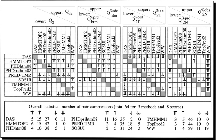
Pairwise comparison of methods. For all high-resolution results compiled in Table 2, we show the pairwise comparison for eight different scores and nine methods. Differences by more than one (two) standard error(s) are marked by one (two) arrow(s). Empty boxes indicate that the difference between the respective scores of the two methods is not significant. For example, DAS is two standard errors better than WW in terms of the number of correctly predicted proteins (Q_ok), whereas HMMTOP2 is two standard errors better than DAS in terms of the overall per-residue accuracy (Q₂). The lower table summarizes the respective counts of pair-comparisons for which a particular method is better or worse than the others. TopPred2 and TMHMM1 appear to be the most neutral method (44 and 46 times indistinguishable), whereas DAS seems the most unique method in that it is often better than the others and equally often worse. Note: only DAS, PHDhtm08, PHDpsihtm07, and TopPred2 did not use most of the proteins tested to optimize prediction accuracy; thus, the results for all the other methods are likely to be overestimates.

Performance on low-resolution data set: distinct differences. The low-resolution set was considerably larger (165 proteins) than the high-resolution set (36 chains). Nevertheless, we could still not find any method that performed consistently better than all the others (Table 3). Most methods reached better per-segment scores for the high- than for the low-resolution data. The opposite was the case for per-residue scores as they were consistently higher for the low-resolution proteins. Most surprising may be the significant differences between the two data sets in terms of the percentage of proteins for which all helices were correctly predicted for the old methods DAS and TopPred2 (Q_ok in Tables 2 and 3). Even more stunning was the extremely poor performance of most simple methods using only hydrophobicity scales for the prediction. Interestingly, for the hydrophobicity scales, the two newest ones (WW and Ben-Tal; hydrophobicity scale representing the free energy of transferring an amino acid from water into the center of the hydrocarbon region of a lipid bilayer) performed best overall on the data from low-resolution experiments.

Table 3.

Accuracy of prediction methods for low-resolution set

	Per-segment accuracy				Per-residue accuracy
Method	Qok	Qhtm%obs	Qhtm%prd	TOPO	Q2	Q2T%obs	Q2T%prd	Q2N%obs	Q2N%prd
ERROR	±9	±5	±5	±9	±2	±4	±4	±2	±2
DAS	39	93	81		86	65	85	97	84
HMMTOP2	66	94	93	79	90	85	83	91	91
PHDhtm08	57	86	86	68	87	83	75	90	94
PHDhtm07	56	85	86	72	87	83	75	90	94
PHDpsiHtm08	67	95	94	67	89	87	77	92	96
PRED-TMR	58	92	93		90	78	86	94	89
SOSUI	49	88	86		88	79	72	88	90
TMHMM1	72	91	92	85	90	83	80	91	92
TopPred2	48	84	79	59	88	74	71	93	89
Ben-Tal	35	79	90		87	67	83	95	85
Wolfenden	29	56	82		80	47	76	97	79
WW	27	90	75		81	83	59	77	89
GES	23	93	68		78	87	53	72	91
Eisenberg	20	90	63		72	89	47	63	91
KD	13	88	59		63	91	42	50	91
Heijne	11	89	55		51	91	35	33	89
Hopp-Woods	11	87	58		54	90	36	38	88
Sweet	11	87	59		58	88	38	44	87
Av-Cid	10	87	58		53	89	36	38	87
Roseman	9	89	56		48	91	34	30	88
Levitt	9	88	56		49	91	35	32	88
Nakashima	9	88	56		50	90	35	34	87
A-Cid	8	87	57		52	89	35	36	87
Lawson	8	86	57		43	89	32	24	83
Radzicka	6	87	56		41	91	32	21	85
Bull-Breese	6	86	56		40	91	32	20	83
EM	5	89	56		41	91	32	21	85
Fauchere	5	87	56		43	91	33	23	86

Data set: 165 low-resolution membrane helical proteins from SWISS-PROT (Möller et al. 2000).

Note: We had reliable information about topology only for 140 of the 165 proteins.

Abbreviations as in Table 2. The advanced methods are sorted by alphabet, the simple hydrophobicity-based methods according to the Q_ok score.

Numbers in italics: two standard deviations below the numerically highest value in each column.

Note of caution: all methods are tested on the same set of proteins. However, the numbers are not from a cross-validation experiment, that is, some methods may have used some of the proteins for training. Generally, newer methods are more likely to be overestimated than older ones. In particular, DAS, the PHD methods, and TopPred2 used only a small subset of these proteins for setting up the method, whereas HMMTOP2 used most.

Most errors were under- or overpredictions of one TMH. The good news was that all methods predicted the number of membrane helices correctly for most proteins (Fig. 2 ▶). However, this number differed significantly between the high- (71%) and the low-resolution data (56%). The majority of deviations were to predict one helix too few or one too many (68% for high; 64% for low-resolution, Fig. 2 ▶, center). Interestingly, the errors were rather symmetric for the low-resolution set, whereas they were substantially asymmetric for the high-resolution data. We could not find any significant correlation between the number of membrane helices and the errors of a particular method (data not shown). However, this may be largely owing to the few high-resolution structures in our data set.

Fig. 2.

Over- and underprediction of membrane helices. All methods (top panel): For all methods and all proteins in the high- and low-resolution sets, the difference between the number of membrane helices predicted and observed is shown. Although the two distributions appear rather similar, the higher symmetry in the low-resolution graph hid that the percentages with no difference were quite different: 71% for the high-resolution data and 56% for the low-resolution data. The inset (center) underlined the observation that the majority of errors were due to under- or overpredicting one helix.

Accuracy lower for proteins with more than five TMH’s. For proteins with five or fewer membrane helices, the average over all advanced methods exceeded 80% (Q_ok, eq. 4) for the high-resolution data and 60% for the low-resolution data (Fig. 3 ▶). However, prediction accuracy dropped significantly for proteins with more than five helices to values from 33%–36% (Fig. 3 ▶). Why are proteins with less than five TMH’s so different from proteins with more than six TMH’s? Answers to this question remain speculative.

Fig. 3.

Proteins with many helices predicted less accurately. We binned the results for all advanced methods according to the number of observed membrane helices such that the three classes contained similar numbers of proteins (X-axis). Accuracy (Y-axis) is measured in terms of the percentage of proteins for which all helices are correctly predicted (Q_ok). Both, for the high- and the low-resolution data, proteins with more than five membrane helices were predicted at significantly lower levels of accuracy.

Most proteins and most helices correctly predicted by one of the methods. None of the high-resolution helices has been consistently mispredicted by all programs. However, this may reflect that the more recent methods used all these proteins for training. In contrast, three transmembrane helices from three proteins of the low-resolution set were not identified by any of the methods: (1) The C4-dicarboxylate transport protein from Rhizobium meliloti (SWISS-PROT ID dcta_rhime; helix from residues 282–300, sequence ALPGLMNKMEKAGCKRSVV) has a relatively hydrophobic sequence, but it has a polar stretch of residues, NKMEK, in the middle of the helix. The gene fusion constructs were not always created with the reporter gene present in the predicted loop regions (Jording and Puhler 1993). In some cases, the reporter gene was present in the predicted membrane regions. This is a problem because it may alter the topological placement of the reporter gene with respect to the membrane. In addition, gene fusion constructs were not made for each loop region because reporter genes were introduced at random. Hence, each loop was not tested, which included loops for helix 282–300, for its topological placement. Hence, the experimental evidence for this membrane helix (282–300) was weak, at best. (2) The Haemolysin Secretion ATP-Binding Protein (HlyB) from Escherichia coli (hlyb_ecoli, residues 38–51, sequence GTGL GLTSWLLAAK) is an integral membrane protein. However, the particular membrane helix missed appears very short. The other seven membrane helices of HlyB are at least 20 residues long. However, some authors have claimed that membrane-spanning helices may be as short as 10 residues long (Lewis et al. 1990). The experimental evidence for hylb_ecoli had similar problems as that for dcta_rhime: The experimentalists found it difficult to identify membrane-spanning regions through predictions (Wang et al. 1991). This was caused by the high proportion of hydrophilic residues in the N-terminal portion of HlyB. Consequently, the authors did not know where to insert their reporter gene, which in this case was β-lactamase. Thus, they randomly inserted the reporter gene. Additionally, topological models identify the short stretch as loop (Wang et al. 1991; Gentschev and Goebel 1992). (3) Like all other problematic cases, the Mitochondrial brown fat uncoupling protein 1 from Rattus norvegicus (ucp1_rat, residues 178–194, sequence PNLMRNVIINCTELVTY) has transmembrane regions that contain many polar residues. For this protein, the experimentalists stated that their data did not suffice to strongly conclude that residues 178–194 are in a membrane helix (Miroux et al. 1993).

No significant difference in performance for prokaryotic and eukaryotic proteins. We compared the performance of each method for eukaryotic and prokaryotic proteins. Most methods did not consistently perform better for both the high- and low-resolution data (Table 4, ΔQ_ok). In fact, the trends differed greatly between both data sets, and for different measures of prediction accuracy. Whereas prokaryotic proteins were predicted more accurately in terms of per-segment measures for the high-resolution data sets, the opposite was the case for most methods when compared on the low-resolution set. Only four methods had a similar trend in Q_ok: PRED-TMR predicted eukaryotic proteins more accurately; SOSUI, TopPred2, and WW predicted prokaryotic proteins more accurately for both sets. However, none of the values exceeded two times the estimated error, that is, none was statistically very significant. All methods predicted topology (ΔTOPO) better for the prokaryotic proteins in the high-resolution set and for the eukaryotic proteins in the low-resolution set. When measuring prediction accuracy in terms of per-residue performance (ΔQ₂), we could not find any significant difference between prokaryotic and eukaryotic proteins; all methods did slightly better for eukaryotic proteins for both high- and low-resolution data. Nevertheless, because of the lack of consistent direction of the difference and the lack of statistical significance, our data did not support the previously published conclusion that either prokaryotic or eukaryotic proteins were predicted more accurately.

Table 4.

Difference between eukaryotic and prokaryotic membrane proteins

	Difference in accuracy eukaryotes vs. prokaryotes
	High-resolution			Low-resolution
Method	ΔQok	ΔTOPO	ΔQ2	ΔQok	ΔTOPO	ΔQ2
ERROR	±14	±12	±20	±18	±6	±18
DAS	4		4	−16		8
HMMTOP2	−9	−31	2	13	6	9
PHDhtm08	−24	−14	3	10	39	10
PHDhtm07	−11	−6	3	10	39	10
PHDpsiHtm08	−20	−32	3	13	32	8
PRED-TMR	5		5	11		7
SOSUI	−8		1	−18		5
TMHMM1	−20	−39	0	6	12	5
TopPred2	−12	−18	0	−12	−32	7
WW	−6		4	−12		5

Data set: eukaryotic proteins: 19 in high-resolution set, 73 in low-resolution set; prokaryotic proteins: 17 in high-resolution set, 87 in low-resolution set.

Accuracy: levels of accuracy given are the differences in the averages over all eukaryotic proteins minus the averages over all prokaryotic proteins.

Number in italics: values that are ± two standard deviations from a difference of 0.

Accuracy of distinguishing between membrane and other proteins

Few false positives: best methods found few membrane helices in globular proteins. Most advanced methods correctly distinguished between membrane and globular proteins (Table 5). The best methods confused between the two types of proteins for <4% of all globular proteins tested (Table 5). DAS had the highest error rate of the advanced methods (16% false positives), which was surprising given that DAS tended to underpredict residues in membrane helices. In contrast to the advanced methods, the simple methods distinguished only poorly between membrane and globular proteins. The two exceptions were the old scale from Wolfenden (hydration potential; Wolfenden et al. 1981) and the new one from Ben-Tal (Kessel and Ben-Tal 2002). The latter also predicted membrane proteins rather accurately (Tables 2 and 3). However, most methods found helices in >90% of all the globular proteins.

Table 5.

Confusion of membrane and globular proteins

		False negatives (%)
Method	False positives (%)	High-resolution	Low-resolution
ERROR	±2	±9	±3
SOSUI	1	8	4
TMHMM1	1	8	4
Wolfenden	2	39	13
PHDpsihtm	2	3	8
PHDhtm08	2	19	23
Ben-Tal	3	11	4
PHDhtm07	3	14	16
PRED-TMR	4	8	1
HMMTOP2	6	0	1
TopPred2	10	8	11
DAS	16	0	0
WW	32	0	0
GES	53	0	0
Eisenberg	66	0	0
KD	81	0	0
Sweet	84	0	0
Hopp-Woods	89	0	0
Nakashima	90	0	0
Heijne	92	0	0
Levitt	93	0	0
Roseman	95	0	0
A-Cid	95	0	0
Av-Cid	95	0	0
Lawson	98	0	0
FM	99	0	0
Fauchere	99	0	0
Bull-Breese	100	0	0
Radzicka	100	0	0

Data set: 616 high-resolution globular proteins from PDB (for false positives, i.e., the test whether or not the methods incorrectly predict membrane helices in globular proteins). The membrane sets are identical to those given in Table 2 (high-resolution) and Table 3 (low-resolution).

Methods are sorted by the accuracy in correctly rejecting globular protein (false positives).

Numbers in italics: two standard errors below the lowest confusion rate.

Few false negatives. Most methods find all membrane proteins. Although most hydrophobicity scales detected membrane helices in >90% of the globular proteins, they detected all membrane proteins as such. The exceptions were the two scales that were best in rejecting globular proteins: Wolfenden and Ben-Tal (Table 5). Similarly, PHDhtm08 misclassified only 2% of the globular proteins, but also missed ∼20% of the membrane proteins. The only methods that misclassified <10% of the globular proteins and overlooked <10% of the membrane proteins were: SOSUI, TMHMM1, PHDpsihtm, PRED-TMR, and HMMTOP2 (Table 5).

Signal peptides falsely predicted to be membrane helices by most methods. Even the advanced methods had high error rates for signal peptides (Table 6). In fact, one of the most accurate rejections of signal peptides was achieved by the simple method solely using the Wolfenden (Wolfenden et al. 1979) hydrophobicity scale (26% errors). Many of the false predictions were at the very beginning of the respective secreted proteins. Thus, we tested the following simple expert rule: delete all membrane helices predicted between 5 and 10 residues after an N-terminal methionine. For PHDpsihtm08, this reduced the falsely predicted signal peptides from 322 (23%) to 146 (10%). Encouragingly, when we applied the same rule to the set of membrane proteins, no helix was removed by this rule. For three out of the 1418 signal peptides, PHDpsihtm08 incorrectly predicted two transmembrane helices.

Table 6.

Incorrectly predicted membrane helices in signal peptides (false positives)

Method	Percentage of proteins with signal peptides
ERROR	±1
PHDpsihtm08	23
PHDhtm08	24
Wolfenden	26
TMHMM1	34
PHDhtm07	45
PRED-TMR	41
HMMTOP2	48
Ben-Tal	57
SOSUI	61
TopPred2	82
WW	90
DAS	97
GES	98
Eisenberg	99
KD	99
Sweet	99
Hopp-Woods	99
Nakashima	99
Heijne	99
Levitt	99
Roseman	99
A-Cid	99
Av-Cid	99
Lawson	99
EM	99
Fauchere	99
Bull-Breese	99
Radzicka	99

Data set: 1418 sequence unique signal peptides from http://www.cbs.dtu.dk/ftp/signalp/ collected by Nielsen and colleagues (Nielsen et al. 1996, 1997a,b).

Numbers in italics: two standard deviations below the lowest false-positive rate.

Discussion

Confirming previous analyses

Some methods correctly distinguish globular from helical membrane proteins. Previous analyses showed that simple hydrophobicity-based methods have problems distinguishing between helical transmembrane and globular proteins (Edelman 1993; Jones et al. 1994; Rost et al. 1995; Jayasinghe et al. 2001a; Möller et al. 2001). In general, we confirmed this finding (Table 5). However, the Wolfenden and the Ben-Tal scales were clearly exceptional in this respect. Both performed on a par with the best advanced methods that predict membrane helices in at most 3% of all globular proteins (Table 5). Interestingly, these levels of accuracy are similar to the performance of the same methods six years ago (Rost et al. 1996a,b). This finding confirms that the globular proteins added to PDB over the last decade are not radically different from the structures that we knew before (Rost and Sander 1993; Rost 2001). Möller and colleagues published significantly more pessimistic estimates for the confusion between globular and membrane proteins (Möller et al. 2001). Whereas our estimates were based entirely on proteins of known structure, those from Möller et al. were based on proteins of unknown structure. Thus, we see two possible reasons for the difference between the two estimates. (1) Proteins in PDB differ from proteins in SWISS-PROT in their average length by almost a factor of 2 because structural biologists often have to truncate the proteins to obtain high-resolution structures. We might argue that the truncated regions are more likely to be confused with membrane helices than the regions for which structure is determined. (2) Many of the proteins used by Möller and colleagues may, in fact, contain membrane helices or signal peptides (for which the error is higher, Table 6). We suspect that the truth lies somewhere between the two extremes. Hence, our estimates for the confusion between globular and membrane proteins may be slightly optimistic.

Most methods confuse signal peptides and membrane helices. Möller et al. tested prediction methods on 34 signal and target peptides. They found that most methods incorrectly predicted these regions to contain membrane helices. We tested all 27 methods on 1418 sequence-unique signal peptides. Our results confirmed the previously uncovered trends (Table 6). However, the larger set that we used revealed that TMHMM1, which is one of the best methods in this respect, confuses >30% of the signal peptides with membrane helices rather than <10% as previously estimated (Möller et al. 2001). Most simple methods based only on hydrophobicity scales confused >90% of all the signal peptides with membrane helices (exception: Wolfenden scale, Table 6). The good news was that the error could be reduced by experts who discard all membrane helices predicted closer than 10 residues to an N-terminal methionine. In this best-case scenario, PHDhtm and PHDpsihtm falsely predicted only ∼10% of the signal peptides as membrane helices. Possibly, combinations of membrane-optimized and signal-peptide-optimized programs could reduce this error rate.

Most methods identify most membrane helices. We confirmed (Ikeda et al. 2001; Jayasinghe et al. 2001b; Möller et al. 2001) that many methods correctly predict most membrane helices (Fig. 2 ▶). We also found the most common mistake to be the under- or overprediction of a single transmembrane helix. However, our results differed in detail from previous analyses (see below).

Resolving differences in previous analyses

Some methods are better; none is clearly best. Evaluations of membrane prediction methods are sometimes based on different definitions for performance accuracy. A particular example of the latter is to count a prediction of one long helix as correct although it stretches over two observed helices and thus misses the break in between the two. Another misleading standard procedure is to only report values covering one side of the coin, that is, only the values of correctly predicted as percentage of observed or vice versa. Here, we carefully evaluated all methods on identical data sets and compiled all reasonable scores for prediction accuracy. To simplify the complexity, we focused in our report on a relatively limited number of scores. Another problem with many previous analyses is that investigators have not estimated the error associated with a particular score. For example, from Table 1 we may conclude that HMMTOP2 is much better than TopPred2 when applying any measure for prediction accuracy. Although the numbers differed greatly, a thorough bootstrap experiment revealed that the performance of the two methods was indeed indistinguishable. We compared the methods in a pairwise manner for each score of the high-resolution data set (Fig. 1 ▶). Some methods appeared more accurate than others. However, no method(s) performed consistently better than all others by more than one standard error (Fig. 1 ▶). Our estimates of error margins explained the numerical differences found between three analyses (Ikeda et al. 2001; Jayasinghe et al. 2001b; Möller et al. 2001).

Simple hydrophobicity-based methods less accurate than advanced methods. Möller et al. (2001) suggested that simple hydrophobicity scale-based methods predict membrane helices almost as accurately as the best advanced methods. We could not confirm this proposition. In contrast, we found that the best advanced methods were significantly more accurate than the best hydrophobicity-scale based methods, both in terms of per-segment and per-residue accuracy (Tables 2 and 3). The only possible exception may be the per-residue performance of the Ben-Tal scale for the low-resolution data (Table 3). However, we did confirm that, because of overprediction, a few hydrophobicity-scale-based methods identify the observed membrane helices at a level of accuracy similar to that of advanced methods in Q_htm^%obs in Tables 2 and 3. Jayasinghe et al. found that the WW hydrophobicity scale-based method that they introduced outperformed even the best advanced methods ("We find that [the] WW scale … identifies TM helices of membrane proteins with an accuracy greater than 99%"; Jayasinghe et al. 2001a). We could also not confirm this finding, no matter which definition of prediction accuracy we compared. Nevertheless, the major problem with simple hydrophobicity-based methods is their failure on globular proteins (Table 5) and signal peptides (Table 6). In fact, the error of hydrophobicity scales depends on the length of the protein. For example, the high-resolution chains had an average length of ∼215 residues, whereas low-resolution proteins were, on average, ∼420 residues long. Although hydrophobicity scales correctly predicted all helices in 28%–65% of the short proteins (Table 2), they only detected 5%–29% for the long proteins (Table 3). In particular, the scale that performed best on the high-resolution set (KD) dropped in accuracy from 65% (high) to 13% (low), whereas the scale that performed most poorly on the short proteins in the high-resolution data (Wolfenden) became best for the long proteins in the low-resolution data. The Wolfenden scale also performed relatively well on globular proteins (Table 5) and on signal peptides (Table 6). The price for the lack of overprediction is a low accuracy in detecting membrane helices (underprediction). Overall, the most successful hydrophobicity scale appeared to be the Ben-Tal scale, which is based on the free energy of transferring an amino acid from water into the center of the hydrocarbon region of a lipid bilayer (Kessel and Ben-Tal 2002). It out-performed the Wolfenden scale for membrane proteins and for globular proteins, and it bested all other scales for the low-resolution set. Simple hydrophobicity scales obviously have tremendous importance for sequence analysis. However, to use them as the only criterion to predict membrane helices appears to be a bad idea.

Incorrect ranking by per-segment accuracy depends on definition of score. As discussed above, any attempt to rank prediction methods should account for the standard error in the estimated level of accuracy. A particular illustration of this finding is that different definitions of the accuracy in correctly predicting all helices (eq. 4) would slightly alter the ranks. For example, DAS scored worst among all advanced methods when an overlap of at least nine residues was required to consider a helix correctly predicted (definition introduced by Möller et al. 2001), but it appeared to be the third-best of all advanced methods when we applied the definition introduced by Ikeda et al. (2001) (see Supplementary Table 1; available online at http://www.proteinscience.org). When giving different ranks only for significant differences, this apparent contradiction was resolved. Most averages were relatively insensitive to whether we required an overlap of 3 or 9 residues between predicted and observed helix (Q_ok3 and Q_ok9 in Supplementary Table 1; available online at http://www.proteinscience.org). However, contrary to what has been claimed previously, some methods had lower averages when requiring nine overlapping residues. Similarly, for most methods the average scores did not change considerably when using the definition of Ikeda et al (Q_ok11Centre in Supplementary Table 1; available online at http://www.proteinscience.org). However, although the score was lower for most methods for which it differed from the other two, for a few it was actually higher. These were methods that tended to underpredict helices. Overall, the dependence of ranking on the definition of the score used underscored the need to standardize evaluations.

Similar prediction accuracy for prokaryotic and eukaryotic membrane proteins. Ikeda et al. (2001) found that prediction methods are consistently worse at predicting membrane proteins from eukaryotes than those from prokaryotes. We could not verify this finding. Both for the high- and for the low-resolution data sets, we found that some methods reached slightly higher levels on one than on the other (Table 4). However, the differences were not significant.

Novel findings

Low-resolution experiments not much more accurate than prediction methods. The low-resolution experiments differed substantially in their assignments of membrane helices from high-resolution experiments. In fact, for a small subset of 13 high-resolution chains, many prediction methods appeared to be as correct—or as incorrect—as previously deposited low-resolution experiments (Table 1). This problem was also reflected in the substantial differences between the numerical scores for some of the methods. For example, DAS, TopPred2, and the PHDhtm series used partial information about 9 of the 36 high-resolution chains for development. For these methods, the scores on the 27 cross-validated high-resolution chains were similar to those for the 36 high-resolution chains (data not shown). However, the per-segment scores for the low-resolution sets differed from those for the high-resolution sets (Tables 2 and 3, in particular Q_ok). There are two possible explanations for this: either the low-resolution set contains new motifs, or the low-resolution experiments over- or underassign many helices. Such errors could result in a particularly poor performance in terms of predicting all TM helices correctly. In fact, for the set of 13 proteins for which we had low- and high-resolution experiments, Q_ok was low (84%, Table 1) for the low-resolution experiments. Furthermore, the observation that DAS, TopPred2, and the PHDhtm series got higher per-residue scores on the low-resolution data than on the high-resolution data indicated that the low-resolution assignments might not reflect completely new membrane motifs. Thus, the estimate for these cross-validated methods may be correctly estimated by the high-resolution data set (Table 2).

Problems with topology assignments by low-resolution data. The topologies of two proteins were incorrectly assigned by the low-resolution experiments (Table 1). These two proteins were (1) PDB: 1EHK:B/SWISS-PROT: COX2_THETH; and (2) PDB: 1EUL:A/SWISS-PROT: ATA2_RABIT. (1) 1EHK:B has one membrane helix and the N terminus is in the periplasm. Thus, PDB annotates the topology IN. In contrast, SWISS-PROT (release 34) annotates COX2_THETH with topology OUT, despite experimental data indicating otherwise (Keightley et al. 1995). Note that the latest SWISS-PROT release still annotates COX2_THETH as OUT. (2) The second pair is more complicated: The old SWISS-PROT release 20 entry for ATCA_RABIT was annotated with 10 membrane helices with topology IN, whereas the PDB structure 1EUL:A has 10 membrane helices with topology OUT. In contrast, the latest SWISS-PROT release for ATA2_RABIT annotates 10 helices, but still assigns the topology as IN according to antibody studies (Moller et al. 1997). However, this experimentally determined topology may be incorrect because of nonspecific antibodies for the N-terminus epitope. Indeed, the experimentalists noted that the antibody against the N terminus was only immunoreactive to the 1–243 N-terminal fragment rather than specific to the N-terminal 12 residues. At the same time, they argued that this antiserum can correctly locate the epitope for residues 1–12 (Juul et al. 1995). They suggested that the N terminus is cytoplasmic, but for other cytosolic loops, the authors observed enhanced antibody reactivities. Additionally, the N terminus may be OUT because after solubilization with C₁₂E₆, proteolysis did not drastically increase reactivity of antiserum 1–12. Furthermore, antisera to epitopes on all loop regions of ATA2_RABIT were not tested. Therefore, it would be useful to acquire information of the location of the other loops in ATA2_RABIT to verify the topological orientation of this protein.

All prediction methods missed only helices with weak experimental evidence. None of the helices in the high-resolution set and only three in the low-resolution set were missed by all advanced methods. As described above (in Results), the experiments done for these three proteins were not fully convincing in terms of the assignments of transmembrane helices and topology. This observation suggests implementing a consensus prediction of membrane helices. The potential success of such an approach has been initially tried out by a couple of authors (Promponas et al. 1999; Ikeda et al. 2001). However, these two initial attempts have focused only on advanced methods. Although advanced methods are more accurate than simple hydrophobicity-based methods, they tend to underpredict transmembrane helices, especially for high-resolution structures (Table 2). Advanced methods could thus serve as a specificity filter for a consensus method. Using both advanced and simple methods could help to verify low-resolution experimental results from proteolysis and gene fusion.

Not all membrane proteins identified. The only advanced method that predicted all known helical membrane proteins to contain at least one helix was DAS (Table 5, false negatives). However, the flip-side of the same coin was that DAS also performed poorly on globular proteins (Table 5, false positives). The other extreme was PHDhtm, based on conventional pairwise alignments that performed well in rejecting globular proteins while also missing almost one-fifth of the membrane proteins with the default parameters. Obviously, there is a tradeoff between predicting too many globular as membrane proteins, and too many membrane as globular proteins. Possibly the best compromise was achieved by SOSUI and TMHMM, which missed 6% of the membrane proteins while incorrectly predicting membrane helices in ∼1% of all globular proteins. PHDhtm based on PSI-BLAST profiles (PHDpsihtm) reached a similar compromise: 8% of the membrane proteins were missed, and 2% of all globular proteins were mispredicted. Nevertheless, the problem of missing membrane proteins underlines once again that we need better methods that correctly distinguish between globular and membrane proteins.

Dependence of prediction accuracy on number of helices. We did not find any significant difference in the performance between proteins with one and many membrane proteins. In contrast, proteins with ≤5 membrane helices (≤5) were predicted more accurately than proteins with more (>6, Fig. 2B ▶). Although we could label the difference as significant, we failed to come up with any reasonable explanation for this finding. Readers may speculate that the numerical differences we observe between 6TM and 7TM proteins could be explained by the overabundance of transporters with buried charged residues. However, the number of proteins in each category was too small to validate such a fine-grained distinction.

Conclusion

We also overestimated the performance. Although we spent considerable effort on comparing prediction methods, our comparisons suffered from one crucial problem: We do not have cross-validation data available for all methods. In fact, the only methods for which we had cross-validated results were DAS, PHDhtm, PHDpsihtm, TopPred2, and most of the simple methods using only hydrophobicity scales. Although the overall scores for the advanced methods did not differ substantially between the sets of 27 cross-validated and 36-non-cross-validated high-resolution chains (data not shown), they did differ markedly between the nine chains used for development and the 27 cross-validated chains. This seemingly contradictory result is explained by the simple fact that most high-resolution proteins were not used in the development of these methods. In contrast, the newer prediction methods PRED-TMR, SOSUI, TMHMM, and WW used most and HMMTOP2 used all of the high-resolution chains for development. In fact, we observed two trends: (1) Newer methods were slightly better than older ones (HMMTOP2 was clearly more accurate than HMMTOP1 when tested on a small subset of the data); and (2) methods based on alignments were superior to those based on single sequences; in fact, when switching from using MaxHom (dynamic programming algorithm for conservation weight-based multiple sequence alignment) alignments against SWISS-PROT as input to PHDhtm to using PSI-BLAST alignments against all known sequences (BIG—nonidentical merger of SWISS-PROT and TrEMBL and PDB—and PHDpsiHtm), prediction accuracy increased considerably.

Most methods get most membrane helices, but the type of membrane protein is often wrong. The most common mistake was the under- or overprediction of one transmembrane helix. This appears encouraging in terms of prediction methods, in general. However, membrane predictions are very important in the context of analyzing entire proteomes because the number and orientation of the helices typically reveal aspects about function. In fact, only the very best methods predict all helices and the topology more often correctly than not. We may rightfully argue that present methods are still not good enough. Because both the number of helices and their orientation can easily be altered by engineering (Nilsson and von Heijne 1998; Ota et al. 1998; Monne et al. 1999a,b), the task at hand is, however, not an easy one. These experiments along with our analysis of the conservation of transmembrane helices strongly argue against the view that the number and orientation of membrane helices constitute a "solid reality written into the sequence." Rather, single residue exchanges can alter these macroscopic features. Thus, correct predictions require a precision typically not achieved. Perhaps present methods have reached the maximum possible level of accuracy and the chapter of simply predicting the location and orientation of membrane proteins is closed. With the recent high-resolution structures challenging common assumptions and our present analysis highlighting the number of urgent problems with prediction methods, we strongly doubt this. Therefore, we challenge that the issues elucidated in this investigation have reopened the field rather than closed it.

Materials and methods

Data sets

High-resolution data sets for membrane proteins. We started with a total set of 105 chains from helical membrane proteins for which a high-resolution structure was deposited in PDB (Berman et al. 2000). We identified these as helical membrane proteins according to the excellent up-to-date collection of membrane proteins at http://blanco.biomol.uci.edu (Jayasinghe et al. 2001b).

Low-resolution data sets for membrane proteins. We used an expert-curated set of 165 helical membrane proteins that was collected by Stefan Möller and colleagues (Möller et al. 2000). For all these proteins, good low-resolution experimental evidence about localization was available. For the comparison between high-resolution and low-resolution data, we used the annotations we found about transmembrane helix location in old SWISS-PROT versions released prior to the publication of the high-resolution structures.

High-resolution data set for globular proteins. The EVA server (Eyrich et al. 2001) continuously maintains a sequence-unique subset of PDB proteins. We used the version from July 2001 with 1852 representative protein chains. From that set we first removed all membrane proteins. Then we removed all proteins that were similar to one representative in a SCOP superfamily (Murzin et al. 1995; Lo Conte et al. 2000). Representatives were taken to be the longest proteins in the respective superfamily. This procedure yielded a final set of 616 globular protein chains.

Data set of proteins with known signal peptides. Henrik Nielsen and colleagues at the CBS in Copenhagen keep an up-to-date list of experimentally known signal peptides at their Web site (http://www.cbs.dtu.dk/ftp/signalp/readme). This group also spent considerable effort at defining thresholds for what constitutes redundancy in sets of signal peptides (Nielsen et al. 1996, 1997a). We downloaded a set of 1418 sequence-unique signal peptides from a total list of 2845.

Sequence-unique subsets reduce bias. Many of the proteins for which we have information about TM regions are similar to one another. If we want to analyze prediction methods or simple features such as TM length, this bias is problematic. To reduce the bias from the set of enzymes of known function, we have to first generate all-against-all alignments that capture the bias existing in that set. Then, we have to choose the maximal subset that fulfils the constraint that no pair in that subset is sequence-similar. Technically, we accomplished this objective in the following way. First, a pairwise BLAST (Altschul and Gish 1996) aligned all membrane proteins against each other. Second, the resulting pairs were filtered applying the HSSP-threshold (value θ = 0, below) such that all remaining pairs were likely to have similar structures. Third, the resulting families were sorted by number of members and length. Fourth, all pairs were clustered with a simple greedy algorithm starting with the largest and longest families (Hobohm et al. 1992). Note that the threshold chosen roughly translated to "no pair with more than 33% sequence identity over more than 100 residues aligned." In particular, we used the following formula to compile the distance DIST from the HSSP-curve HSSP_PIDE (Rost 1999):

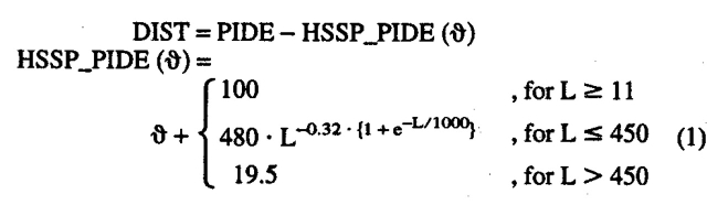(1)

where PIDE is the percentage pairwise sequence identity (ignoring gaps and insertions). This procedure yielded 36 proteins in the high-resolution set, and 165 proteins in the low-resolution set.

Programs tested

Building multiple alignments. Two different alignment schemes were explored: (1) the dynamic programming method MaxHom (Sander and Schneider 1991), and (2) a profile-based PSI-BLAST (Altschul et al. 1997). The particular protocol for finding similarities with PSI-BLAST applied the usual precautions to avoid drift and pollution (Jones 1999; Przybylski and Rost 2002). Searches were restricted to three iterations, and the iteration parameter (H-value) to 10⁻¹⁰ was set. The search databases were SWISS-PROT (Bairoch and Apweiler 2000) and BIG (SWISS-PROT [Bairoch and Apweiler 2000] + TrEMBL [Bairoch and Apweiler 2000] + PDB [Berman et al. 2000]). To explore the conservation of membrane helices, we filtered all MaxHom alignments according to various distances θ (eq. 1).

Advanced prediction methods. We referred to prediction methods as advanced when they implement more than simple hydrophobicity scales. We tested the following programs: DAS, HMMTOP (version 2), PHDhtm, PHDpsihtm, PRED-TMR, SOSUI, TMHMM (version 2), and TopPred2. TopPred2 averages the GES-scale of hydrophobicity (Engelman et al. 1986) using a trapezoid window (von Heijne 1992; Sipos and von Heijne 1993). PHDhtm combines a neural network using evolutionary information with a dynamic programming optimization of the final prediction (Rost et al. 1995,Rost et al. 1996b). DAS optimizes the use of hydrophobicity plots (Cserzö et al. 1997). SOSUI (Hirokawa et al. 1998) uses a combination of hydrophobicity and amphiphilicity preferences to predict membrane helices. TMHMM is the most advanced, and seemingly most accurate, present method to predict membrane helices (Sonnhammer et al. 1998). It embeds a number of statistical preferences and rules into a hidden Markov model to optimize the prediction of the localization of membrane helices and their orientation (note: similar concepts are used for HMMTOP; Tusnady and Simon 1998). PRED-TMR uses a standard hydrophobicity analysis with emphasis on detecting the ends and beginnings of membrane helices (Pasquier et al. 1999).

Simple methods exclusively based on hydrophobicity scales. We also implemented our in-house prediction methods that simply used various hydrophobicity scales for prediction. In particular, we tested the following scales: A-Cid, normalized hydrophobicity scale for α-proteins (Cid et al. 1992); Av-Cid, normalized average hydrophobicity scale (Cid et al. 1992); Ben-Tal, Hydrophobicity scale representing free energy of transfer of an amino acid from water into the center of the hydrocarbon region of a model lipid bilayer (Kessel and Ben-Tal 2002); Bull-Breese, Bull-Breese hydrophobicity scale (Bull 1974); Eisenberg, normalized consensus hydrophobicity scale (Eisenberg et al. 1984); EM, Solvation free energy (Eisenberg and McLachlan 1986); Fauchere, hydrophobic parameter π from the partitioning of N-acetyl-amino-acid amides (Fauchere and Pliska 1983); GES, hydrophobicity property (Engelman et al. 1986; Prabhakaran 1990); Heijne, transfer free energy to lipophilic phase (von Heijne and Blomberg 1979); Hopp-Woods, Hopp-Woods hydrophilicity value (Hopp and Woods 1981); KD, Kyte–Doolittle hydropathy index (Kyte and Doolittle 1982); Lawson, transfer free energy (Lawson et al. 1984); Levitt, hydrophobic parameter (Levitt 1976); Nakashima, normalized composition of membrane proteins (Nakashima et al. 1990); Radzicka, transfer free energy from 1-octanol to water (Radzicka and Wolfenden 1988); Roseman, solvation-corrected side-chain hydropathy (Roseman 1988); Sweet, optimal matching hydrophobicity (Sweet and Eisenberg 1983); Wolfenden, hydration potential (Wolfenden et al. 1981); and WW, Wimley–White scale (Jayasinghe et al. 2001a). Replacing the WW scale with each of the above-mentioned hydrophobicity indices, we used the WW algorithm to evaluate the predictive performance of each index.

Measuring accuracy

Measuring per-segment accuracy. The ultimate goal of prediction methods obviously is to correctly predict all residues. Assume a protein with 10 membrane helices of 20 residues each; method A predicts 10 helices but gets the five residues at each end of each helix wrong, and method B misses four helices but gets the ends for the other six entirely right. Which method is better? Possibly, many readers would favor method A. This problem is captured in using two different scores measuring prediction accuracy in the field of globular secondary structure prediction: per-residue scores and per-segment scores (Rost and Sander 1993; Rost et al. 1994). Although globular secondary-structure segments are, on average, rather short (helices ∼10 residues, strands ∼5 residues), membrane helices are rather long. Consequently, the problem of evaluating the per-segment accuracy allows a more coarse-grained measure than required for globular secondary-structure prediction (Rost et al. 1994; Zemla et al. 1999). There are two separate issues to address when defining a helix to be predicted correctly. The first concerns counting the same helix twice. We used the simple concept of "correctly predicted segment" shown in Figure 4 ▶.

Fig. 4.

Correctly predicted segments. In this example, there are three observed and three predicted helices. Observed helix O1 is correctly predicted by P1 as they overlap. However, observed helix O2 is not correctly predicted because P1 already overlaps with O1. Hence, P1 cannot be used as a correct prediction for O2. Similarly, P2 is counted as correct only with respect to O3, whereas P3 is not since O3 was already predicted by P2.

In particular, the observed helix O2 is not correctly predicted, because P1 overlaps already with O1. Similarly, P2 is counted as correct with respect to O3, whereas P3 is not. The second issue concerns the minimal overlap required between the observed and predicted helix. If not stated otherwise, we required a minimal overlap of 3 residues, following the definitions previously used in many other publications (von Heijne 1992; Jones et al. 1994; Persson and Argos 1994; von Heijne 1994; Rost et al. 1995 Rost et al. 1996b; Persson and Argos 1996; Sonnhammer et al. 1998). Möller et al. (2001) used a similar procedure; however, they required an overlap of at least 9 rather than 3 residues. Other groups required a minimal overlap of 1 residue (e.g., Cserzö et al. 1997^; Tusnady and Simon 1998). Jayasinghe required an overlap of 9 (Jayasinghe et al. 2001b) and 3 (Jayasinghe et al. 2001a) residues; however, in both publications, they counted the same predicted helix twice, thus yielding 100% accuracy for the overlap between O1/P1 and O2/P2 in Figure 4 ▶. Yet another measure was introduced by Ikeda et al. (2001): Helices were considered as correctly predicted if the centers of the predicted and the observed helix overlapped by at least 11 residues. The different measures are illustrated in the following example for a prediction (T = transmembrane):

observed:

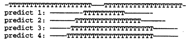
Jayasinghe et al. (2001a) evaluates prediction 1 as 0% accurate and 2–4 as 100% accurate (two helices correct); Jayasinghe et al. (2001b) give predictions 1 and 2 0% and 3 and 4 100%; Tusnady and Simon (1998) give 1–4 50% (one helix right, one not); Möller et al. (2001) give 1–2 0% and 3–4 50%; Ikeda et al. (2001) give 1–3 0% and 4 50%; the score that we refer to in this manuscript gives 1 0% and 2–4 50%. For comparison, we also provided a few other scores in the Supplementary Material (available online at http://www.proteinscience.org; note that we, however, did not count helices twice in any of those definitions).

With this concept, we can compile the percentage of correctly predicted transmembrane helices:

(2)

where Q_htm^%obs estimates the likelihood that an actual membrane helix is correctly predicted. Although this score can also be compiled for a single protein, it would be misleading to compile the score for each protein in a data set and then to average over all proteins. Rather, the number should be compiled by pooling all membrane helices from an entire data set. Overpredictions are measured by the corresponding score:

(3)

where Q_htm^%prd estimates the likelihood that a predicted TM is correctly predicted. These two scores are merged into a score that describes for which percentage of the proteins all TM segments are correctly predicted:

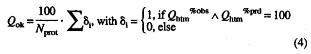(4)

Thus, Q_ok becomes 100 if and only if for all proteins in the set both Q_htm^%obs and Q_htm^%prd reach 100%. Finally, we need to evaluate the accuracy of predicting the topology correctly:

(5)

Measuring per-residue accuracy. Although the per-segment scores capture most of what experts would intuitively consider as important features of TMH prediction methods, we also need to monitor a number of per-residue scores that evaluate how accurately particular residues are predicted. In particular, the example of P2 and P3 in Figure 4 ▶ would yield 0 for all per-segment scores, although the predictions somehow capture important information. The simplest per-residue score is the two-state per-residue accuracy Q₂, which measures the percentage of residues predicted correctly in either of the two states T (membrane helix) or N (not membrane):

(6)

Typically, most residues in membrane proteins are in globular regions (Liu and Rost 2001). Thus, nonmembrane residues tend to dominate Q₂. This problem can be overcome by simply measuring the percentage of residues correctly predicted in membrane segments:

(7)

Similar to the per-segment scores, overpredictions can be captured by the corresponding score:

(8)

Q_2N^%obs and Q_2N^%prd are the corresponding percentages for nonmembrane residues. Finally, we monitored the Matthews correlation index (Matthews 1975) that attempts to capture both over- and underprediction of residues in transmembrane helices by one single score. This index is defined as:

(9)

where p_T is the number of residues correctly predicted as membrane helix (TMH), n_T is the number of residues correctly predicted as non-TMH, and u_T and o_T are the number of residues under- and overpredicted, respectively.

Estimating error for per-residue accuracy: standard error. For globular proteins, prediction accuracy varies considerably between different proteins (Rost et al. 1993; Rost 1996). The corresponding distributions can be approximated by Gaussian distributions. Thus, we can estimate the standard error of score Q by the simple rule-of-thumb:

(10)

where σ is the standard deviation for score Q based on a data set of N_prot-large proteins. This set has to be sufficiently large to actually observe a normal distribution. Assuming that we only have a much smaller data set of N_prot-set proteins, we can then still approximate the standard error by using the standard deviation compiled over the large data set. Whereas this concept is easy to apply to evaluations of globular prediction methods (Eyrich et al. 2001; Rost and Eyrich 2001), for the situation of membrane proteins, we simply do not have a sufficient number of high-resolution structures to once and for all estimate σ. There is no clean solution to this problem. Here, we used the following approximation:

(11)

that is, we used the maximal possible standard error. Assume that σ = 20 for a set of 13 proteins, σ = 10 for a set of 36 proteins, and σ = 15 for a set of 27 proteins. Then we used σ = 20 for the first, and σ = 15 for the other two.

Estimating error for per-segment accuracy: bootstrap experiment. The above concept to estimate the error in evaluating performance is not applicable for the per-segment scores, because these are not distributed normally. To illustrate the problem for the topology prediction: scores can be 1 (correct topology) or 0 (incorrect) for one protein. The score TOPO (eq. 5) averages over all proteins, hence provides one single final value, rather than a distribution. One way to still estimate the error in such a situation is the bootstrap experiment (Diaconis and Efron 1983; Efron et al. 1996). The procedure is the following (Fig. 5 ▶): (1) Assume we have a set of N = 36 proteins, each with correct or incorrect topology. (2) Choose a random subset of K < N proteins, and compile the average (TOPO) over these K proteins. (3) Repeat M times and estimate the error based on the resulting distribution of averages. In other words, the bootstrapping experiment attempts to estimate how sensitively a score depends on a particular data set chosen. Albeit often surprisingly powerful, bootstrapping is a more coarse-grained approximation. In particular, we used the following parameters to estimate errors for per-segment scores: M = 100 (100 random picks), and K = int(N/2); that is, for each random pick we chose half of the proteins available in the respective sets. Finally, we applied the same approximation as depicted in equation 11, that is, reported a rather conservative estimate for the error.

Fig. 5.

Procedure for estimating error using a bootstrap experiment. Given a data set with N items, one first defines K, which is the number of items one will select from the original data set, and M, which is the number of times one will choose a sample of size K. For instance, if the data set is of size 36, then one defines K < 36. Once K and M are defined, one selects a sample of size K and calculates the average value for the appropriate metric. Repeating this process M times will yield M average values. One can then compile the averaged value and standard deviation for these M average values.

Ranking methods. Given methods A and B evaluated on a set with N proteins, when can we conclude that the performance of A (Q(A)) is significantly better than that of B (Q(B))? The error estimates provide an answer to this question: We cannot distinguish between A and B if:

(12)

Thus, we can rank only if A and B differ by more than the error. For example, when a method correctly predicts 75% of the residues in a test set of 16 proteins with a standard deviation of 10%, a difference relative to another method that is smaller than 2.5% (i.e., ΔQ = 10/sqrt[16]) is not significant. Thus, we cannot distinguish between two methods that predict correctly 75% and 73% of all residues, respectively. We used this estimate to rank methods in the following way. Assume four methods have accuracy levels of A = 75, B = 73, C = 71, and D = 68. D can be distinguished from all other methods (ΔQ > 2.5 to all). Hence, it ranks last. C can be distinguished from A (ΔQ = 4 > 2.5). However, A cannot be distinguished from B (ΔQ = 2 < 2.5), and B cannot be distinguished from C (ΔQ = 2 < 2.5). This situation results in a dilemma that has four different possible solutions: (I) A, B, and C get the same rank, ascertaining that no two methods are ranked differently that cannot be distinguished. (II) A and B get rank 1, and C rank 2, ensuring that no two methods are ranked equally that can be distinguished. (III) A gets rank 1, B rank 2, and C rank 3, ignoring that we cannot distinguish between A and B, nor between B and C. (IV) Do not rank. None of these solutions is correct. Here, we applied solutions (IV) and (I). For the example given, solution (I) implied that A, B, and C ranked first; D ranked second. However, this simplification ignored another intrinsically insurmountable problem: What if method A is significantly better than method B in terms of Q₂ and significantly worse in terms of Q_ok? Occasionally, the following ad hoc solution is presented to such a problem: Rank all methods on all scores and compile averages over ranks (Tables 3 and 5).

Electronic supplemental material

All data sets and a few additional results are available through our Web site at: http://cubic.bioc.columbia.edu/papers/2002_htm_eval/data.

Abbreviations

• A-Cid, normalized hydrophobicity scale for α-proteins (Cid 1992)

• Av-Cid, normalized average hydrophobicity scale (Cid 1992)

• Ben-Tal, hydrophobicity scale representing the free energy of transferring an amino acid from water into the center of the hydrocarbon region of a lipid bilayer (Kessel and Ben-Tal 2002)

• BIG, nonidentical merger of SWISS-PROT (Bairoch and Apweiler 2000) and TrEMBL (Bairoch and Apweiler 2000) and PDB (Berman et al. 2000)

• BLAST, fast sequence alignment method (Altschul and Gish 1996)

• Bull-Breese, Bull-Breese hydrophobicity scale (Bull 1974)

• DSSP, program assigning secondary structure (Kabsch and Sander 1983)

• Eisenberg, normalized consensus hydrophobicity scale (Eisenberg et al. 1984)

• EM, Solvation free energy (Eisenberg and McLachlan 1986)

• EVA, server automatically evaluating structure prediction methods (Eyrich et al. 2001a,b)

• Fauchere, hydrophobic parameter π from the partitioning of N-acetyl-amino-acid amides (Fauchere and Pliska 1983)

• GES, hydrophobicity property (Engelman et al. 1986; Prabhakaran 1990)

• Heijne, transfer free energy to lipophilic phase (von Heijne and Blomberg 1979)

• HMM, hidden Markov model

• HMMTOP, hidden Markov model predicting transmembrane helices (Tusnady and Simon 1998)

• Hopp-Woods, Hopp-Woods hydrophilicity value (Hopp and Woods 1981)

• KD, Kyte–Doolittle hydropathy index (Kyte and Doolittle 1982)

• Lawson, transfer free energy (Lawson et al. 1984)

• Levitt, hydrophobic parameter (Levitt 1976)

• MaxHom, dynamic programming algorithm for conservation weight-based multiple sequence alignment (Sander and Schneider 1991)

• MEMSAT, dynamic-programming based prediction of transmembrane helices (Jones et al. 1994)

• META-PP, internet service allowing access to a variety of bioinformatics tools through one single interface (Eyrich and Rost 2000)

• Nakashima, normalized composition of membrane proteins (Nakashima et al. 1990)

• PDB, Protein Data Bank of experimentally determined 3D structures of proteins (Bernstein et al. 1977; Berman et al. 2000)

• PHDhtm, profile-based neural network prediction of transmembrane helices (Rost 1996; Rost et al. 1996b)

• PHDpsihtm, divergent profile (PSI-BLAST)-based neural network prediction 2002)

• PSI-BLAST, position-specific iterated database search (Altschul et al. 1997)

• Radzicka, transfer free energy from 1-octanol to water (Radzicka and Wolfenden 1988)

• Roseman, solvation-corrected side-chain hydropathy (Roseman 1988)

• SignalP, signal peptide prediction (Nielsen et al. 1997a)

• SOSUI, hydrophobicity- and amphiphilicity-based transmembrane helix prediction (Hirokawa et al. 1998)

• SPLIT, transmembrane helix prediction (Juretic et al. 1998)

• Sweet, optimal matching hydrophobicity (Sweet and Eisenberg 1983)

• SWISS-PROT, database of protein sequences (Bairoch and Apweiler 2000)

• TM, transmembrane

• TMAP, alignment-based prediction of transmembrane helices (Persson and Argos 1996)

• TMH, transmembrane helix

• TMHMM, transmembrane prediction using cyclic hidden Markov models (Sonnhammer et al. 1998; Krogh et al. 2001)

• TMpred, prediction of transmembrane helices (Hofmann and Stoffel 1993)

• TopPred2, hydrophobicity-based membrane helix prediction (von Heijne 1992; Cserzö et al. 1997)

• TrEMBL, translation of the EMBL-nucleotide database coding DNA to protein sequences (Bairoch and Apweiler 2000)

• Wolfenden, hydration potential (Wolfenden et al. 1981)

• WW, Wimley–White hydrophobicity scale-based method (Wimley et al. 1996a,b; White and Wimley 1999; White 2001).

References

- Altschul, S.F. and Gish, W. 1996. Local alignment statistics. Meth. Enzymol. 266 460–480. [DOI] [PubMed] [Google Scholar]
- Altschul, S., Madden, T., Shaffer, A., Zhang, J., Zhang, Z., Miller, W., and Lipman, D. 1997. Gapped BLAST and PSI-BLAST: A new generation of protein database search programs. Nucleic Acids Res. 25 3389–3402. [DOI] [PMC free article] [PubMed] [Google Scholar]
- Amstutz, P., Forrer, P., Zahnd, C., and Pluckthun, A. 2001. In vitro display technologies: Novel developments and applications. Curr. Opin. Biotechnol. 12 400–405. [DOI] [PubMed] [Google Scholar]
- Bairoch, A. and Apweiler, R. 2000. The SWISS-PROT protein sequence database and its supplement TrEMBL in 2000. Nucleic Acids Res. 28 45–48. [DOI] [PMC free article] [PubMed] [Google Scholar]
- Bauer, M.F., Hofmann, S., Neupert, W., and Brunner, M. 2000. Protein translocation into mitochondria: The role of TIM complexes. TICB 10 25–31. [DOI] [PubMed] [Google Scholar]
- Berman, H.M., Westbrook, J., Feng, Z., Gillliland, G., Bhat, T.N., Weissig, H., Shindyalov, I.N., and Bourne, P.E. 2000. The Protein Data Bank. Nucleic Acids Res. 28 235–242. [DOI] [PMC free article] [PubMed] [Google Scholar]
- Bernstein, F.C., Koetzle, T.F., Williams, G.J.B., Meyer, E.F., Brice, M.D., Rodgers, J.R., Kennard, O., Shimanouchi, T., and Tasumi, M. 1977. The Protein Data Bank: A computer based archival file for macromolecular structures. J. Mol. Biol. 112 535–542. [DOI] [PubMed] [Google Scholar]
- Bettler, B., Kaupmann, K., and Bowery, N. 1998. GABAB receptors: Drugs meet clones. Curr. Opin. Neurobiol. 8 345–350. [DOI] [PubMed] [Google Scholar]
- Bull, H.B.a.B. 1974. Surface tension of amino acid solutions: A hydrophobicity scale of the amino acid residues. Arch. Biochem. Biophys. 161 665–670. [DOI] [PubMed] [Google Scholar]
- Chapman, R., Sidrauski, C., and Walter, P. 1998. Intracellular signaling from the endoplasmic reticulum to the nucleus. Annu. Rev. Cell Dev. Biol. 14 459–485. [DOI] [PubMed] [Google Scholar]
- Chen, X. and Schnell, D.J. 1999. Protein import into chloroplasts. Trends Cell Biol. 9 222–227. [DOI] [PubMed] [Google Scholar]
- Cid, H., Bunster, M., Canales, M., and Gazitua, F. 1992. Hydrophobicity and structural classes in proteins. Prot. Engin. 5 373–375. [DOI] [PubMed] [Google Scholar]
- Cserzö, M., Wallin, E., Simon, I., von Heijne, G., and Elofsson, A. 1997. Prediction of transmembrane α-helices in prokaryotic membrane proteins: The dense alignment surface method. Prot. Engin. 10 673–676. [DOI] [PubMed] [Google Scholar]
- Diaconis, P. and Efron, B. 1983. Computer-intensive methods in statistics. Scient. Am. 248 96–108. [Google Scholar]
- Edelman, J. 1993. Quadratic minimization of predictors for protein secondary structure: Application to transmembrane α-helices. J. Mol. Biol. 232 165–191. [DOI] [PubMed] [Google Scholar]
- Efron, B., Halloran, E., and Holmes, S. 1996. Bootstrap confidence levels for phylogenetic trees. Proc. Natl. Acad. Sci. 93 13429–13434. [DOI] [PMC free article] [PubMed] [Google Scholar]
- Eisenberg, D. and McLachlan, A.D. 1986. Solvation energy in protein folding and binding. Nature 319 199–203. [DOI] [PubMed] [Google Scholar]
- Eisenberg, D., Weiss, R.M., and Terwilliger, T.C. 1984. The hydrophobic moment detects periodicity in protein hydrophobicity. Proc. Natl. Acad. Sci. 81 140–144. [DOI] [PMC free article] [PubMed] [Google Scholar]
- Engelman, D.M., Steitz, T.A., and Goldman, A. 1986. Identifying nonpolar transbilayer helices in amino acid sequences of membrane proteins. Annu. Rev. Biophys. Biophys. Chem. 15 321–353. [DOI] [PubMed] [Google Scholar]
- Eyrich, V. and Rost, B. 2000. The META-PredictProtein server. CUBIC, Columbia University, Department of Biochemistry and Molecular Biophysics. http://cubic.bioc.columbia.edu/predictprotein/submit_meta.html/.
- Eyrich, V., Martí-Renom, M.A., Przybylski, D., Fiser, A., Pazos, F., Valencia, A., Sali, A., and Rost, B. 2001. EVA: Continuous automatic evaluation of protein structure prediction servers. Bioinformatics 17 1242–1243. [DOI] [PubMed] [Google Scholar]
- Fauchere, J.L. and Pliska, V. 1983. Hydrophobic parameters π of amino-acid side chains from the partitioning of N-acetyl-amino-acid amides. Eur. J. Med. Chem. 18 369–375. [Google Scholar]
- Gentschev, I. and Goebel, W. 1992. Topological and functional studies on HlyB of Escherichia coli. Mol. Gen. Genet. 232 40–48. [DOI] [PubMed] [Google Scholar]
- Hennessey, E.S. and Broome-Smith, J.K. 1993. Gene-fusion techniques for determining membrane-protein topology. Curr. Opin. Str. Biol. 3 524–531. [Google Scholar]
- Hettema, E.H., Distel, B., and Tabak, H.F. 1999. Import of proteins into peroxisomes. Biochim. Biophys. Acta 1451 17–34. [DOI] [PubMed] [Google Scholar]
- Heusser, C. and Jardieu, P. 1997. Therapeutic potential of anti-IgE antibodies. Curr. Opin. Immunol. 9 805–813. [DOI] [PubMed] [Google Scholar]
- Hirokawa, T., Boon-Chieng, S., and Mitaku, S. 1998. SOSUI: Classification and secondary structure prediction system for membrane proteins. Bioinformatics 14 378–379. [DOI] [PubMed] [Google Scholar]
- Hobohm, U., Scharf, M., Schneider, R., and Sander, C. 1992. Selection of representative protein data sets. Protein Sci. 1 409–417. [DOI] [PMC free article] [PubMed] [Google Scholar]
- Hofmann, K. and Stoffel, W. 1993. TMBASE—A database of membrane spanning protein segments. Biol. Chem. Hoppe-Seyler 374 166. [Google Scholar]
- Hopp, T.P. and Woods, K.R. 1981. Prediction of protein antigenic determinants from amino acid sequences. Proc. Natl. Acad. Sci. 78 3824–3828. [DOI] [PMC free article] [PubMed] [Google Scholar]
- Ikeda, M., Arai, M., Lao, D.M., and Shimizu, T. 2001. Transmembrane topology prediction methods: A reassessment and improvement by a consensus method using a dataset of experimentally-characterized transmembrane topologies. In Silico Biol. 1: http://www.bioinfo.de/isb/2001/2002/0003/. [PubMed]
- Ito, A. 2000. Mitochondrial processing peptidase: Multiple-site recognition of precursor proteins. TICB 10 25–31. [DOI] [PubMed] [Google Scholar]
- Jayasinghe, S., Hristova, K., and White, S.H. 2001a. Energetics, stability, and prediction of transmembrane helices. J. Mol. Biol. 312 927–934. [DOI] [PubMed] [Google Scholar]
- ———. 2001b. MPtopo: A database of membrane protein topology. Protein Sci. 10 455–458. [DOI] [PMC free article] [PubMed] [Google Scholar]
- Jermutus, L., Ryabova, L.A., and Pluckthun, A. 1998. Recent advances in producing and selecting functional proteins by using cell-free translation. Curr. Opin. Biotechnol. 9 534–548. [DOI] [PubMed] [Google Scholar]
- Johnson, J.M. and Church, G.M. 1999. Alignment and structure prediction of divergent protein families: Periplasmic and outer membrane proteins of bacterial efflux pumps. J. Mol. Biol. 287 695–715. [DOI] [PubMed] [Google Scholar]
- Jones, D.T. 1999. Protein secondary structure prediction based on position-specific scoring matrices. J. Mol. Biol. 292 195–202. [DOI] [PubMed] [Google Scholar]
- Jones, D.T., Taylor, W.R., and Thornton, J.M. 1994. A model recognition approach to the prediction of all-helical membrane protein structure and topology. Biochem. 33 3038–3049. [DOI] [PubMed] [Google Scholar]
- Jording, D. and Puhler, A. 1993. The membrane topology of the Rhizobium meliloti C4-dicarboxylate permease (DctA) as derived from protein fusions with Escherichia coli K12 alkaline phosphatase (PhoA) and β-galactosidase (LacZ). Mol. Gen. Genet. 241 106–114. [DOI] [PubMed] [Google Scholar]
- Juretic, D., Zucic, D., Lucic, B., and Trinajstic, N. 1998. Preference functions for prediction of membrane-buried helices in integral membrane proteins. Comput. Chem. 22 279–294. [DOI] [PubMed] [Google Scholar]
- Juul, B., Turc, H., Durand, M., de Gracia, A., Denoroy, L., Moller, J., Champeil, P., and le Maire, M. 1995. Do transmembrane segments in proteolyzed sarcoplasmic reticulum Ca2+-ATPase retain their functional Ca2+ binding properties after removal of cytoplasmic fragments by proteinase K? J. Biol. Chem. 270 20123–20134. [DOI] [PubMed] [Google Scholar]
- Kabsch, W. and Sander, C. 1983. Dictionary of protein secondary structure: Pattern recognition of hydrogen bonded and geometrical features. Biopolymers 22 2577–2637. [DOI] [PubMed] [Google Scholar]
- Keightley, J., Zimmerman, B., Mather, M., Springer, P., Pastusztyn, A., Lawrence, D., and Fee, J. 1995. Molecular genetic and protein chemical characterization of the cytochrome ba3 from Thermus thermophilus HB8*. J. Biol. Chem. 270 20345–20358. [DOI] [PubMed] [Google Scholar]
- Kessel, A. and Ben-Tal, N. 2002. Free energy determinants of peptide association with lipid bilayers. In Peptide–lipid interactions (eds. S. Simon and T. McIntosh). Academic Press, San Diego (in press).
- Krogh, A., Larsson, B., von Heijne, G., and Sonnhammer, E.L. 2001. Predicting transmembrane protein topology with a hidden Markov model: Application to complete genomes. J. Mol. Biol. 305 567–580. [DOI] [PubMed] [Google Scholar]
- Kyte, J. and Doolittle, R.F. 1982. A simple method for displaying the hydropathic character of a protein. J. Mol. Biol. 157 105–132. [DOI] [PubMed] [Google Scholar]
- Lawson, E.Q., Sadler, A.J., Harmatz, D., Brandau, D.T., Micanovic, R., MacElroy, R.D., and Middaught, C.R. 1984. A simple experimental model for hydrophobic interactions in proteins. J. Biol. Chem. 259 2910–2912. [PubMed] [Google Scholar]
- Le Borgne, R. and Hoflack, B. 1998. Protein transport from the secretory to the endocytic pathway in mammalian cells. Biochim. Biophys. Acta 1404 195–209. [DOI] [PubMed] [Google Scholar]
- Levitt, M. 1976. A simplified representation of protein conformations for rapid simulation of protein folding. J. Mol. Biol. 104 59–107. [DOI] [PubMed] [Google Scholar]
- Lewis, M.J., Chang, J.A., and Simoni, R.D. 1990. A topological analysis of subunit A from Escherichia coli F1F0-ATP synthase predicts eight transmembrane segments. J. Biol. Chem. 265 10541–10550. [PubMed] [Google Scholar]
- Liu, J. and Rost, B. 2001. Comparing function and structure between entire proteomes. Protein Sci. 10 1970–1979. [DOI] [PMC free article] [PubMed] [Google Scholar]
- Lo Conte, L., Ailey, B., Hubbard, T.J., Brenner, S.E., Murzin, A.G., and Chothia, C. 2000. SCOP: A structural classification of proteins database. Nucleic Acids Res. 28 257–259. [DOI] [PMC free article] [PubMed] [Google Scholar]
- Lo Conte, L., Brenner, S.E., Hubbard, T.J., Chothia, C., and Murzin, A.G. 2002. SCOP database in 2002: Refinements accommodate structural genomics. Nucleic Acids Res. 30 264–267. [DOI] [PMC free article] [PubMed] [Google Scholar]
- Marti-Renom, M.A., Madhusudhan, M.S., Fiser, A., Rost, B., and Sali, A. 2002. Reliability of assessment of protein structure prediction methods. Structure 10 435–440. [DOI] [PubMed] [Google Scholar]
- Matthews, B.W. 1975. Comparison of the predicted and observed secondary structure of T4 phage lysozyme. Biochim. Biophys. Acta 405 442–451. [DOI] [PubMed] [Google Scholar]
- McGovern, K., Ehrmann, M., and Beckwith, J. 1991. Decoding signals for membrane proteins using alkaline phosphatase fusions. EMBO J. 10 2773–2782. [DOI] [PMC free article] [PubMed] [Google Scholar]
- McGuigan, J.E. 1994. Antibodies to complementary peptides as probes for receptors. Immunomethods 5 158–166. [DOI] [PubMed] [Google Scholar]
- Miroux, B., Frossard, V., Raimbault, S., Ricquier, D., and Bouillaud, F. 1993. The topology of the brown adipose tissue mitochondrial uncoupling protein determined with antibodies against its antigenic sites revealed by a library of fusion proteins. EMBO J. 12 3739–3745. [DOI] [PMC free article] [PubMed] [Google Scholar]
- Moller, J., Ning, G., Maunscbach, A., Fujimoto, K., Asai, K., Juul, B., Lee, T.-J., de Gracia, A., Falson, P., and le Maire, M. 1997. Probing of the membrane topology of sarcoplasmic reticulum Ca+2-ATPase with sequence-specific antibodies. J. Biol. Chem. 272 29015–29032. [DOI] [PubMed] [Google Scholar]
- Möller, S., Kriventseva, E.V., and Apweiler, R. 2000. A collection of well characterised integral membrane proteins. Bioinformatics 16 1159–1160. [DOI] [PubMed] [Google Scholar]
- Möller, S., Croning, D.R., and Apweiler, R. 2001. Evaluation of methods for the prediction of membrane spanning regions. Bioinformatics 17 646–653. [DOI] [PubMed] [Google Scholar]
- Monne, M., Gafvelin, G., Nilsson, R., and von Heijne, G. 1999a. N-Tail translocation in a eukaryotic polytopic membrane protein: Synergy between neighboring transmembrane segments. Eur. J. Biochem. 263 264–269. [DOI] [PubMed] [Google Scholar]
- Monne, M., Nilsson, I., Elofsson, A., and von Heijne, G. 1999b. Turns in transmembrane helices: Determination of the minimal length of a "helical hairpin" and derivation of a fine-grained turn propensity scale. J. Mol. Biol. 293 807–814. [DOI] [PubMed] [Google Scholar]
- Moreau, J.L. and Huber, G. 1999. Central adenosine A(2A) receptors: An overview. Brain Res. Brain Res. Rev. 31 65–82. [DOI] [PubMed] [Google Scholar]
- Morris, G.E., Sedgwick, S.G., Ellis, J.M., Pereboev, A., Chamberlain, J.S., and Nguyen thi, M. 1998. An epitope structure for the C-terminal domain of dystrophin and utrophin. Biochemistry 37 11117–11127. [DOI] [PubMed] [Google Scholar]
- Moult, J., Pedersen, J.T., Judson, R., and Fidelis, K. 1995. A large-scale experiment to assess protein structure prediction methods. Proteins 23 ii–iv. [DOI] [PubMed] [Google Scholar]
- Moult, J., Hubbard, T., Bryant, S.H., Fidelis, K., and Pedersen, J.T. 1997. Critical assessment of methods of protein structure prediction (CASP): Round II. Proteins Suppl 1 2–6. [PubMed] [Google Scholar]
- Moult, J., Hubbard, T., Fidelis, K., Pedersen, J.T. 1999. Critical assessment of methods of protein structure prediction (CASP): Round III. Proteins Suppl 3 2–6. [PubMed] [Google Scholar]
- Murzin, A.G., Brenner, S.E., Hubbard, T., and Chothia, C. 1995. SCOP: A structural classification of proteins database for the investigation of sequences and structures. J. Mol. Biol. 247 536–540. [DOI] [PubMed] [Google Scholar]
- Nakashima, H., Nishikawa, K., and Ooi, T. 1990. Distinct character in hydrophobicity of amino acid composition of mitochondrial proteins. Proteins 8 173–178. [DOI] [PubMed] [Google Scholar]
- Neuwald, A.F., Liu, J.S., and Lawrence, C.E. 1995. Gibbs motif sampling: Detection of bacterial outer membrane protein repeats. Protein Sci. 4 1618–1631. [DOI] [PMC free article] [PubMed] [Google Scholar]
- Nielsen, H., Engelbrecht, J., von Heijne, G., and Brunak, S. 1996. Defining a similarity threshold for a functional protein sequence pattern: The signal peptide cleavage site. Proteins 24 165–177. [DOI] [PubMed] [Google Scholar]
- Nielsen, H., Engelbrecht, J., Brunak, S., and von Heijne, G. 1997a. Identification of prokaryotic and eukaryotic signal peptides and prediction of their cleavage sites. Prot. Engin. 10 1–6. [DOI] [PubMed] [Google Scholar]
- ———. 1997b. A neural network method for identification of prokaryotic and eukaryotic signal peptides and prediction of their cleavage sites. Intl. J. Neural Sys. 8 581–599. [DOI] [PubMed] [Google Scholar]
- Nilsson, I. and von Heijne, G. 1998. Breaking the camel’s back: Proline-induced turns in a model transmembrane helix. J. Mol. Biol. 284 1185–1189. [DOI] [PubMed] [Google Scholar]
- Ota, K., Sakaguchi, M., von Heijne, G., Hamasaki, N., and Mihara, K. 1998. Forced transmembrane orientation of hydrophilic polypeptide segments in multispanning membrane proteins. Mol. Cell 2 495–503. [DOI] [PubMed] [Google Scholar]
- Pahl, H.L. 1999. Signal transduction from the endoplasmic reticulum to the cell nucleus. Physiol. Rev. 79 683–701. [DOI] [PubMed] [Google Scholar]
- Pasquier, C., Promponas, V.J., Palaios, G.A., Hamodrakas, J.S., and Hamodrakas, S.J. 1999. A novel method for predicting transmembrane segments in proteins based on a statistical analysis of the SwissProt database: The PRED-TMR algorithm. Prot. Engin. 12 381–385. [DOI] [PubMed] [Google Scholar]
- Persson, B. and Argos, P. 1994. Prediction of transmembrane segments in proteins utilising multiple sequence alignments. J. Mol. Biol. 237 182–192. [DOI] [PubMed] [Google Scholar]
- ———. 1996. Topology prediction of membrane proteins. Protein Sci. 5 363–371. [DOI] [PMC free article] [PubMed] [Google Scholar]
- Prabhakaran, M. 1990. The distribution of physical, chemical and conformational properties in signal and nascent peptides. Biochem. J. 269 691–696. [DOI] [PMC free article] [PubMed] [Google Scholar]
- Promponas, V.J., Palaios, G.A., Pasquier, C.M., Hamodrakas, J.S., and Hamodrakas, S.J. 1999. CoPreTHi: A Web tool which combines transmembrane protein segment prediction methods. In Silico Biol. 1 159–162. [PubMed] [Google Scholar]
- Przybylski, D. and Rost, B. 2002. Alignments grow, secondary structure prediction improves. Proteins 46 195–205. [DOI] [PubMed] [Google Scholar]
- Radzicka, A. and Wolfenden, R. 1988. Comparing the polarities of the amino acids: Side-chain distribution coefficients between the vapor phase, cyclohexane, 1-octanol, and neutral aqueous solution. Biochemistry 27 1664–1670. [Google Scholar]
- Roseman, M.A. 1988. Hydrophilicity of polar amino acid side-chains is markedly reduced by flanking peptide bonds. J. Mol. Biol. 200 513–522. [DOI] [PubMed] [Google Scholar]
- Rost, B. 1996. PHD: Predicting one-dimensional protein structure by profile based neural networks. Meth. Enzymol. 266 525–539. [DOI] [PubMed] [Google Scholar]
- ———. 1999. Twilight zone of protein sequence alignments. Prot. Engin. 12 85–94. [DOI] [PubMed] [Google Scholar]
- ———. 2001. Protein secondary structure prediction continues to rise. J. Struct. Biol. 134 204–218. [DOI] [PubMed] [Google Scholar]
- ———. 2002. Enzyme function less conserved than anticipated. J. Mol. Biol. 318 595–608. [DOI] [PubMed] [Google Scholar]
- Rost, B. and Eyrich, V. 2001. EVA: Large-scale analysis of secondary structure prediction. Proteins 45 Suppl 5: S192–S199. [DOI] [PubMed] [Google Scholar]
- Rost, B. and Sander, C. 1993. Prediction of protein secondary structure at better than 70% accuracy. J. Mol. Biol. 232 584–599. [DOI] [PubMed] [Google Scholar]
- Rost, B., Sander, C., and Schneider, R. 1993. Progress in protein structure prediction? TIBS 18 120–123. [DOI] [PubMed] [Google Scholar]
- ———. 1994. Redefining the goals of protein secondary structure prediction. J. Mol. Biol. 235 13–26. [DOI] [PubMed] [Google Scholar]
- Rost, B., Casadio, R., Fariselli, P., and Sander, C. 1995. Prediction of helical transmembrane segments at 95% accuracy. Protein Sci. 4 521–533. [DOI] [PMC free article] [PubMed] [Google Scholar]
- Rost, B., Casadio, R., and Fariselli, P. 1996a. Refining neural network predictions for helical transmembrane proteins by dynamic programming. In Fourth International Conference on Intelligent Systems for Molecular Biology (eds. D. States et al.), pp. 192–200. AAAI Press, St. Louis, MO. [PubMed]
- ———. 1996b. Topology prediction for helical transmembrane proteins at 86% accuracy. Protein Sci. 5 1704–1718. [DOI] [PMC free article] [PubMed] [Google Scholar]
- Sander, C. and Schneider, R. 1991. Database of homology-derived structures and the structural meaning of sequence alignment. Proteins 9 56–68. [DOI] [PubMed] [Google Scholar]
- Saragovi, H.U. and Gehring, K. 2000. Development of pharmacological agents for targeting neurotrophins and their receptors. Trends Pharmacol. Sci. 21 93–98. [DOI] [PubMed] [Google Scholar]
- Sedlacek, H.H. 2000. Kinase inhibitors in cancer therapy: A look ahead. Drugs 59 435–476. [DOI] [PubMed] [Google Scholar]
- Sipos, L. and von Heijne, G. 1993. Predicting the topology of eukaryotic membrane proteins. Eur. J. Biochem. 213 1333–1340. [DOI] [PubMed] [Google Scholar]
- Soltys, B.J. and Gupta, R.S. 2000. Mitochondrial proteins at unexpected cellular locations: Export of proteins from mitochondria from an evolutionary perspective. Intl. Rev. Cytol. 194 133–196. [DOI] [PubMed] [Google Scholar]
- Sonnhammer, E.L.L., von Heijne, G., and Krogh, A. 1998. A hidden Markov model for predicting transmembrane helices in protein sequences. In Sixth International Conference on Intelligent Systems for Molecular Biology (ISMB98) (eds. J. Glasgow et al.), pp. 175–182. AAAI Press, Montreal, Canada. [PubMed]
- Stack, J.H., Horazdovsky, B., and Emr, S.D. 1995. Receptor-mediated protein sorting to the vacuole in yeast: Roles for a protein kinase, a lipid kinase and GTP-binding proteins. Annu. Rev. Cell Dev. Biol. 11 1–33. [DOI] [PubMed] [Google Scholar]
- Sweet, R.M. and Eisenberg, D. 1983. Correlation of sequence hydrophobicities measures similarity in three-dimensional protein structure. J. Mol. Biol. 171 479–488. [DOI] [PubMed] [Google Scholar]
- Thanassi, D.G. and Hutltgren, S.J. 2000. Multiple pathways allow protein secretion across the bacterial outer membrane. Curr. Opin. Cell Biol. 12 420–430. [DOI] [PubMed] [Google Scholar]
- Traxler, B., Boyd, D., and Beckwith, J. 1993. The topological analysis of integral membrane proteins. J. Mem. Biol. 132 1–11. [DOI] [PubMed] [Google Scholar]
- Truscott, K.N. and Pfanner, N. 1999. Import of carrier proteins into mitochondria. Biol. Chem. 380 1151–1156. [DOI] [PubMed] [Google Scholar]
- Tusnady, G.E. and Simon, I. 1998. Principles governing amino acid composition of integral membrane proteins: Application to topology prediction. J. Mol. Biol. 283 489–506. [DOI] [PubMed] [Google Scholar]
- van Geest, M. and Lolkema, J.S. 2000. Membrane topology and insertion of membrane proteins: Search for topogenic signals. Microbiol. Mol. Biol. Rev. 64 13–33. [DOI] [PMC free article] [PubMed] [Google Scholar]
- von Heijne, G. 1992. Membrane protein structure prediction. J. Mol. Biol. 225 487–494. [DOI] [PubMed] [Google Scholar]
- ———. 1994. Membrane proteins: From sequence to structure. Annu. Rev. Biophys. Biomol. Struct. 23 167–192. [DOI] [PubMed] [Google Scholar]
- von Heijne, G. and Blomberg, C. 1979. Trans-membrane translocation of proteins: The direct transfer model. Eur. J. Biochem. 97 175–181. [DOI] [PubMed] [Google Scholar]
- Wallin, E. and von Heijne, G. 1998. Genome-wide analysis of integral membrane proteins from eubacterial, archaean, and eukaryotic organisms. Protein Sci. 7 1029–1038. [DOI] [PMC free article] [PubMed] [Google Scholar]
- Wang, R., Seror, S., Blight, M., Pratt, J., Broome-Smith, J., and Holland, I. 1991. Analysis of the membrane organization of an Escherichia coli protein translocator, HlyB, a member of a large family of prokaryote and eukaryote surface transport proteins. J. Mol. Biol. 217 441–454. [DOI] [PubMed] [Google Scholar]
- White, S. 2001. Membrane proteins of known structure. http://blanco.biomol.uci.edu/mp_assembly.html/.
- White, S.H. and Wimley, W.C. 1999. Membrane protein folding and stability: Physical principles. Annu. Rev. Biophys. Biomol. Struct. 28 319–365. [DOI] [PubMed] [Google Scholar]
- Wimley, W.C., Creamer, T.P., and White, S.H. 1996a. Solvation energies of amino acid side-chains and backbone in a family of host-guest pentapeptides. Biochemistry 35 5109–5124. [DOI] [PubMed] [Google Scholar]
- Wimley, W.C., Gawrisch, K., Creamer, T.P., and White, S.H. 1996b. A direct measurement of salt-bridge solvation energies using a peptide model system: Implications for protein stability. Proc. Natl. Acad. Sci. 93 2985–2990. [DOI] [PMC free article] [PubMed] [Google Scholar]
- Wolfenden, R.V., Cullis, P.M., and Southgate, C.C.F. 1979. Water, protein folding, and the genetic code. Science 206 575–577. [DOI] [PubMed] [Google Scholar]
- Wolfenden, R., Andersson, L., Cullis, P.M., and Southgate, C.C.B. 1981. Affinities of amino acid side chains for solvent water. Biochemistry 20 849–855. [DOI] [PubMed] [Google Scholar]
- Zemla, A., Venclovas, C., Fidelis, K., and Rost, B. 1999. A modified definition of SOV, a segment-based measure for protein secondary structure prediction assessment. Proteins 34 220–223. [DOI] [PubMed] [Google Scholar]