Scaffolding and validation of bacterial genome assemblies using optical restriction maps

Abstract

Motivation: New, high-throughput sequencing technologies have made it feasible to cheaply generate vast amounts of sequence information from a genome of interest. The computational reconstruction of the complete sequence of a genome is complicated by specific features of these new sequencing technologies, such as the short length of the sequencing reads and absence of mate-pair information. In this article we propose methods to overcome such limitations by incorporating information from optical restriction maps.

Results: We demonstrate the robustness of our methods to sequencing and assembly errors using extensive experiments on simulated datasets. We then present the results obtained by applying our algorithms to data generated from two bacterial genomes Yersinia aldovae and Yersinia kristensenii. The resulting assemblies contain a single scaffold covering a large fraction of the respective genomes, suggesting that the careful use of optical maps can provide a cost-effective framework for the assembly of genomes.

Availability: The tools described here are available as an open-source package at ftp://ftp.cbcb.umd.edu/pub/software/soma

Contact: mpop@umiacs.umd.edu

1 INTRODUCTION

Fast and cheap DNA sequencing technologies are an important prerequisite for accelerating research in many areas of medicine and biology, from personalized medicine and cancer research to the exploration of the multitude of bacteria inhabiting our world. The importance of genome sequencing in modern biological research is further highlighted by the announcement of an ‘X-prize’ for the first group that can successfully map the genomes of 100 humans in just 10 days.

In recent years, several companies have made advances towards this goal: the technology developed at 454 Life Sciences provides an order of magnitude higher throughput at a fraction of the cost of Sanger sequencing (Margulies et al., 2005), while the technology developed by Solexa/Illumina can generate an astounding 1 Gbp of DNA (one third of the human genome) during a single run of the sequencing machine, at a cost of only a few thousand dollars (www.solexa.com). In addition to 454 Life Sciences and Solexa, both of which are already being used in sequencing centers around the world, many other companies—Helicos, and Applied Biosystems, to name just a few—are participating in the race towards affordable high-throughput sequencing technologies.

The abundance of sequence information, however, does not necessarily make the task of deciphering a genome easier. Typically in a whole-genome shotgun (WGS) sequencing project, the sequence information consists of randomly sheared fragments whose order and orientation (which strand of DNA they come from) within the genome is not known. In order to minimize the chance that there exist regions of the genome not sampled by any of the fragments, sufficient fragments must be sequenced so as to oversample the genome several fold (a number referred to as the coverage of the genome). Piecing these sequences together (sequence assembly) is akin to solving a large puzzle, where multiple pieces are similar (repeats in the genome) and our eyesight is not perfect (errors in sequencing) (Pop, 2004).

In Sanger sequencing, the ‘traditional’ method for sequencing DNA, the sequenced fragments are relatively long (800–1000 bp) making it easy to disambiguate short repeats. In contrast, the sequences provided by emerging high-throughput technologies are generally of lower quality. For example, the 454 Life Sciences technology generates reads ∼250 bp in length, while Solexa generates even shorter reads, ∼35–40 bp. These datasets pose significant challenges to assembly algorithms and can, depending on the repeat complexity of the genome, lead to fragmented or incorrect assemblies. More importantly, however, these new technologies have significantly higher throughput than the Sanger method, leading to the need for the automated validation and scaffolding (determining relative placement of sequences) of the resulting assemblies. In this work, we address this issue by designing algorithms to automatically incorporate optical mapping information in the assembly process.

Optical mapping, a variant of restriction mapping, is one of multiple laboratory techniques aimed at mapping the location of specific landmarks along the DNA of an organism of interest. In both optical and restriction mapping, the landmarks correspond to the recognition sites for specific restriction enzymes. Restriction mapping involves cleaving a piece of unknown DNA using a restriction enzyme and then using gel-based methods to measure the range of fragment sizes represented in the sample. The spectrum of sizes obtained provides information about the structure of the unknown piece of DNA and can be viewed as a fingerprint of this sequence (Nathans and Smith, 1975). Optical mapping (Samad et al., 1995) extends this approach by providing, in addition to the set of fragment sizes, information about the order in which these fragments occur in the DNA (see Fig. 1 for a schematic representation of the map generation process). This information provides a genome-wide scaffold into which the sequence data can be placed [in a process somewhat akin to comparative assembly (Pop et al., 2004)]. Computational methods for performing this mapping are the focus of this article. Our work was motivated by the recent availability of accurate high-throughput methods for constructing optical maps (specifically the technology developed at Opgen, www.opgen.com) and its increased adoption as a valuable source of information (Latreille et al., 2007). Note that this technology allows an optical map to be constructed within as little as 24 h after receiving a DNA sample, a time-frame comparable to that needed for sequencing the sample with the 454 technology. Optical maps are, therefore, an attractive alternative to a 454-Sanger hybrid approach (Goldberg et al., 2006) as the construction of a paired-end library can take more than a week. Furthermore, since optical maps and paired-end data have complementary characteristics they can be used together when both data types are available. Optical maps provide a coarse, genome-wide scaffold, in contrast, with the typically fragmented scaffolds generated from paired-end data. The methods described in this article can be easily adapted to a hybrid optical map—paired-end approach by aligning entire paired-end scaffolds to the map instead of individual contigs.

Fig. 1.

The optical mapping process. To generate a whole-genome optical map, DNA is sheared into fragments that are stretched and fixed onto an optical chip and then digested using a restriction enzyme. The resulting pieces are optically analyzed and assembled into a genome-wide map.

We consider the problem of using optical maps to determine the relative placement and orientation of sequence fragments produced during the assembly process (scaffolding). In principle, the use of optical maps should be straightforward: since we know the restriction enzyme used to create the optical map, we can produce an in silico digest of the contigs (a list of fragments that would theoretically result by digesting the corresponding DNA). The sequence of fragment sizes thus generated should match a unique region of the optical map and provide a unique placement to the contig on the genome. In practice, however, there are several complications that we need to account for. The presence of sequencing errors can affect our ability to identify real restriction sites, while errors in the assembly or the optical map can lead to contigs and maps that do not match well. In addition, small contigs, or contigs originating in repeat regions may lead to non-unique placements on the map. Finally, sequences that are poorly assembled or are from foreign DNA may not even match anywhere on the optical map. The methods presented in this article are robust to such errors and can be used to confidently place DNA sequences on an optical map.

The problem of combining restriction digest and sequence information has been studied in the past, albeit from a somewhat different perspective. In Ben-Dor et al. (2003) and Engler et al. (2003), the restriction maps considered were based on older protocols where the order and multiplicity of fragments is unknown. Engler et al. (2003) identify the location of a sequence contig within a fingerprint map by simulating the fingerprinting process (restriction digest followed by electrophoresis) and incorporating the in silico fingerprint within the map using software developed for combining restriction fingerprints (Soderlund et al., 1997). Ben-Dor et al. (2003) attempt to identify the order and orientation of a set of contigs that is consistent with the pattern of restriction fragment sizes generated by multiple restriction enzymes. Their solution, based on a simulated annealing approach, is computationally expensive and can handle only a small number of contigs. In the only approach specifically targeted at optical maps (Antoniotti et al., 2001), the comparison between in silico maps and optical maps has been used as a tool to validate the optical map. This approach relies on algorithms developed for the task of aligning optical maps (Anantharaman et al., 1999; Valouev et al., 2006) (rather than contig sequences to an optical map) and implicitly assumes the contigs to be error free. These methods, in combination with some manual intervention, have been used as part of several genome sequencing projects (Reslewic et al., 2005; Zhou et al., 2002, 2004) to align in silico and optical maps and provide scaffolds for a small number of sequences. Despite elaborate modeling assumptions, the methods were too rigid to place sequences on the optical map in an automated fashion. It is also important to note that prior uses of optical maps in genome projects involved high-quality data generated through Sanger sequencing. The higher error rates and shorter contigs characteristic to data generated by new sequencing technologies further underscore the need for automated optical scaffolding tools.

In this work, we present the first methods that are specifically designed to tackle the problem of using optical maps for scaffolding of short-read assemblies. In particular, our methods are designed to be robust in the presence of sequencing and assembly errors and can handle datasets containing numerous small sequence fragments. We decompose the optical scaffolding problem into two natural subproblems : (i) that of finding good matches between the sequences and the optical map (see Section 2.1.1) and (ii) finding a consistent placement for all the sequences given a set of good matches (see Section 2.2). In Section 3, we demonstrate the effectiveness of our methods on several artificial datasets as well as experimental data from two microbial genomes. Also, in Section 4, we explore extensions and applications of our methods where additional scaffolding information is available. We also discuss the important question of how to choose the restriction enzyme that provides the most useful optical map. While the work described below was applied to assemblies generated from 454 data, our results are applicable to any sequencing technology. Furthermore, our algorithms and tools can be applied to any other mapping approach that generates ordered fragment lengths. All the methods described in this work will be available as part of a web-application and open-source package called Scaffolding using Optical Map Alignment (SOMA) at http://www.cbcb.umd.edu/soma.

2 METHODS

2.1 Sequence matching

2.1.1 Match score

In order to place sequences on the optical map we need some notion of how well the restriction site pattern within a sequence matches a region of the optical map. In the absence of errors, we expect the fragment sizes c₁,…,c_n from an in silico digest of the sequence to be in one-to-one correspondence and identical to a subsequence of fragment sizes o_j,…,o_{j + n − 1} of the optical map fragments o₁, …, o_m. In practice, however, the optical map fragment sizes are only estimates and can be modeled as normally distributed random variables with mean o_j and SD σ_j (information provided by the mapping software). The ‘goodness’ of the alignment can, thus, be estimated using the following χ² scoring function:

The introduction of sequencing errors complicates the matching process as real restriction sites may disappear from sequences and false ones may be created. In addition, while we expect errors in the optical map to be rare we do not wish to rule out this possibility completely. For example, optical maps typically miss fragments that are too small (< 700 nucleotides) due to physical limitations of the mapping process.

A possible solution to account for sequencing errors involves considering near matches to the restriction site when performing the in silico digest. In practice, however, this introduces too many false positives (in one of the datasets considered, the map had 350 restriction sites but there were more than 1200 putative sites on the sequences when allowing for single base mismatches). An alternative solution is to introduce a penalty for unmatched restriction sites in the scoring scheme while maintaining the original goal of minimizing the χ² score. Correctly weighting these two components is important for the effectiveness of the scoring scheme.

Note that we also considered the possibility of designing a Bayesian scoring function, analogous to approaches used in computing alignments between optical maps (Anantharaman et al., 1997). In principle, this is a reasonable scoring function, with an implicit weighting scheme for the χ² and missed-restriction-site components of the score. In practice, however, genome assembly programs involve complex heuristic algorithms that are hard to model accurately in the Bayesian framework. As assembly errors are one of the major complication in optical map scaffolding, we chose a scoring function that takes such errors into account without explicitly modeling them. We propose the following two-staged scoring scheme:

• The matches are compared on the number of unpaired restriction sites where fewer is better.

• If two matches involve the same number of unpaired restriction sites then they are compared by their χ² scores where a smaller score is better.

This scoring function assumes that we are given a ‘reasonable’ matching between a sequence (c₁,…,c_n) and a region of the optimal map (o_j,…,o_{j + k − 1}), where a matching gives a one-to-one correspondence between non-overlapping subsequences of the sequence and a region of the optical map that respects the order of the fragments (see Fig. 2 for an example). Formally, we consider the correspondence between a subsequence of fragments from the sequence (c_s, …, c_t) and a subsequence from the optical map (o_u, …, o_v) to be reasonable if the sum of their sizes agree well, or more explicitly if:

(1)

where C_σ = 4 is a safe choice when the sequence fragment sizes are largely accurate. In Section 2.1.3, we describe an approach for handling large sizing errors in the optical maps.

Fig. 2.

Correspondence of sequence fragments to map fragments in a valid match. Ticks are used to indicate restriction sites and the sets of fragments between dashed lines are considered to be aligned to each other. Fragments sizes are given in kbp. Optical map sizes are shown in the format mean, SD.

2.1.2 Optimal match

The scoring function described above can be easily optimized using a straight-forward dynamic programming (DP) formulation. If m_r is the number of missed restriction sites and x is the χ² score of the match, we can use the combined score C_r × m_r + x as a surrogate for the two-stage score (where C_r is a constant larger than the largest possible χ² score, thereby, giving preference to alignments that match up a large number of sites). If S[i ][ j] is the score for the best match that aligns the end of the ith fragment of the sequence with the end of the jth fragment of the optical map, the recursion is given by:

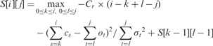where S[ − 1][ j] = 0 and S[i][-1] = −∞, ∀ i,j ≥ 0. This results in an O(m²n²) algorithm, for an optical map with m fragments and a sequence with n fragments. In practice, we can avoid this worstcase runtime by using the constraint specified in Equation (1) to prune the search space.

In order to be useful in practice, the algorithm and scoring function described here were further modified to address the following issues:

• Small sequence fragments: fragments that are less than 700 bases long are excluded as they are typically absent from the optical map.

• Handling sequence ends: typically sequences do not start or end with a restriction site. For the fragments at the end of sequences we relaxed equation Equation (1) to a version where the absolute value is not taken, i.e we only test an upper bound on the length of fragments.

• Matching to a circular map: a common case in bacterial chromosomes, this requires a change to the DP formulation to allow for matches that wrap around the ends of a linearized optical map.

2.1.3 Match significance

The DP algorithm will always find a ‘best match’ between a DNA sequence and the optical map, even if the sequence does not belong to the genome (e.g. the sequence represents a contaminant or mis-assembled contig). The algorithm described above must, therefore, be augmented with a procedure for evaluating the significance of matches produced by the DP process.

The simplest approach to solving this problem is the use of a threshold on the match score to determine a significant match. The choice of a threshold is however likely to vary with the size and number of fragments. An explicit model for random matches can lead to a more elegant solution in terms of P-values (probability that a random match has a greater score) that are comparable between sequences. A match can then be deemed significant if its P-value is less than a user-specified threshold, say x, with the useful property that the false positive rate is then guaranteed to be less than x.

A convenient model for random matches involves aligning random permutations of the in silico fragments (minus the ends) corresponding to a given sequence. Computing the significance of a match then transforms into a permutation test where we use the distribution of match scores for permutations of the sequence fragments to compute a P-value i.e. P(score of permuted sequence ≥ score of sequence). For sequences with many fragments, we estimate the distribution by sampling from the space of possible permutations, and for sequences with very few fragments (≤ 3) we skip the test entirely. This procedure has the advantage that it accurately models the distribution of fragment sizes and takes into account the structure of the scoring function. In addition, mis-assembled sequences quite often have sequence fragments in an incorrect order and the permutation test can help detect such situations.

The permutation test can be useful as a filter for poor matches and thus it also provides us with the means to choose the parameter C_σ more carefully. As mentioned in Section 2.1.1, the procedure to score matches assumes that the size of sequence fragments is largely accurate in order to suggest a value for C_σ. In the datasets we analyzed, we found many cases where the size of sequence fragments was quite different from that of the corresponding optical map fragments (an example of this can be seen in Fig. 3). Setting C_σ too conservatively may miss too many matches (as shown in Section 3) while the converse may lead to many false matches. In practice, the following coarse-grained search procedure works well to independently choose C_σ for each sequence: over the interval [4,12] set C_σ to the smallest integer that leads to a significant match.

Fig. 3.

Disagreement between sequence and optical map fragment size. Note that comments following Figure 2 also apply here. Here we show part of a real alignment for a dataset described in Section 3. The sizes of the two large sequence fragments in the middle (31.0 and 25.5 kbp) do not agree well with the optical map.

2.1.4 Non-unique matches

We expect sufficiently large sequences with many restriction sites to match uniquely to the optical map. Unique placement is, however, not possible for sequences contained in repeats, and for sequences containing few restriction sites especially if the sizes of the restriction fragments occur commonly in the optical map. In such situations, we wish to identify a set of matches that are ‘comparably good’ and remove from consideration those that are too poor to be correct. In Section 2.2, we will describe an algorithm that further refines this set of matches, to determine the placement of sequences that do not have a unique mapping.

To identify ‘comparably good’ matches, we take into account the χ² score of matches with the same number of matched restriction sites (m_r). If and are the scores for the best match and some other match, respectively (involving n_best and n_other sets of fragments), then we can use the fact that 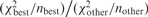has an F-distribution to filter matches that have a low score compared to the best match (based on a P-value threshold). Sequences that have multiple good matches after the filtering step are then labeled as ‘non-unique’. Note that sequences with good matches (based on m_r) that only match one restriction site are always labeled non-unique. Finally, we do not apply the uniqueness test to sequences that do not have a significant match based on the permutation test.

2.2 Sequence placement

The sequence matching procedure provides us with possible matches to the optical map but the placements that they suggest may not be mutually consistent. For example, sequences that overlap on the optical map but do not have any sequence similarity in the overlap region indicate problems with sequence placement. Under the assumption that sequences cannot overlap, the problem of choosing a good placement can be modeled as follows: let M_i be the set of matches (intervals of the optical map) corresponding to sequence i, then we wish to select a set P⊆∪_iM_i such that ∀i,|P∩M_i| = 1 and for a,b∈P,a∩b = ∅.

The Sequence Placement problem is analogous to a well-studied problem in the field of Operations Research called Interval Scheduling (Kolen et al., 2007). In a typical formulation of Interval Scheduling, we are given a set of jobs and the time intervals to which they can be assigned/scheduled, where each possible assignment has an associated weight as a measure of its goodness. We then wish to find a schedule (i.e. an assignment of jobs to time intervals that do not overlap) that is of maximal total weight. Translating ‘sequences’ to ‘jobs’ and ‘matches to the optical map’ to ‘scheduling in a time interval on a processor’, we can see that Sequence Placement is just a special case of the Interval Scheduling problem. In fact, this case is well-known to be a computationally hard problem (NP-complete) and several approximation algorithms have been proposed in the literature (Bar-Noy et al., 2001). The following simple greedy algorithm [a special case of the algorithm proposed in (Bar-Noy et al., 2001)] can be shown to be a 2-approximation:

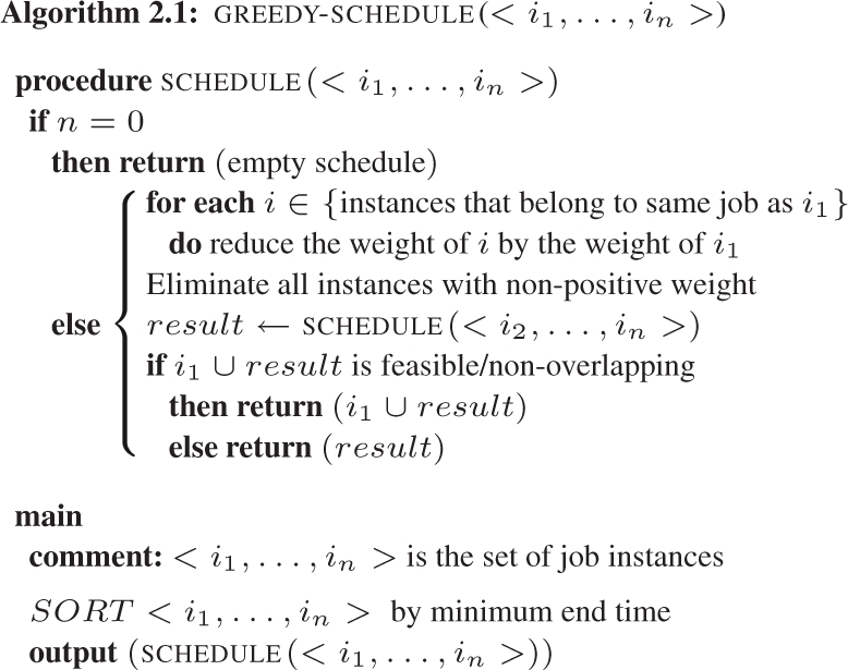
In practice we expect the greedy algorithm to return much better solutions than the provable 2-approximation bound. Also, for small problem instances, an exact algorithm based on a depth-first search to enumerate schedules/placements and find the best one, may be feasible. Based on a lower bound for the weight of the optimal schedule (that can be obtained, for example, by running the greedy algorithm), the search tree can also be conservatively pruned using the following heuristic: a subtree is pruned if weight of partial schedule + weight of instances to schedule <lower-bound. We present the results of our experiments with these two methods (GREEDY and ASTAR, respectively) in Section 3.3.

The methods presented here are general enough to handle weight functions other than the obvious one where all matches are assigned a weight of one. This can prove to be useful in two cases. In the first case, there is more than one solution that places all the sequences on the optical map and we then wish to choose a placement that preferentially places sequences in regions where they match well. This requires a scoring function for matches that is comparable across sequences, such as the P-values based on the permutation test. A two-stage weight function similar to the one in Section 2.1.1 can then help enforce the constraint that we want to maximize the number of placed sequences. In the second case, there is no solution that maps all the sequences to the optical map. Here, we might be interested in finding the solution that covers as much of the optical map as possible, i.e. the weight function is the size of the sequence. We further explore the utility of these scoring functions in Section 3.3.

In addition to GREEDY and ASTAR, we also experimented with a conservative, heuristic approach to place sequences (match filtering). This procedure iteratively places sequences which have a unique significant match, filtering out matches for other sequences that overlap the placed sequences. This process is repeated until either all sequences have been placed or all unplaced sequences have non-unique placements. Match filtering is based on the intuition that unique significant matches are likely to be correct. This is also borne out in our experiments with simulated data as shown in Section 3.

3 RESULTS

3.1 Datasets and parameters

To validate our methods we used optical maps and sequences for two bacterial strains: Yersinia aldovae ATCC 35236 and Yersinia kristensenii ATCC 33638 (that we abbreviate as YA and YK, respectively). The optical maps for these strains were generated at Opgen (www.opgen.com) using the restriction enzyme AflII. Each individual map represents the consensus of maps generated from a randomly sheared set of fragments, assembled together using the program gentig (Anantharaman et al., 1997, 1999). These strains were generated using 454 sequencing and the newbler assembler (www.454.com). Newbler generates non-overlapping contigs, and also provides information indicating the potential adjacency of pairs of contigs. More generally, many assemblers provide various forms of linking information between contigs, conceptually forming a ‘contig graph’. We use this information in a pre-processing step to identify simple paths in the graph corresponding to sets of contigs whose relative placement is unambiguous (Fig. 4a). The contigs within a simple chain are treated as a single unit throughout our algorithms. Forked paths as shown in Figure 4b indicate ambiguities due to repeats, that can be resolved using optical maps as will be discussed in Section 4. Additional information about the optical maps and the assemblies of the two Yersinia genomes is provided in Table 1. Note that Y.kristensenii and Y.aldovae have 42 and 58 sequences, respectively, with more than two restriction sites, providing an upper bound on the number of contigs we can expect to scaffold. The results shown in Tables 3 and 5 should be evaluated against these upper bounds.

Fig. 4.

Two structures identified in assembly graphs. The chain in (a) is unambiguous: the three contigs can be inferred to be adjacent. In (b) the relative order of the five contigs is ambiguous due to a repeat (contig 0406).

Table 1.

Optical Map and Sequence statistics

Strain	Map type	Coverage	No. of sites	# Contigs (N50 in kbp)	Total size (in Mbp)
YK	Optical	>40X	350	1	4.63
	454 Contigs	∼16X	404	488 (100)	4.68
YA	Optical	>40X	360	1	4.30
	454 Contigs	∼19X	411	375 (66)	4.32

Note that contigs on simple paths in the assembly graph (inferred from newbler output) were merged into 463 and 361 contigs, respectively, for YK and YA.

Table 3.

Match results for real datasets

Experiment	Program	Strain	Not significant	Not unique	Conflicts
1	Cσ = 4	YK	0	3	17
		YA	0	2	19
2	Cσ = 4	YK	19	11	0
	PT, FT	YA	19	24	0
3	PT, NU	YK	2	10	0
		YA	1	27	0
4	PT, FT	YK	2	10	0
		YA	1	27	0

The symbols PT/FT in the experiment column indicate whether or not the permutation test/F-test was performed. The symbol NU indicates that we filtered for non-unique matches. The ‘Conflicts’ column reports the number of pairs of sequences that overlap in placement but have no sequence overlap.

Table 5.

Final scaffolding statistics

Strain	# contigs	Sizes (kbp)			Total size in Mbp (% of genome)
		Min.	Mean	Max.
YK placed	39	20	108	307	4.2 (91%)
YK unplaced	424	0.08	1.2	41	0.5 (9%)
YA placed	49	2.5	71	272	3.5 (81%)
YA unplaced	312	0.01	2.6	70	0.8 (19%)

For each genome we report aggregate statistics for the contigs in the final scaffold (placed) and the contigs that could not be scaffolded (unplaced). Numbers refer to contigs obtained after collapsing simple chains in the contig graph.

To extensively test our methods, we also generated collections of artificial datasets that mimic the features of real data. These data were generated for the two Yersinia strains (X), at different levels of sizing (C) and sequencing errors (p). Each collection contained 100 datasets generated as follows: an artificial map was obtained as a random permutation of the real map corresponding to strain X. The contigs were then placed end-to-end (in a random order) on the artificial optical map to define contig locations on the map and transfer restriction site locations from the map to the sequences. Further, we introduced errors in the restriction sites by omitting individual sites with probability P and inflating sequence fragments by a factor of C. We experimented with different values of C and p to test the robustness of our methods to errors.

For sequences with six or more fragments the permutation test was performed with 200 random samples (all permutations were enumerated in the other cases). The permutation test was not applied to sequences with < 3 fragments and C_σ was set to 12 in these cases. The significance threshold for the permutation test was set to 0.005 to eliminate sequences for which even a single permuted sequence scores better. The threshold for the F-test was set to 0.01.

3.2 Robustness of the matching algorithm

The tests on simulated data allowed us to check the robustness of our methods in a setting where we know the answer. In the case of tests with C = 0, p = 0, they provide a quick sanity check. As can be seen from Experiment 1 in Table 2, and as expected, the DP matching algorithm provides perfect placements in this case. With the introduction of sizing errors, however, this is no longer the case (see Experiment 2). Finally, when restriction sites are missing, the placement accuracy can be quite low (< 80%, see Experiment 3). The value of our methods is demonstrated in Experiments 4 and 5; adding the permutation test and the test for non-uniqueness of matches reinstates the high reliability of the matches. Finally, as can be seen from Experiment 6, the reliability of our methods is robust to the addition of even large (systematic) sizing errors in the optical map. In contrast, an approach based on a fixed C_σ would be unable to handle this dataset (e.g. with C_σ = 4 we get 5% accuracy).

Table 2.

Match results for simulated datasets

Experiment	Program	Strain, C, p	Conflicts	Not significant (%)	Not unique (%)	Correctly placed (%)
1	Cσ = 4	YK, 0, 0.0	0	0	0	100
		YA, 0, 0.0	0	0	0	100
2	Cσ = 4	YK, 2, 0.0	11	0	0	89
		YA, 2, 0.0	13	0	0	85
3	Cσ = 4	YK, 2, 0.1	15	0	1	82
		YA, 2, 0.1	19	0	1	78
4	PT, FT	YK, 2, 0.0	0	1	28	100
		YA, 2, 0.0	0	1	34	100
5	PT, FT	YK, 2, 0.1	2	3	31	94
		YA, 2, 0.1	2	3	38	95
6	PT, FT	YK, 4, 0.0	0	1	27	100
		YA, 4, 0.0	0	2	34	99

The symbols PT/FT in the program column indicate whether or not the permutation test/F-test was performed. In all cases, C_σ was either set to four or we used a search procedure to set it as described in Section 2.1.3. Here we assume that sequences that have a unique, significant match are placed accordingly. On average each dataset had more than 40 sequences that were considered. The ‘Conflicts’ column reports the number of pairs of sequences that had overlapping placement but no sequence overlap. The values reported are averages over all datasets.

Our results on real data are summarized in Table 3. As can be seen from Experiment 1, without the permutation test or a filter for non-unique matches, the best matches have numerous overlaps that have no sequence support, suggesting that they are poorly placed. Introducing the permutation test and the filter for non-unique matches improves the reliability of the results (Experiment 2). However, many possible matches are omitted for not being significant. The search procedure described in Section 2.1.3 allows us to find many more significant matches (Experiment 3) and get an estimate of the degree of assembly errors in the sequences (in the form of the value of C_σ for which a significant match can be obtained). Manual inspection of the sequences with no significant match also confirmed that they indicate cases of mis-assembly.

3.3 Accuracy of sequence placement

To test our scheduling algorithms we ran them on the sequences with non-unique placement from experiments similar to those in Table 2 (See Table 4 for details). On average these test sets had 23 and 44 non-unique matches (corresponding to 10 and 15 sequences), respectively, for Y.kristensenii and Y.aldovae and we were able to run ASTAR in a reasonable amount of time in most cases. Since the computation of P-values based on permutations is expensive we used the P-values from the F-test as the weight function. We present some of the results from our experiments in Table 4. As expected, ASTAR has higher accuracy and coverage compared to GREEDY, over a wide variety of conditions (though only slightly). Despite this, GREEDY clearly does much better than its theoretical worst case (in terms of the optimization function). As is evident from Experiment 2, however, this may not be accurate enough for reliable assembly and the match filtering procedure is a valuable tool to ensure higher accuracy in sequence placement.

Table 4.

Placement results for simulated datasets

Experiment	Strain, C, p	GREEDY		ASTAR		Match filtering
		Cov.	Acc.	Cov.	Acc.	Cov.	Acc.
1	YK, 2, 0.00	0.82	0.89	0.84	0.89	0.79	0.99
	YA, 2, 0.00	0.73	0.84	0.82	0.84	0.59	0.98
2	YK, 2, 0.05	0.72	0.80	0.78	0.80	0.56	0.93
	YA, 2, 0.05	0.67	0.72	0.69	0.73	0.42	0.91
3	YK, 4, 0.00	0.73	0.81	0.80	0.81	0.67	0.96
	YA, 4, 0.00	0.70	0.75	0.74	0.75	0.62	0.96

In all cases the placement algorithms were applied to the set of unplaced sequences left after applying the matching procedure with permutation and F-test. Note that we use the following definitions: Accuracy (Acc.) = # of correct placements/# of placements by program and Coverage (Cov.) = # of correct placements/# of sequences to be placed. The values reported are averaged over all datasets.

Using real data, Experiment 3 in Table 3 resulted in 19 and 101 non-unique matches, respectively, for Y.kristensenii and Y.aldovae. With the addition of the F-test, the results remain the same but the number of matches was reduced to 18 and 89, respectively. Similar evidence for the utility of the F-test was also seen in the tests with the artificial datasets. Reducing the number of matches is important as it may allow us to run ASTAR and possibly get better placements. The final scaffolding results are shown in Table 5. We were able to run ASTAR for Y.kristensenii and thus place eight out of nine sequences that were considered. In combination with the sequences that were uniquely placed by sequence matching (39 in total), these sequences cover 4.2 Mbp of the genome (with an optical map of 4.6 Mbp or more than 91% of the genome). For Y.aldovae, we were unable to run ASTAR to completion (> 8 h) and instead we ran GREEDY to place 19 of the 25 sequences that were considered. This resulted in a sequence coverage of 3.5 Mbp (49 sequences) for a map of size 4.3 Mbp (or 81% of the genome).

4 APPLICATIONS AND FUTURE WORK

The results of the experiments in Section 3 strongly suggest that our methods are robust to sequencing and assembly errors in the sequence data. This allows us to reliably place sequences on the optical map. The combination of sequence matching and match filtering allows us to place nearly all the sequences with more than two restriction sites (that it can reasonably be expected to place uniquely). Depending on the characteristics of the genome and the optical map, this can also lead to high coverage of the optical map (as is the case for Y.kristensenii).

There are several avenues for improving genomic coverage using the tools described here. An obvious approach is to use multiple optical maps to ensure that all sequences can be reliably placed. Matching sequences to any one map is independent of the other maps (in the absence of correspondence information) and can be performed using the matching algorithm described here. Sequence placement, however, would ideally incorporate the constraints of both maps, requiring the development of new tools for this purpose.

As discussed in Section 3, the assembly graph contains valuable information about the order of sequence placements, information that we are interested in combining with the optical map data. This is a promising avenue to increase genomic coverage, especially when placing small sequences. One potential approach considers all possible paths through the assembly graph as putative sequences and evaluates their match to the optical map using the methods presented here. Paths that are not valid would, in theory, not lead to a significant match and can therefore be excluded. However, for complicated assembly graphs, this procedure can be computationally prohibitive and we are currently working on more direct ways to achieve this goal. Another approach to be considered is to use unique matches to the optical map as ‘anchors’ that determine distance constraints within the assembly graph. Paths that satisfy these constraints then give us possible reconstructions of the genome.

Finally, the methods presented here were constrained by the fact that the restriction enzymes chosen to construct the optical maps might not be optimal in terms of informing the sequence placement process. An ideal choice of restriction enzyme would provide distinct restriction site patterns on the sequences and lead to confident placement even in the presence of errors. This is clearly a genome-specific choice and should be done after assembly. The choice of an enzyme is further constrained by bio-chemical and computational considerations involved in constructing the optical map. Designing an algorithm for choosing a restriction enzyme that satisfies such constraints is an interesting avenue for future research.

REFERENCES

- Anantharaman TS, et al. Genomics via optical mapping. ii: ordered restriction maps. J. Comput. Biol. 1997;4:91–118. doi: 10.1089/cmb.1997.4.91. [DOI] [PubMed] [Google Scholar]
- Anantharaman T, et al. Genomics via optical mapping. iii: contiging genomic DNA. In: Lengauer T, et al., editors. Proceedings of the Seventh International Conference on Intelligent Systems for Molecular Biology. Vol. 7. AAAI Press; 1999. pp. 18–27. [PubMed] [Google Scholar]
- Antoniotti M, et al. Genomics via Optical Mapping iv: Sequence Validation via Optical Map Matching. Technical Report. 2001 CIMS TR-811, Courant Institute of Mathematical Sciences, NYU, March 2001. [Google Scholar]
- Bar-Noy A, et al. A unified approach to approximating resource allocation and scheduling. J. ACM. 2001;48:1069–1090. [Google Scholar]
- Ben-Dor A, et al. The restriction scaffold problem. J. Comput. Biol. 2003;10:385–398. doi: 10.1089/10665270360688084. [DOI] [PubMed] [Google Scholar]
- Engler FW, et al. Locating sequence on fpc maps and selecting a minimal tiling path. Genome Res. 2003;13:2152–2163. doi: 10.1101/gr.1068603. [DOI] [PMC free article] [PubMed] [Google Scholar]
- Goldberg S.MD, et al. A sanger/pyrosequencing hybrid approach for the generation of high-quality draft assemblies of marine microbial genomes. Proc. Natl Acad. Sci. 2006;103:11240–11245. doi: 10.1073/pnas.0604351103. [DOI] [PMC free article] [PubMed] [Google Scholar]
- Kolen A.WJ, et al. Interval scheduling: a survey. Nav. Res. Logist. 2007;54:530–543. [Google Scholar]
- Latreille P, et al. Optical mapping as a routine tool for bacterial genome sequence finishing. BMC Genomics. 2007;8:321–326. doi: 10.1186/1471-2164-8-321. [DOI] [PMC free article] [PubMed] [Google Scholar]
- Margulies M, et al. Genome sequencing in microfabricated high-density picolitre reactors. Nature. 2005;437:376–380. doi: 10.1038/nature03959. [DOI] [PMC free article] [PubMed] [Google Scholar]
- Nathans D, Smith HO. Restriction endonucleases in the analysis and restructuring of DNA molecules. Annu. Rev. Biochem. 1975;44:273–293. doi: 10.1146/annurev.bi.44.070175.001421. [DOI] [PubMed] [Google Scholar]
- Pop M. Shotgun sequence assembly. Adv. Comp. Vol. 60. 2004;60:193–248. [Google Scholar]
- Pop M, et al. Hierarchical scaffolding with bambus. Genome Res. 2004;14:149–159. doi: 10.1101/gr.1536204. [DOI] [PMC free article] [PubMed] [Google Scholar]
- Reslewic S, et al. Whole-genome shotgun optical mapping of rhodospirillum rubrum. Appl. Environ. Microbiol. 2005;71:5511–5522. doi: 10.1128/AEM.71.9.5511-5522.2005. [DOI] [PMC free article] [PubMed] [Google Scholar]
- Samad A, et al. Optical mapping: a novel, single-molecule approach to genomic analysis. Genome Res. 1995;5:1–4. doi: 10.1101/gr.5.1.1. [DOI] [PubMed] [Google Scholar]
- Soderlund C, et al. Fpc: a system for building contigs from restriction fingerprinted clones. Bioinformatics. 1997;13:523–535. doi: 10.1093/bioinformatics/13.5.523. [DOI] [PubMed] [Google Scholar]
- Valouev A, et al. Alignment of optical maps. J. Comp. Biol. 2006;13:442–462. doi: 10.1089/cmb.2006.13.442. [DOI] [PubMed] [Google Scholar]
- Zhou S, et al. A whole-genome shotgun optical map of yersinia pestis strain kim. Appl. Environ. Microbiol. 2002;68:6321–6331. doi: 10.1128/AEM.68.12.6321-6331.2002. [DOI] [PMC free article] [PubMed] [Google Scholar]
- Zhou S, et al. Shotgun optical mapping of the entire leishmania major friedlin genome. Mol. Biochem. Parasitol. 2004;138:97–106. doi: 10.1016/j.molbiopara.2004.08.002. [DOI] [PubMed] [Google Scholar]