Identification of related proteins with weak sequence identity using secondary structure information

Abstract

Molecular modeling of proteins is confronted with the problem of finding homologous proteins, especially when few identities remain after the process of molecular evolution. Using even the most recent methods based on sequence identity detection, structural relationships are still difficult to establish with high reliability. As protein structures are more conserved than sequences, we investigated the possibility of using protein secondary structure comparison (observed or predicted structures) to discriminate between related and unrelated proteins sequences in the range of 10%–30% sequence identity. Pairwise comparison of secondary structures have been measured using the structural overlap (Sov) parameter. In this article, we show that if the secondary structures likeness is >50%, most of the pairs are structurally related. Taking into account the secondary structures of proteins that have been detected by BLAST, FASTA, or SSEARCH in the noisy region (with high E value), we show that distantly related protein sequences (even with <20% identity) can be still identified. This strategy can be used to identify three-dimensional templates in homology modeling by finding unexpected related proteins and to select proteins for experimental investigation in a structural genomic approach, as well as for genome annotation.

To exploit the data resulting from knowledge of complete genomes, the need for simple and reliable tools to predict structural features (two- [2D] or three-dimensional [3D]) of new proteins is paramount. Biologists and biochemists often require structural models at their disposal to interpret experimental data. Currently, three different methods are being developed to predict the 3D structures of proteins: first, standard comparative homology modeling in which the structures of homologous proteins are used as starting points; second, the threading approach in which sequences are checked for their fold compatibility using empirical target functions that are not yet fully optimized; and third, de novo structure prediction in which structures are directly derived using empirical rules and simplified protein models. With the development of structural genomics, homology molecular modeling will yield an increasing number of potential protein templates. However, molecular modeling of proteins is confronted with the problem of finding homologous proteins, especially if their sequences share <30% identity. The main problem is to identify whether two proteins are homologous even if no significant similarities can be detected by pairwise sequence comparison. Some strategies have been proposed to address this problem (for review, see Teichmann et al. 1999). In the first approach, as the homology is transitive, an intermediate protein sequence can be used as a similarity relay (Park et al. 1997, 1998; Teichmann et al. 2000). In this context, multiple alignments performed with divergent protein sequences (Taylor 1986) may also provide some information. The second approach is the improvement in searching algorithms, as has been done with PSI-BLAST (Altschul et al. 1997) or with profile methods (Gribskov et al. 1987). More recently, secondary structure information has also been used for protein fold recognition (Hargbo and Elofsson 1999; Jones et al. 1999; Kelley et al. 2000).

In this article, we revisit the possibility of using secondary structure likeness to address this problem. We show that secondary structure agreement between predicted secondary structures of template and query proteins can be used to identify distantly related protein sequences. This efficient template detection allows the modeling process to be applied with improved reliability even in the twilight zone of 10%–30% sequence identity.

Results

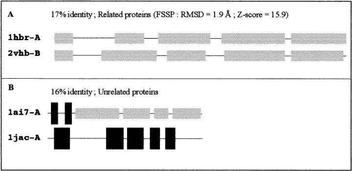
The main idea was to check if the comparison of secondary structures (either observed or predicted) could provide valuable information for the detection of 3D-related proteins with poor sequence similarity. A typical example for two structurally related proteins (1hbr-A and 2vhb-B) and two unrelated proteins (1ai7 and 1jac) is illustrated in Figure 1 ▶. Both sequence pairs share ∼16% identity, and these proteins could not be assigned as homologous pairs on the basis of sequence identity. However, they could easily be classified by comparing their observed secondary structures. To look at the possibility of generalizing this observation, an extensive comparison of the secondary structures of a large number of sequence pairs was performed.

Fig. 1.

Comparison of two related (A) and unrelated (B) protein pairs at the secondary structure level. The sequence pairs of 1hbr-A/2vhb-B (A) and 1ai7/1jac (B) were aligned using the CLUSTALW (1.8) program (Thompson et al. 1994) with default parameters and their observed secondary structures were deduced from PDB files using the DSSP algorithm (Kabsch and Sander 1983). Helices are in thin light boxes, and sheets are in large dark boxes.

Sequence pair sets

For a given searching algorithm, FASTA, SSEARCH, or BLAST, the first step was to collect all pairs of sequences with known structures in the 10%–50% sequence identity range and to look at their secondary structure likeness. This was done using each protein of the pdb_select_25 (Hobohm and Sander 1994) as a query sequence in an all-to-all comparison search against the pdb_select_95 and by comparing their observed secondary structures. This method was also applied to higher E values than the default ones to identify homologous proteins sharing few identities. The FSSP database (Holm and Sander 1994) was used to identify true positive pairs. The results are given in Table 1 for the three different similarity search methods with E values of 10, 100, or even 1000 for BLASTP. The total number of hits (i.e., sequence pairs with <50% identity) comprised between 1211 and 4453 hits. The average identity between sequence pairs ranged from 21.4 to 30.1, and the average length of pairs was rather constant (from 141 to 168 amino acids). As expected, the lower the E value, the lower the number of hits and the higher the percentage of true positives. For an E value set to 10, the percentage of true positives (3D similar) ranged from 64.7% (SSEARCH) to 96.1% (BLAST), whereas the percentage of false positive ranged from 35.3% and 3.9%. Logically, for a higher E value (100 for FASTA and SSEARCH, 1000 for BLAST), the order was inverted because more noise was introduced in the search process. Table 2 shows the distribution of pairs in the 10%–30% identity range. Obviously, the average identity level was lower than that for the 10%–50% identity range, and it ranged between 19.8% and 23.9%. The average length was slightly lower (from 135 to 163 amino acids, depending on both algorithm and E value). In the 10%–30% identity range, the percentage of structurally similar proteins decreased, whereas the percentage of dissimilar ones increased.

Table 1.

Distribution comparison of sequence pairs between 10% and 50% identity detected with different E values

	BLAST (E = 10)	BLAST (E = 1000)	FASTA (E = 10)	FASTA (E = 100)	SSEARCH (E = 10)	SSEARCH (E = 100)
Number of selected pairsa	1243	1841	1211	2992	1471	4453
Structurally similar (%)b	96.1	74.7	70.5	44.4	64.7	26.5
Structurally dissimilar (%)	3.9	25.3	29.5	65.6	35.3	73.5
Average alignment length	176	158	168	143	164	141
Average identity rate (%)	30.1	27.1	27.4	22.6	25.9	21.4

E is the expected E value as defined in Altschul et al. (1997).

^a All pairs sharing between 10% and 50% identity, >50 residues and exhibiting <10% gaps.

^b Structurally similar pairs are proteins present in the FSSP database with a Z score > 2 and with at least 100 amino acids.

Table 2.

Distribution comparison of sequence pairs between 10% and 30% identity detected with different E values

	BLAST (E = 10)	BLAST (E = 1000	FASTA (E = 10)	FASTA (E = 100)	SSEARCH (E = 10)	SSEARCH (E = 100)
Number of selected pairsa	765	1316	852	2634	1115	4097
Structurally similar (%)b	93.6	66	58.1	25.1	53.5	20.1
Structurally dissimilar (%)	6.4	34	41.9	74.9	46.5	79.9
Average alignment length	163	145	151	135	149	135
Average identity rate (%)	23.9	22.4	22.1	20.3	21.5	19.8

E value is the expected value as defined in Altschul et al. (1997).

^a All pairs sharing between 10% and 50% identity, >50 residues and exhibiting <10% gaps.

^b Structurally similar pairs are proteins present in the FSSP database with a Z score > 2 and with at least 100 amino acids.

Observed versus observed secondary structure compatibility

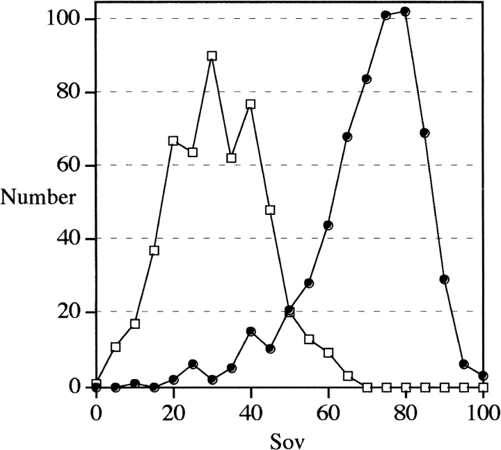
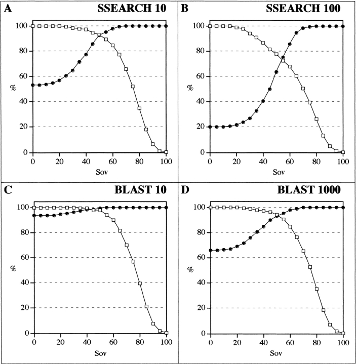
To define the function to be used to accurately estimate comparability between secondary structures, we first used secondary structures calculated from 3D structures using the DSSP method. In Figure 2 ▶, the agreement between observed secondary structures (as measured by the Sov parameter) is plotted as a function of identity (Fig. 2A ▶) or similarity (Fig. 2B ▶) for both related and unrelated protein sequences. As expected, all pairs sharing >30% identity were structurally similar and, logically, for these pairs the Sov parameter was generally >60%. In contrast, in the 10%–30% identity range, the number of true pairs represented only about half the whole set (53%). However, in this identity range, a clear separation between true and false positive pairs was obtained using the Sov parameter. If sequence similarities were considered instead of identities, the scores increased by ∼20%, thus giving rise to a 30%–50% similarity range. However, the same observation could be made about true versus false distributions. Therefore, only selected sequence pairs, exhibiting between 10% and 30% identity for which ambiguities remained in the structural assignment, were considered in subsequent sections of this article. The numbers of true and false pairs are plotted in Figure 3 ▶ as a function of the Sov value obtained with the SSEARCH algorithm. Their distributions are centered on Sov values of 30% and 77% for false pairs and true pairs, respectively. For example, when a minimum likeness between observed secondary structures was fixed at 50%, the number of true pairs was as high as 555 when compared with a total number of 600 pairs, giving rise to a recognition rate of 93%. This type of distribution could be used to plot the percentage of coverage and detection as a function of Sov parameters (Fig. 4 ▶). The relationships between the coverage rate and the detection rate of true positives as a function of Sov were investigated with the SSEARCH and BLAST programs using different E values (Fig. 4 ▶). In all cases, the detection rate increased in accord with the Sov value calculated from observed secondary structures. Three different regions of Sov could be distinguished: the first region with Sov < 30%, in which pairs were unrelated in most cases; a second region with Sov > 70%, in which pairs were related in most cases; and a third, transition region in the range 30% < Sov < 70%. The Sov value region that showed the largest variation in detection and coverage was between 30% and 70% regardless of the method of comparison and the associated E value. Typically, such calibration curves provide the biologist with a confidence index when the user is searching for a 3D template for molecular modeling.

Fig. 2.

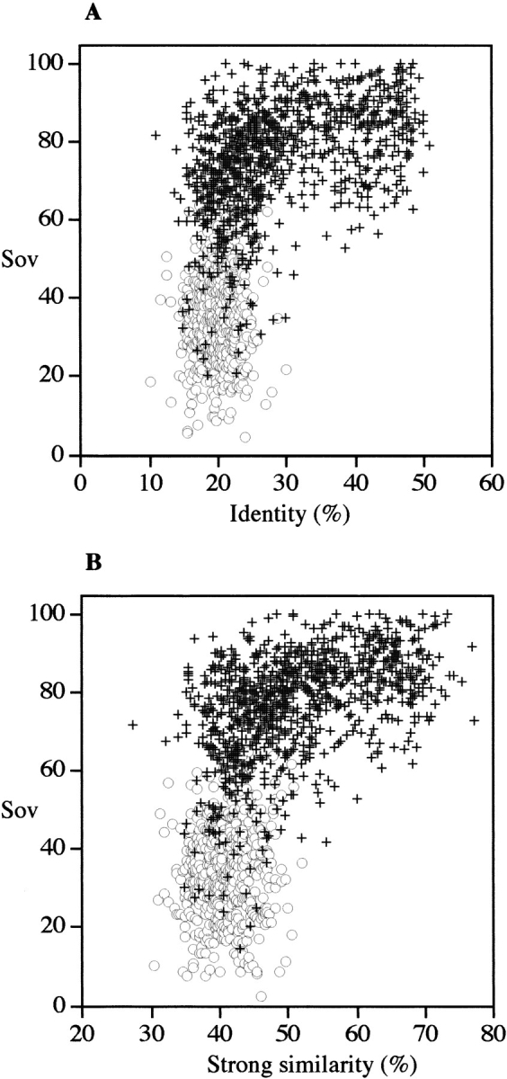
Distribution of aligned sequence pairs as a function of the agreement between observed secondary structures. Each sequence pair (query and subject detected in pdb_select_95 with the SSEARCH algorithm with an E value = 10) has been aligned using CLUSTALW (1.8) with default parameters (see Materials and Methods). The observed secondary structures were deduced from corresponding PDB files using the DSSP program (Kabsch and Sander 1983). Agreement in secondary structure was measured using the Sov parameter (Zemla et al. 1999). False positive pairs, open pale circles; true positive pairs, black crosses. Identity (A) and strong similarity as defined in CLUSTALW (B).

Fig. 3.

Number of false positive pairs (empty squares) and true positive pairs (filled circles) as a function of observed secondary structure overlap (Sov). Each sequence pair (query and subject detected in pdb_select_95 with the SSEARCH algorithm with an E value = 10) has been aligned using CLUSTALW (1.8) with default parameters (see Materials and Methods). The observed secondary structures were deduced from corresponding PDB files using the DSSP program (Kabsch and Sander 1983). Agreement in secondary structure was measured using the Sov parameter (Zemla et al. 1999). Only sequence pairs in the 10%–30% identity range have been taken into account.

Fig. 4.

Percentages of coverage and detection as a function of observed secondary structure overlap (Sov). The percentage of coverage (true positive pairs above a given Sov divided by the total number of true positive pairs) is shown by open squares. The percentage of detection (true positive pairs divided by total number of pairs above a given Sov) is shown by filled circles. The different algorithms used are SSEARCH with E values of 10 (A) and 100 (B) and BLAST with E values of 10 (C) and 1000 (D). Only sequence pairs (query and subject) in the 10%–30% identity range have been taken into account.

Observed versus predicted secondary structure compatibility

As the secondary structure is not known for a novel protein, the predicted secondary structure should be used instead. The agreement between several methods estimated by the Q3 parameter is presented in Table 3 for PHD (Rost and Sander 1993), DSC (King and Sternberg 1996), and SOPMA (Geourjon and Deléage 1995). In particular, when a consensus prediction of these three methods is used, the accuracy (Q3%) reaches 72.8% for the 1106 pdb_select_25 proteins. In addition, the Sov parameter increases when different methods are combined. In Figure 5 ▶, the agreement between observed (SSEARCH subject sequence) and predicted (SSEARCH query sequence) secondary structures (as measured by the Sov parameter) are plotted as a function of sequence identity (Fig. 5A ▶) or similarity (Fig. 5B ▶) for both related and unrelated protein sequences. The distribution looks similar to that presented for observed versus observed secondary structures (Fig. 2 ▶), indicating that predicted secondary structures might also be used to choose templates for molecular modeling. However, in the case of observed versus predicted secondary structures, the dispersion was wider than that for observed versus observed secondary structures, probably because of the fact that agreement between prediction and observation was only ∼72%. To know whether predictions could be used instead of observed versus predicted secondary structures, the resemblance between predicted secondary structures for all pairs of proteins was investigated.

Table 3.

Accuracy and agreement levels of secondary structure predictions

	Q3%
Prediction method	Coil	Helix	Sheet	Average	Sov
SOPMA	75.5	75.3	62.1	72.5	66.7
DSC	78.0	64.5	56.2	68.5	61.5
PHD	74.9	74.3	64.8	72.5	67.8
SOPMA-DSC-PHDa	80.1	72.9	59.4	72.8	67.9

^a Consensus prediction from all three methods as calculated in NPS@ (Combet et al. 2000).

Fig. 5.

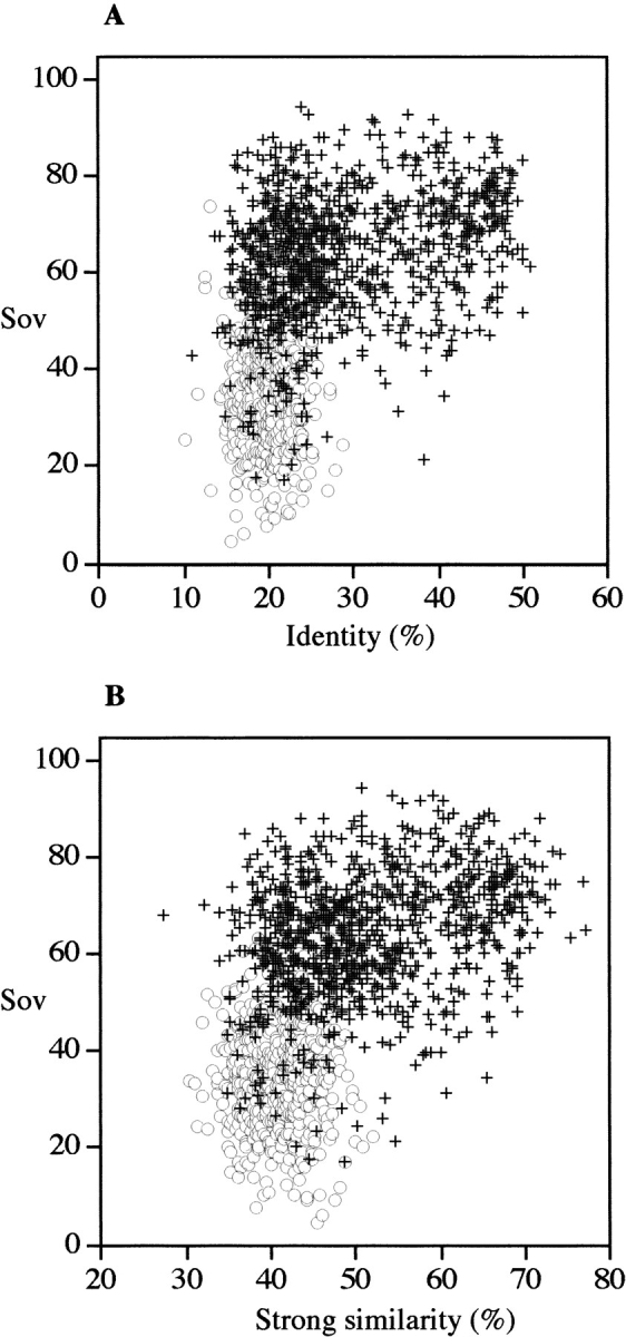
Distribution of aligned sequence pairs as a function of the agreement between observed and predicted secondary structures. Each sequence pair (query and subject detected in pdb_select_95 with SSEARCH algorithm with an E = 10) has been aligned using CLUSTALW (1.8) program with defaults parameters (see Materials and Methods). The observed secondary structures of the subject protein were deduced from corresponding PDB files by using the DSSP program (Kabsch and Sander 1983). The predicted secondary structure of the query protein was predicted by a consensus of PHD, SOPMA, and DSC (see Materials and Methods). Agreement in secondary structure was measured by using the Sov parameter (Zemla et al. 1999). False positive pairs, open pale circles; true positive pairs, dark crosses. Identity (A) and strong similarity as defined in CLUSTALW (B).

Predicted versus predicted secondary structure compatibility

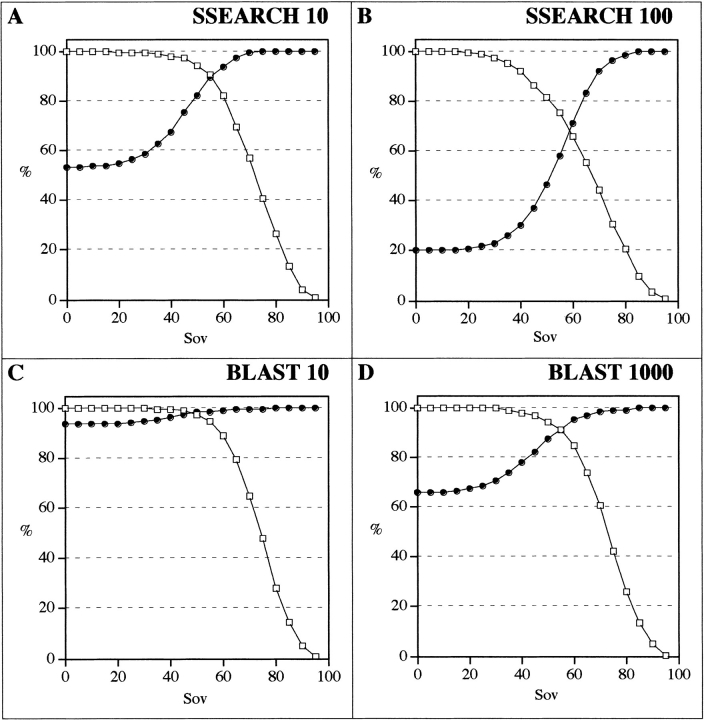
Figure 6 ▶ shows the agreement, as measured by the Sov parameter, between predicted secondary structures (SSEARCH query and subject sequences) as a function of identity (Fig. 6A ▶) or similarity (Fig. 6B ▶) for both related and unrelated protein sequences. The distribution looks closer to that presented for observed versus observed secondary structures (Fig. 2 ▶) than for observed versus predicted structures (Fig. 5 ▶), indicating that predicted secondary structures could indeed be used to increase the possibility of identifying possible templates for molecular modeling. The explanation for this good agreement is probably that even if predictions are far from perfect, they predict similar conformations for related proteins. In other words, even if the predictions are wrong, they probably fail in the same way for all related proteins. The calibration curve of coverage and success as a function of the Sov parameter is given in Figure 7 ▶ for SSEARCH (Fig. 7A,B ▶) and BLAST (Fig. 7C,D ▶). For both similarity search programs, the secondary structure brought some additional information about structural relationships, especially if high expected E values were used. For example, with a BLAST performed on pdb_select_95 with an E value of 1000, a Sov value between predicted secondary structures ≥60 yielded a coverage of 85% and a success of 95% in the detection of related pairs. This means that secondary structure resemblance is a way of detecting related pairs even in the noisy region of a BLAST search.

Fig. 6.

Distribution of aligned sequence pairs as a function of the agreement between predicted secondary structures. Each sequence pair (query and subject detected in pdb_select_95 with SSEARCH algorithm with an E = 10) has been aligned using CLUSTALW (1.8) program with defaults parameters (see Materials and Methods). The predicted secondary structure of the query and the subject protein was predicted by a consensus of PHD, SOPMA, and DSC (see Materials and Methods). Agreement in secondary structure was measured by using the Sov parameter (Zemla et al. 1999). False positive pairs, open pale circles; true positive pairs, dark crosses. Identity (A) and strong similarity as defined in CLUSTALW (B).

Fig. 7.

Percentages of coverage and detection as a function of predicted secondary structure overlap (Sov). The percentage of coverage (true positive pairs above a given Sov divided by the total number of true positive pairs) is given in open squares. The percentage of detection (true positive pairs divided by total number of pairs above a given Sov) is given in filled circles. The different algorithms used are SSEARCH with E values of 10 (A) and 100 (B) and BLAST with E values of 10 (C) and 1000 (D). Only sequence pairs in the 10%–30% identity range have been taken into account.

Application to molecular modeling

In a molecular modeling process, the secondary structure of one protein (the potential template) is known, whereas the structure of the unknown protein (the query) can at best be approximated using prediction methods. However, prediction can also be performed on the template protein, and a question that should be addressed is: Is the comparison of predicted versus predicted structures more appropriate than observed versus predicted ones in identifying homologous proteins? The number of pairs detected is shown in Table 4 for both SSEARCH and BLAST algorithms as a function of identity ranges. With SSEARCH, when no secondary structure predictions were taken into account, the percentage of correctly detected pairs was 53% and 20% for E values of 10 and 100, respectively. When a Sov value threshold of 70% was used, the number of related pairs was highest for observed versus observed structures. However, more surprisingly, the number of related pairs was much higher for predicted versus predicted pairs (341 for E = 10 and 366 for E = 100) than for observed versus predicted ones (140 for E = 10 and 153 for E = 100), regardless of the identity range. Moreover, the success rate was slightly better for predicted versus predicted (99% for E = 10) than for observed versus predicted (97% for E = 10) secondary structures. The numbers of related pairs using predicted versus predicted agreement were of the same order of magnitude as those detected using observed versus observed agreement (394 for E = 10 and 417 for E = 100). With BLAST, if no secondary structure predictions were taken into account, the percentage of correctly detected pairs was 94% and 66% for E values of 10 and 1000, respectively. By adding secondary structure information, the recognition rate increased up to nearly 100%. Moreover, the combination of high E values (E = 100 for SSEARCH and E = 1000 for BLAST) with the predicted secondary structure compatibility (measured with SOV) permits us to identify new related proteins. Indeed, for SSEARCH (E = 100), 25 new proteins have been detected (366 as compared with 341) by considering the Sov parameter. These 25 new proteins were not present in the SSEARCH (E = 10) list of hits. In the case of BLAST, up to 62 new related proteins have been detected (524 as compared with 462) that were not present in the BLAST (E = 10) list of hits. These data clearly show that even for modeling purposes, the comparison of predicted versus predicted secondary structures is more suitable than the observed versus predicted comparison.

Table 4.

Effect of secondary structure information on the detection of related pairs

	SSEARCH		BLAST
	E = 10	E = 100	E = 10	E = 1000
Without secondary structure information:a
10%–15% identity	7	21	0	0
15%–20% identity	131	238	86	143
20%–25% identity	269	366	355	411
25%–30% identity	189	197	295	314
Total	596 (53)	822 (20)	716 (94)	868 (66)
Observed versus observed secondary structures:a
10%–15% identity	2	4	0	0
15%–20% identity	70	86	43	63
20%–25% identity	168	173	228	263
25%–30% identity	154	154	231	242
Total	394 (100)	417 (98)	502 (100)	568 (100)
Observed versus predicted secondary structures:a
10%–15% identity	0	0	0	0
15%–20% identity	24	32	29	40
20%–25% identity	75	80	88	109
25%–30% identity	41	41	73	73
Total	140 (97)	153 (90)	190 (99)	222 (98)
Predicted versus predicted secondary structures:a
10%–15% identity	1	3	0	0
15%–20% identity	49	66	25	46
20%–25% identity	154	164	204	231
25%–30% identity	137	133	233	247
Total	341 (99)	366 (92)	462 (99)	524 (98)

The number in parentheses is the percentage of hits detected that are structurally related.

^a Sov threshold = 70%.

A typical example is provided in Figure 8A ▶ for two proteins (6fab-H and 1ah1) of low sequence identity (18%) and high predicted versus predicted Sov parameters (89.8%). The template was detected using PSI-BLAST on the nr databank (571,000 entries; E value of 3.1 in converged final run). The alignment of the matching regions of both sequences, performed with CLUSTALW (1.8), superposed the two structures with a RMSD of 2.3 Å. This result indicated that both folds are comparable. A 3D model of 1ah1 was built with the Modeller program using the 6fab-H structure as the template (Fig. 8B ▶). Hence, secondary structure compatibility has led to the selection of a valuable template for molecular modeling.

Fig. 8.

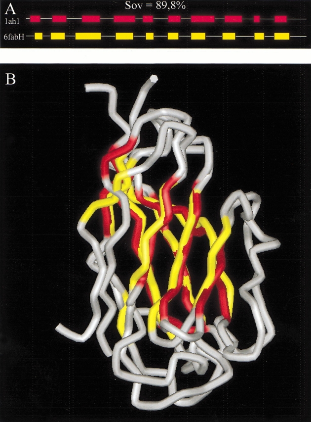
Molecular modeling of 1ah1 from 6fab-H. The sequence of the 1ah1 PDB file was used for a PSI-BLAST search (E value set to 100) onto the nr databank. After PSI-BLAST had converged (fifth run), the matching regions between the query and the first detected PDB entry (6fab-H) were aligned by CLUSTALW (1.8) with default parameters. The predicted consensus secondary structure of both sequences was obtained from the NPS@ server (A). The Sov value between predicted secondary structures is 89.8%. Superposition (B) of the 1ah1 model generated with 6fab-H as the template and the experimental 1ah1structure. Sheets are colored in red for 1ah1 and yellow for 6fab-H.

Discussion

In this article, we have shown that secondary structure prediction can help in the identification of related proteins with divergent sequences. As the structures of related proteins are often more conserved than their sequences, this conservation also exists at the level of secondary structure. In very recent studies, this conservation has been used on a residue per residue basis with a simple scoring function for the generation of secondary structure profiles (Kelley et al. 2000). However, when comparing secondary structures, comparison of secondary elements has been found to be more useful in locating secondary structure elements (Rost and Sander 1993). For this purpose, the parameter that we used is the structural overlap (Sov) parameter as originally defined by Rost and Sander (1993) and recently updated by Zemla et al. (1999). This parameter has proved to be a good indicator of the extent to which secondary structure predictions fit with the observed structure for a given protein. In this article, we have shown that this parameter is also useful in the comparison of secondary structures of two different proteins. Here, conservation in secondary structure can also be detected by the Sov function and the Sov value can be used to detect proteins with rather dissimilar sequences. Secondary structure information is particularly useful below 30% identity, as pairwise sequence comparisons detect only about half of the related proteins sharing 20%–30% identity (Park et al. 1997; Teichmann et al. 1999). Below 20% identity, this proportion is even smaller.

Secondary structure information has already been used to validate a fold recognition approach from secondary structure alignments (Russell et al. 1996; Koretke et al. 1999) or to improve the sequence-structure alignment in threading methods (Miyazawa and Jernigan 2000; Jones et al. 1999). However, these attempts used the comparison between observed (template) and predicted (target) states. In our work, we show that predicted states for both the template and the target are more appropriate than observed versus predicted states. The explanation is that for distantly related proteins, predicted states can be much closer to each other (even if predictions are 72% correct in average) than predicted and observed states.

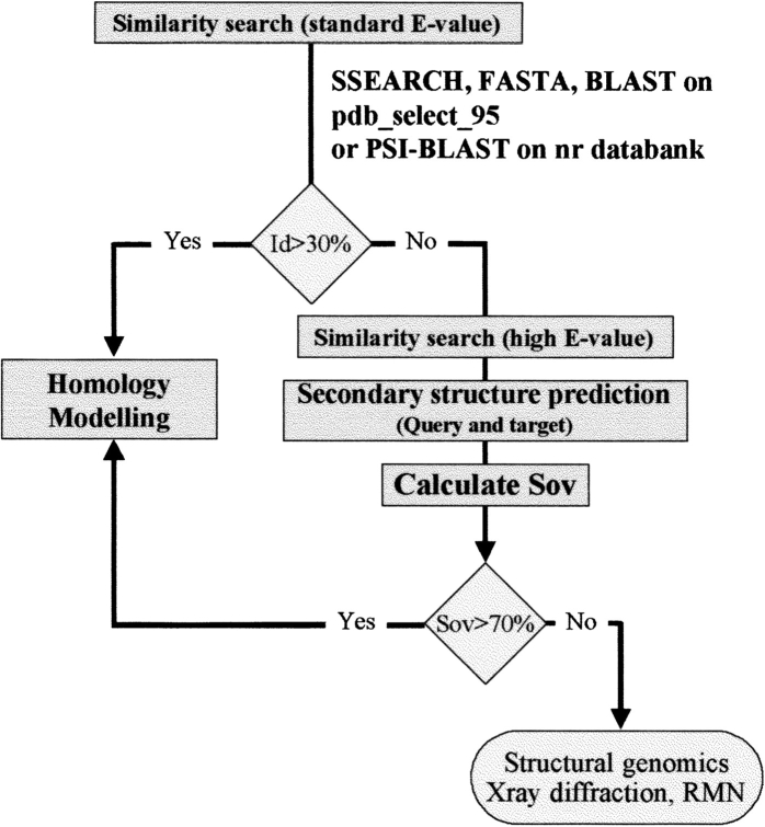
We have established that in the 10%–30% identity sequence range, when the Sov parameter is >50%, almost all proteins can be correctly assigned as structurally similar on the basis of predicted secondary structure. The secondary structure brings an additional dimension to the identity level, as for a identity level of 20%, as seen in Figure 2 ▶, Sov varies from 20% to >95%. We have also calculated calibration curves for the use of secondary structure prediction. When these are used, our approach permits an increase in the number of potential templates for molecular modeling. As an example, we have successfully built a model for a protein that has a sequence identity as low as 16% compared with its homologue. This strategy is particularly useful in molecular modeling as finding distantly related proteins may permit the modeling of more and more proteins. Another potential application could be the identification of protein families on a genomic scale. Indeed, this parameter can be used in the assignment of an unknown protein to a given family. We have also shown that this information on secondary structure is particularly useful in detecting structurally related protein sequences using similarity search algorithms with a high E value as the expected threshold. The noise that appears when SSEARCH, FASTA, or BLAST are used with high E values is largely reduced using secondary structure predictions. For example, in this study, even with a high E value (E = 1000 was used with BLAST), no additional noise appears in the detection of related protein sequences following the inclusion of secondary structure resemblance information. Even with the iterated version of BLAST (PSI-BLAST), which performs much better than BLAST in detecting remote homologies (Müller et al. 1999), the secondary structure brings additional and independent information that can be useful in the validation of the alignment (Fig. 8 ▶). This approach is particularly useful in structural genomics. The guidelines for automatic assignment of related or unrelated proteins for which the structure should be either modeled or experimentally determined are given in Figure 9 ▶. If similarity search methods with standard E values fails to detect homologous proteins (identity < 30%), a new run should be performed with higher E values (E > 100). In this latter case, the results can be filtered by the compatibility of predicted secondary structures (SOV > 70%). This strategy may allow a biologist to enter into a 3D modeling process. If no homologous proteins can be detected on the basis of sequence identity (identity < 30%) or if the agreement between predicted secondary structures (Sov < 70%), the query protein can be assigned as a structural orphan. This makes this protein attractive as a starting candidate for experimental structure determination in a structural genomics approach. Work is in progress to include the resemblance of predicted versus predicted secondary structures into fully automatic modeling procedures. A web server will be designed to automatically calculate the secondary structure agreement in BLAST and SSEARCH outputs available with the NPS@ server (http://pbil.ibcp.fr/NPSA).

Fig. 9.

General guidelines for the use of secondary structure prediction in structural genomics.

Finally, there are at least three applications for which this work can be useful. The first is to optimize or validate a pairwise alignment on the basis of secondary structures. The second is to validate the finding of a template for further molecular modeling. The last is to permit the identification of related proteins (genome annotation) from genome projects.

Materials and methods

Sequence pair building

All protein sequences in the pdb_select_25 nonredundant databank of 3D structures (Hobohm and Sander 1994) were used as the starting point. This databank contained 1106 protein chains whose structures are known and share <25% pairwise identity. Each of these chains was compared with the 3292 sequences of the pdp_select_95 databank (Hobohm and Sander, 1994) using BLASTP (Altschul et al. 1997), FASTA (Pearson and Lipman 1988), or SSEARCH (Smith and Waterman 1981). In order to explore the twilight zone of similarity, several E values were chosen before searching (E = 10 and E = 100 for FASTA and SSEARCH, E = 10 and E = 1000 for BLASTP). From the result file, aligned sequence pairs were extracted from the matching regions given by the searching algorithm.

Only aligned sequence pairs containing at least 100 amino acids, with <10% gaps and showing an identity level in the range 10%–50% were used in this study. All these sequence pairs were realigned with CLUSTALW (default parameters). In the realignment process, the observed secondary structure of the query sequence was used as a profile to weight gap penalties.

Protein structural similarity

To distinguish 3D related proteins (true positive pairs) from unrelated ones (false positive pairs), the FSSP database (Holm and Sander 1994) was used as follows: True positive pairs (i.e., structurally similar) were proteins occurring in FSSP with a Z score >2 and with at least 100 aligned amino acids. All protein sequence pairs absent in FSSP were considered as false (i.e., structurally dissimilar). Protein sequences satisfying neither of the previous conditions were discarded and no longer considered in this study.

Secondary structure

Observed secondary structures in proteins of known structure were deduced using the DSSP program (Kabsch and Sander 1983).

Secondary structures of protein sequences were predicted with the help of methods such as SOPMA (Geourjon and Deléage 1995), DSC (King and Sternberg 1996), or PHD (Rost and Sander 1993), all of which use information derived from multiple sequence alignment. Briefly, for each protein examined, the sequence was compared with BLAST to an up-to-date SWISSPROT database. First, all sequences having an E value >1.0 were discarded. Second, the bits scores were averaged onto the remaining sequences. All sequences having a bit score above the mean value were retained. Third, within this set of sequences, a minimal ratio of 10 between the E values of two sequences was necessary to submit proteins to multiple alignment. This ensured a relatively good representation of the bits score range. Thereafter, this set of sequences plus the query sequence was submitted to CLUSTALW (Thompson et al. 1994). The resulting alignment was used in the secondary structure prediction methods as originally described by the authors. A consensus of the SOPMA, DSC, and PHD methods available from the NPS@ Web server (http://pbil.ibcp.fr/NPSA; Combet et al. 2000) was used. Only three states were taken into account (helix, sheet, and coil) to validate the consensus, as all methods used in this study were capable of predicting at least these three states. The accuracy of secondary structure prediction methods was estimated using either the percentage correct (Q3) or the structural overlap (Sov) parameter.

Secondary structure agreement

For each aligned sequence pair, the agreement between secondary structures was estimated by calculating the Sov parameters (Rost et al. 1994) as most recently defined (Zemla et al. 1999); that is,

1

in which len is the segment length; H, E, C are helix, extended, and coil states; minov is the length of actual secondary structures overlap of the query s_q and the target s_t; maxov is the maximal length of overlapping secondary structures s_q and s_t; and δ is defined as

2

Molecular modeling

Molecular modeling was performed using spatial restraints with the help of the default procedure (model-default) of the Modeller program (Sali and Blundell 1993).

References

- Altschul, S.F., Madden, T.L., Schaffer, A.A., Zhang, J., Zhang, Z., Miller, W., and Lipman, D.J. 1997. Gapped BLAST and PSI-BLAST: A new generation of protein database search programs. Nucleic Acids Res. 17 3389–3402. [DOI] [PMC free article] [PubMed] [Google Scholar]
- Combet, C., Blanchet, C., Geourjon, C., and Deléage, G. 2000. NPS@: Network Protein Sequence Analysis. Trends Biochem. Sci. 25 147–150. [DOI] [PubMed] [Google Scholar]
- Geourjon, C. and Deléage, G. 1995. SOPMA: Significant improvements in protein secondary structure prediction by consensus prediction from multiple alignments. Comput. Appl. Biosci. 6 681–684. [DOI] [PubMed] [Google Scholar]
- Gribskov, M., Mc Lahan, A.D., and Eisenberg, D. 1987. Profile analysis: Detection of distantly related proteins. Proc. Natl. Acad. Sci. 84 4355–4358. [DOI] [PMC free article] [PubMed] [Google Scholar]
- Hargbo, J. and Elofsson, A. 1999, Hidden Markov models that use predicted secondary structures for fold recognition. Proteins Struct. Funct. Genet. 36 68–76. [PubMed] [Google Scholar]
- Hobohm, U. and Sander, C. 1994. Enlarged representative set of protein structures. Protein Sci. 3 522–524. [DOI] [PMC free article] [PubMed] [Google Scholar]
- Holm, L. and Sander, C. 1994. The FSSP database of structurally aligned protein fold families. Nucleic Acids Res. 17 3600–3609. [PMC free article] [PubMed] [Google Scholar]
- Jones, D.T., Tress, M., Bryson, K., and Hadley, C. 1999, Successful recognition of protein folds using threading methods biased by sequence similarity and predicted secondary structure. Proteins Struct. Funct. Genet. 3 104–111. [DOI] [PubMed] [Google Scholar]
- Kabsch, W. and Sander, C. 1983. Dictionary of protein secondary structure: Pattern recognition of hydrogen-bonded and geometrical features. Biopolymers 22 2577–2637. [DOI] [PubMed] [Google Scholar]
- Kelley, L.A., MacCallum, R.M., and Sternberg, M.J.E., 2000, Enhenced genome annotation using structural profiles in the program 3D-PSSM. J. Mol. Biol. 299 499–500. [DOI] [PubMed] [Google Scholar]
- King, R.D. and Sternberg, M.J. 1996. Identification and application of the concepts important for accurate and reliable protein secondary structure prediction. Protein Sci. 5 2298–2310. [DOI] [PMC free article] [PubMed] [Google Scholar]
- Koretke, K.K., Russell, R.B., Copley, R.R., and Lupas, A.N. 1999. Fold recognition using sequence and secondary structure information. Proteins Struct. Funct. Genet. 3 141–148. [DOI] [PubMed] [Google Scholar]
- Miyazawa, S. and Jernigan, R.L. 2000, Identifying sequence-structure pairs undetected by sequence allignments. Prot. Eng. 13 459–475. [DOI] [PubMed] [Google Scholar]
- Müller, A., MacCallum, R.M., and Sternberg, M.J.E. 1999, Benchmarking PSI-BLAST in genome annotation. J. Mol. Biol. 293 1257–1271. [DOI] [PubMed] [Google Scholar]
- Park, J., Teichmann, S.A., Hubbard, T., and Chothia, C. 1997. Intermediate sequences increase the detection of homology between sequences. J. Mol. Biol. 273 349–354. [DOI] [PubMed] [Google Scholar]
- Park, J., Karplus, K., Barrett, C., Hughey, R., Haussler, D., Hubbard, T., and Chothia, C. 1998. Sequence comparisons using multiple sequences detect twice as many remote homologues as pairwise methods. J. Mol. Biol. 284 1201–1210. [DOI] [PubMed] [Google Scholar]
- Pearson, W.R. and Lipman, D.J. 1988. Improved tools for biological sequence analysis. Proc. Natl. Acad. Sci. 85 2444–2448. [DOI] [PMC free article] [PubMed] [Google Scholar]
- Rost, B. and Sander, C. 1993. Prediction of protein secondary structure at better than 70% accuracy. J. Mol. Biol. 232 584–599. [DOI] [PubMed] [Google Scholar]
- Rost, B., Sander, C., and Schneider, R. 1994. Redefining the goals of protein secondary structure prediction. J. Mol. Biol. 235 13–26. [DOI] [PubMed] [Google Scholar]
- Russell, R.B., Copley, R.R., and Barton, G.J. 1996, Protein fold recognition by mapping predicted secondary structure. J. Mol. Biol. 259 349–365. [DOI] [PubMed] [Google Scholar]
- Sali, A. and Blundell, T.L. 1993. Comparative protein modelling by satisfaction of spatial restraints. J. Mol. Biol. 234 779–815. [DOI] [PubMed] [Google Scholar]
- Smith, T.F. Waterman, M.S. 1981. Identification of common molecular subsequences. J. Mol. Biol. 147 195–197. [DOI] [PubMed] [Google Scholar]
- Taylor, W.R. 1986. Identification of protein sequence homology by consensus template alignment. J. Mol. Biol. 188 233–258. [DOI] [PubMed] [Google Scholar]
- Teichmann, S.A., Chothia, C., and Gerstein, M. 1999. Advances in structural genomics. Curr. Opin. Struct. Biol. 9 390–399. [DOI] [PubMed] [Google Scholar]
- Teichmann, S.A., Chothia, C., Church, G.M., and Park, J. 2000. Fast assignment of protein structures to sequences using the Intermediate Sequence Library PDB-ISL. Bioinformatics 16 117–124. [DOI] [PubMed] [Google Scholar]
- Thompson, J.D., Higgins, D.G., and Gibson, T.J. 1994. CLUSTALW: Improving the sensitivity of progressive multiple sequence alignment through sequence weighting, positions-specific gap penalties and weight matrix choice. Nucleic Acids Res. 22 4673–4680. [DOI] [PMC free article] [PubMed] [Google Scholar]
- Zemla, A., Venclovas, C., Fidelis, K., and Rost, B. 1999. A modified definition of Sov, a segment-based measure for protein secondary structure prediction assessment. Proteins Struct. Funct. Genet. 34 220–223. [DOI] [PubMed] [Google Scholar]