

Abstract
Blood oxygenation level dependent (BOLD) signals in functional magnetic resonance imaging (fMRI) are often small compared to the level of noise in the data. The sources of noise are numerous including different kinds of motion artifacts and physiological noise with complex patterns. This complicates the statistical analysis of the fMRI data. In this study, we propose an automatic method to reduce fMRI artifacts based on independent component analysis (ICA). We trained a supervised classifier to distinguish between independent components relating to a potentially task related signal and independent components clearly relating to structured noise. After the components had been classified as either signal or noise, a denoised fMR timeseries was reconstructed based only on the independent components classified as potentially task related. The classifier was a novel global (fixed structure) decision tree trained in a Neyman-Pearson (NP) framework, which allowed the shape of the decision regions to be controlled effectively. Additionally, the conservativeness of the classifier could be tuned by modifying the NP threshold. The classifier was tested against the component classifications by an expert with the data from a category learning task. The test set as well as the expert were different from the data used for classifier training and the expert labeling the training set. The misclassification rate was between 0.2 and 0.3 for both the event related and blocked designs and it was consistent among variety of different NP thresholds. The effects of denoising on the group level statistical analyses were as expected: The denoising generally decreased Z-scores in the white matter, where extreme Z-values can be expected to reflect artifacts. A similar but weaker decrease in Z-scores was observed in the gray matter on average. These two observations suggest that denoising was likely to reduce artifacts from gray matter and could be useful to improve the detection of activations. We conclude that automatic ICA-based denoising offers a potentially useful approach to improve the quality of fMRI data and consequently increase the accuracy of the statistical analysis of these data.
Keywords: ICA, classification, global decision tree, group level analyses, denoising
1 Introduction
Blood oxygenation level dependent (BOLD) functional magnetic resonance imaging (fMRI) is an important technique to study human brain function. However, BOLD fMRI suffers from low signal to noise ratio and various artifacts. The sources of noise and artifacts are numerous. An important source of noise is bulk motion of the head, which introduces signal changes due to differences in tissue composition within each voxel before versus after the motion. In addition, head motion interacts with the features of echoplanar imaging sequences to induce spin-history artifacts (Friston et al., 1996) and motion-by-susceptibility interactions (Wu et al., 1997). There exist several algorithms for correction of the head motion and some of these are analyzed by Freire and Mangin (2001); Freire et al. (2002); Friston et al. (1996); Jenkinson et al. (2002). In general, modern movement correction algorithms based on mutual information (MI) (Freire et al., 2002) and normalized correlation (NC) (Jenkinson et al., 2002) derived cost functions can be considered successful in correcting for rigid-body, between scan head motion although some problems remain also with MI and NC cost functions. Also, it is clear that some motion artifacts remain even after the movement correction, both due to the inability of motion correction techniques to correct within-scan motion and nonrigid between scan motion effects, and due to interpolation artifacts (Grootoonk et al., 2000).
There additionally exist more subtle movement related artifacts than those induced by gross head motions. These typically cannot be compensated by the algorithms for the gross head motion correction. For example, eye movements of the subject induce an increase in the MRI signal in the adjacent regions of the orbitofrontal cortex (Beauchamp, 2003). Another notable source of noise is due to physiological processes of the subject such as the respiration, the heart beat, motion from subtle brain pulsatility, and fluctuations of basal cerebral metabolism, blood flow, and blood volume, see (Kruger and Glover, 2001) and references therein. Kruger and Glover (2001) showed that the strength of the physiological noise exceeds the strength of the thermal and instrumentation noise at 3T. Moreover, many components of the physiological noise (e.g. heart rate, respiration) are of higher frequency than the repetition time (TR) of fMRI causing these noise components appearing as aliased within the fMRI signal (Biswal et al., 1996). Therefore, it is difficult to remove these high-frequency artifacts using notch or band reject filters (Lund et al., 2006).
From the considerations above, it is clear that advanced methods are needed for improving the signal to noise ratio in fMRI, and several approaches have been suggested to improve the sensitivity, reliability and reproducibility of the statistical analyses of the fMRI data. These approaches can be divided into two classes: Approaches that aim to improve statistical analyses and approaches that concentrate on reducing artifacts on individual studies. Examples of the first class include a generalization of the standard general linear model allowing non stationary noise (Diedrichsen and Shadmehr, 2005) and the application of contextual information in statistical parametric maps to detect activated voxels (Salli et al., 2001). Examples of the second class include various specialized artifact reduction techniques (e.g. (Beauchamp, 2003) for the eye-movement induced artifact) and noise reduction methods based on component analyses (Thomas et al., 2002; Kochiyama et al., 2005; Perlbarg et al., 2007).
In the noise/artifact reduction methods based on component analyses, the principal idea is to first decompose an fMR timeseries into components that are maximally independent (independent component analysis, ICA) (McKeown et al., 1998) or uncorrelated (principal component analysis, PCA). Each component consists of an 1-D timecourse and a three-dimensional image (referred here as component map) representing the strength of the contribution of the timecourse to image voxels. Then, the components relating to a source of (structured and/or random) noise are identified and removed from the data. Note that both PCA and ICA can be understood as linear latent variables models (Hyvärinen and Oja, 2000), and hence when noise components have been identified their removal becomes straight-forward. The identification of noise components can be performed by an human expert. However, this is time consuming and highly subjective, and therefore automatic noise component identification would be preferable. In exploratory analysis of fMRI data, similar ideas have been applied in an opposite manner to rank the components based on how task-related they are (Moritz et al., 2003; McKeown et al., 1998; McKeown, 2000). Particularly, McKeown (2000) presented the hybrid-ICA algorithm where each ICA component timecourse was ranked based on the absolute value of its correlation coefficient with the expected task-related hemodynamic response (reference function). Then, several most task related components were used create a new design matrix by projecting the original reference function to the subspace spanned by these timecourses. The standard regression based statistical analysis was then carried out based on this new design matrix.
Automatic noise reduction methods based on component analyses have focused on specific noise types: Thomas et al. (2002) classified the components into three classes (signal, structured noise, and random noise) based on the power spectral density (PSD) of the component timecourse. Structured noise was assumed to arise solely due to the cardiac cycle and respiration. The method was designed to reduce noise in short TR fMRI acquisitions. Kochiyama et al. (2005) evaluated ICA component timecourses based on statistical testing to detect task related motion artifacts. The components showing both significant task-related signal change and task-related heteroscedasticity were thereafter removed from the data. Perlbarg et al. (2007) assumed that structured noise is most prominent on certain spatial loci. For each subject, they manually delineated a mask comprising the first three ventricles to detect especially global and respiration- related movements, and a mask including the brainstem, comprising a part of the fourth ventricle and the basilar arteries to detect local cardiac fluctuations. The voxel timecourses within these masks were clustered to provide a set of example timecourses characterizing each type of structured noise. The ICA component timecourses relating to the structured noise were then identified by thresholding a score that was derived based on the example timecourses.
In this study, after initial gross head motion correction using a normalized correlation based cost function (Jenkinsson and Smith, 2001; Jenkinson et al., 2002), our approach is to perform ICA and automatically detect those components clearly relating to an artifact or noise rather than a signal of possible interest. These are then removed from the data to correct for the residual motion artifacts such as those mentioned earlier and structured noise. ICA is performed on motion corrected data because between scan rigid-body motion is an important fMRI artifact which is adequately reduced by the gross head motion correction algorithms. The noise component detection is based on supervised classification with a global decision tree classifier. The classifier training is performed under the Neyman-Pearson framework to allow the control of the false alarm rate of the classifier (Duda et al., 2001, Chapter 2.3.2). This way one has the possibility to choose between conservative and more liberal artifact filtering. The features for the classification are derived based on the component timecourse and the component map. Different features are used to characterize different types of artifacts. Our evaluation of this denoising procedure comprises three steps: We first validate the classifier structure and the derived features. Then, we evaluate of the performance of our classifier against the manual component classification with blocked design as well as event related design data from category learning tasks. Finally, we study the effects of denoising to the GLM-based statistical analysis using actual and simulated data.
The noise component detection approach applied here differs from previous work by Thomas et al. (2002), Kochiyama et al. (2005) and Perlbarg et al. (2007) in the following aspects: First, we apply both the ICA timecourse and the component map to detect the artifacts whereas the previous methods have considered only ICA timecourses. Second, we consider broader noise categories; especially when compared to Thomas et al. (2002) and Kochiyama et al. (2005) . Third, we use machine learning techniques to design a classifier that automatically detects components reflecting noise or some artifact whereas Thomas et al. (2002) used experimental thresholds, Kochiyama et al. (2005) statistical testing, and Perlbarg et al. (2007) automatic thresholding of a relevance score to detect components reflecting noise. In addition, the behavioral tasks used in the present study are substantially more complex than those used in previous studies: Thomas et al. (2002) evaluated their method with the fMRI data from a visual stimulus experiment, Kochiyama et al. (2005) considered a finger-tapping task, and Perlbarg et al. (2007) considered a finger movement task. An interesting related work, albeit not explicitly aimed at noise reduction, is De Martino et al. (2007). The authors presented a support vector machine classifier for classifying ICs into six classes, five of them representing imaging artifacts. The approach is similar to ours in that it is based on a supervised classifier and the set of features derived for the classification describe both the ICA timecourse and the component map.
2 Methods
2.1 Method overview
In brief, our artifact reduction method is as follows:
Image pre-processing including motion correction, temporal high-pass filtering and Gaussian spatial smoothing;
Independent component analysis of the pre-processed image. We here apply probabilistic ICA (pICA) available as a part of FSL's software library (MELODIC tool, Beckmann and Smith (2004));
Computation of features for each independent component;
Classification of components as either clearly artifact/noise related or related to a signal of possible interest;
Removal of the components reflecting artifacts/structured noise from the pre-processed 4-D timecourse to form the denoised 4-D timecourse;
We denote a (pre-processed) 4-D fMRI timeseries by x = [x1, . . . , xK]T , where xi is the timecourse of the voxel i and K is the number of voxels. Voxel timecourses xi = [xi[1], xi[2], . . . , xi[T]] are vectors of MR measurements at different instances.
2.2 Independent Component Analysis Based Denoising
In ICA the observed signal, here an fMRI timeseries, is decomposed to a linear combination of unknown independent spatial source signals (Hyvärinen and Oja, 2000; McKeown et al., 1998). The spatial source signals can be thought as 3-D images, which are here referred as component maps. Formally, the ’noisy’ ICA model is (Hyvärinen and Oja, 2000; Beckmann and Smith, 2004)
where X = [X[1], . . . , X[T]]T is a random variable (RV) representing the fMRI timeseries, ti = [ti[1], . . . , ti[T]]T is the ith column of the unknown (deterministic) mixing matrix (here a timecourse associated with the ith component), Ci is a scalar RV representing the ith component map, E is a noise term with the normal distribution and M is the number of sources (component maps). Each of the K voxel timecourses of the fMRI timeseries is an occurrence of the RV X. Component maps, here denoted ci = [ci[1], . . . , ci[K]]T, are occurrences of the RVs Ci. In ICA, the unknown mixing matrix is estimated by minimizing the statistical dependence between the sources Ci. This is done by minimizing a cost function with respect to the columns of the mixing matrix ti, i = 1, . . . , M. Note that the sources Ci have to be non-Gaussian for the identifiability of the ICA model (Beckmann and Smith, 2004; Rao, 1969). Usually, the estimation of the mixing matrix is preceded by the estimation of Gaussian noise term, dimensionality reduction, and whitening of the data.
After the mixing matrix has been estimated, we obtain a decomposition
| (1) |
where e denotes the residual due to the normally distributed noise term E. We assume that the component pair (ti, ci) is either potentially task-related (later on referred to as signal) or clearly related to noise or artifact source (later on referred to as noise). We obtain a decomposition
| (2) |
The denoised fMRI timeseries is then
| (3) |
or alternatively
| (4) |
The choice between (3) and (4) depends at least on the applied ICA algorithm and whether the aim is in the group level analysis using the Gaussian random field (GRF) theory. We consider the denoising model (3) preferable since our final interest lies in improving the accuracy of the group level analysis based on the General Linear Model (GLM) coupled with the GRF-theory based inference (Frackowiak et al., 2003). We now explain briefly and heuristically why the model (3) is then preferable. The idea is to produce a dataset which better conforms to the assumptions of the GLM and GRF by removing non-Gaussian, highly structured noise that are diffcult to model under the GLM/GRF framework and to which this framework is sensitive to (Petersson et al., 1999). In brief, the GLM/GRF approach assumes that the data are normally distributed, with mean parameterized by a GLM. Then, the test statistic is computed based on the estimated mean and the estimated noise variance. Noise is assumed to be white and Gaussian. On the other hand, in the pICA algorithm, the probabilistic PCA (Tipping and Bishop, 1999) is first used to estimate the number of independent components (M). Simultaneously, the Gaussian noise component e is extracted from the data. These steps are performed by detecting those parts of the data that do not conform to the Gaussian assumption (see Beckmann and Smith (2004) for details). The components ci are drawn from non-Gaussian distributions. If we then would remove the Gaussian error component according to the model (4) from the data to be submitted to the GLM/GRF based analysis, there would be an inflated risk that the data did not conform with the assumptions invoked by GLM with GRF based multiple comparisons correction.
The goal of the present procedure is to identify the component pairs relating to noise. As already mentioned, one could classify the component pairs based on visual inspection of the component map and component timecourse. As such manual labeling is time consuming and highly subjective, it is not appealing. In this work, our aim is to derive and train a classifier which, given examples of the manual classification, could classify the component pairs automatically and reproducibly.
2.3 Manually Classified Independent Components: The Generation of Training Data
The component pairs (ti, ci) were initially classified manually into classes representing noise or signal by an expert (ST and AA). This was done by examining the appearance of the component timecourse ti, the component map ci, and the power spectrum pi of the timecourse ti 1 . Four different classes of artifacts were identified in the course of manual labeling; these are described and illustrated in Fig. 1.
Fig. 1.

The description and typical examples of component pairs belonging to each noise class. Only few central slices of the example component maps are shown.
However, it was not always clear to the experts which specific noise class was the most appropriate, so the majority of the noise component pairs in the manually-classified training data were classified as noise without specifying the particular noise class. For this reason, we developed a heuristic decision rule for classifying the noise component pairs to their respective noise classes. The decision rule was designed to agree well with our classification algorithm. When tested against a completely hand classified data set, the error was approximately 25% with most of the error stemming from the diffculty of separating noise classes 1 and 3. The decision rule is described in Appendix A.
2.4 Features
To train a classifier based on manually labeled component pair samples, a feature vector characterizing the admissibility of a component pair needs to be computed. We derived a feature vector f = [f1, f2, . . . , f6]T consisting of six features that described the admissibility of the component pair (t, c); in this subsection indexes are dropped for clarity. With all the features, a lower value means that a component pair is more likely to reflect an imaging artifact.
We use the following notation: The set of all frequencies for which the periodogram estimates exist is denoted by Ω. The set of frequencies of interest in component timecourses is Ωtarget and the set of uninteresting low frequencies is Ωlow. With the blocked design, Ωtarget was a window containing three frequencies in Ω that was centered at the target frequency. Ωtarget was a window of three frequencies rather than a single frequency value to discourage the ringing effects. With the event related design, Ωtarget was corresponding approximately to the range haemodynamic responses detectable using BOLD fMRI. Ωlow was .
Feature 1
The feature 1 quantifies the signal power at the frequency of interest compared to the signal power at the low frequencies:
Feature 2
The feature 2 quantifies the signal power at target frequencies compared to the total power of the signal:
The values of features 1 and 2 depend strongly on whether the design is blocked or event-related. Therefore, these features are not comparable for blocked and event-related designs. For us, this means that the classifiers for the blocked and event related designs have to be separate. Note that, in our classification scheme, the value of feature 2 does not have to be very high (close to 1) in order for the component pair to classified as signal.
Feature 3
Let ∂B denote the set of voxels in the brain boundary and B denote the set of voxels belonging to brain. (The brain volume was automatically extracted by the brain extraction tool (BET) (Smith, 2002)). Then,
where Var[A] is the variance of the elements of the set A. This feature characterizes the difference of the distributions of the component map values within the brain boundary and within the brain. This feature has a low value if the component map variance is much greater in the boundary of the brain than in the whole brain. This is likely to happen if the component pair characterizes a gross head motion induced artifact, in which case the component map values on the opposite sides of the brain are likely to have opposite signs. This difference is not revealed by the first order statistics (means) since typically means are close to zero in both the whole brain and in the brain boundary for a component map related to gross head motion induced artifact. In contrast, the difference is contained in the second order statistics and therefore the consideration of higher order statistics is not necessary.
Feature 4
The feature 4 characterizes slice wise variation in component maps. These are good indicators for rapid movements when the acquisition is interleaved. We write c = [c1, . . . , cL], where ci denotes the slice i of the component map c and L is the number of image slices. Then
where Var[ci] denotes the variance of ci within the brain mask. The intuition behind this feature is to compare distributions of the intensity values of odd and even numbered slices of the component maps. The second order statistic (variance) is used for reasons explained in conjunction of feature 3. To robustify this feature, only the most central component map slices, where there are enough voxels within the brain, are considered.
Feature 5
The feature 5 quantifies the greatest jump in the component timecourse. It is defined as
where amax = arg maxj |t[j] − t[j − 1]|. The second term in the denominator robustifies this feature by removing the surroundings of the largest jump from consideration when computing the average of the jumps in timecourses. This removes the possibility that other large jumps (e.g. as in spikes) close to the largest jump in the timecourse would render the feature value unnaturally high, and consequently prevent the detection of a pattern of large jump in the timecourse.
Feature 6
The feature 6 is defined as the first autocorrelation coefficient of the component timecourse t with its mean removed. In symbols, let for j = 1, . . . , T . Then
All the features are invariant to the scalar multiplication of the component map or the timecourse of the component pair. This is important because it is impossible to determine the variances of the component maps in ICA (Hyvärinen and Oja, 2000).
All features are not useful for detecting component pairs belonging to a certain noise class as it can be noted by comparing the criteria for the manual classification and the definitions of the features. The features used for separating each noise class from acceptable component pairs are listed in Table 1. These were selected in order to able to mimic the principles behind the hand-classification. In the Results section, we provide empirical evidence about the reasonability of the selections. However, a comment about the feature 4 is in order: the feature 4 is used to characterize a noisy appearance of the component maps. This selection was made after several failed attempts to quantify the noisy appearance more directly: The problem was that noise patterns in the component maps were highly divergent and more direct, simple measures of amount of noise in the component maps were not applicable. However, it was found that slice wise variation often accompanied noise in component maps.
Table 1.
The features applied for the separation of the each noise class from accepted components.
| Noise class | features |
|---|---|
| 1 | 2,4,6 |
| 2 | 1,3,4 |
| 3 | 2,4,6 |
| 4 | 2,4,5 |
2.5 Classifier
For the classification task, we apply a global decision tree (GDT) classifier. GDT classifiers have been studied previously by Bennett (1994) and Bennett and Blue (1996). The difference between the GDT classifiers and more widely known decision tree techniques - such as CART (Breiman et al., 1984) or C4.5 (Quinlan, 1993) - is that the structure of GDT is pre-determined based on prior information about the classification problem. With CART or C4.5, the structure of the decision tree is learned based on training data often leading to decision regions with very complex shapes (see e.g. Duda et al. (2001)). Unlike Bennett (1994) and Bennett and Blue (1996), we train the GDT classifier under the Neyman-Pearson framework in which we maximize the probability of detection while maintaining the false alarm rate under a certain threshold. In addition to enabling the control of the false alarm rate of the classifier, this makes it possible to develop algorithms based on exhaustive search for the GDT training. Exhaustive search algorithms rely on a simple structure of the tree, because the increase in computation time is exponential with the increase in the number of variables. However, in our application, the computational cost of the GDT training is reasonable (a few hours).
2.5.1 GDT Structure and Classification
We construct the classifier by considering a tree of element classifiers, each of them being a GDT classifying a component to one of the noise classes or the signal class. If a component pair is classified to the signal class by all four element classifiers then it is considered signal related. Otherwise, it is considered as noise. See Fig. 2 for a graphical presentation of the GDT structure.
Fig. 2.
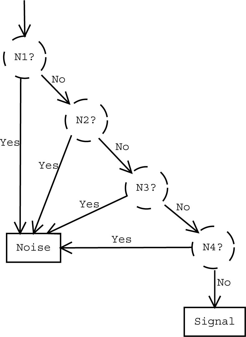
The structure of GDT. The element classifier N1 (resp. N2,N3,N4) evaluates the element discriminant function J1(f) (J2(f), J3(f), J4(f)) returning TRUE if the component pair with the feature vector f is assigned to the noise class 1 (class 2, class 3, class 4). The element discriminant functions are given in Table 2.
To classify a component pair (t, c) with a feature vector f = [f1, . . . , f6]T, the GDT classifier computes the value of the discriminant function J(f). The discriminant function J(f) returns either TRUE ((t, c) is noise related) or FALSE ((t, c) is signal related). The discriminant function J is defined with the help of the element discriminant functions J1, J2, J3, J4, each corresponding to a specific noise class:
| (5) |
where θj are parameter vectors to be learned during the classifier training and denotes the logical OR operation. The element discriminant functions Jj(f|θj) return TRUE if (t, c) belongs to the noise class j and FALSE otherwise. The specific forms of element discriminant functions are given in Table 2.
Table 2.
Discriminant functions for the element classifiers. Λ is the logical AND operation.
|
J1(f|θ1) = (f2 < θ12) Λ (f4 < θ14) Λ (f6 < θ16) |
|
J2(f|θ2) = (f1 < θ21) Λ ((f4 < θ24) (f3 < θ23)) |
|
J3(f|θ3) = (f2 < θ32) Λ (f4 < θ34) Λ (f6 < θ36) |
| J4(f|θ4) = (f4 < θ42) Λ (f4 < θ44) Λ (f5 < θ45) |
2.5.2 Classifier training
It remains to be explained how the parameter vectors θ1, θ2, θ3, θ4 are learned based on the hand-labeled training data. In the Neyman-Pearson framework, we search for the parameter vector estimates that maximize the probability of detection under the constraint that the probability of false alarm is smaller than a given Neyman Pearson (NP) threshold α.
Let denote the set the component pairs hand-classified to the signal class. Let denote the set of component pairs hand-classified to the noise classes that were introduced in Section 2.3. We write . In addition, we define functions
| (6) |
| (7) |
| (8) |
| (9) |
These functions, respectively, return the percentage of the components classified correctly as the noise type j by the element classifier j, classified correctly as noise (detection rate), classified incorrectly as the noise type j by the element classifier j, and classified incorrectly as noise (false alarm rate). Based on these definitions, the GDT training problem can be stated as
| (10) |
where θα = {θ1, θ2, θ3, θ4 : F A(θ1, θ2, θ3, θ4) < α}.
The algorithm for solving (10) is based on the divide and conquer principle and exhaustive search. We start by training the optimal element classifiers, in the Neyman Pearson sense as above, for different candidate thresholds αa for a = 1, . . . , A. That is, we compute
| (11) |
for a = 1, . . . , A, j = 1, 2, 3, 4. Note that for training the element classifier j, the training data only from and are utilized. Then, for all four tuples
we evaluate and to find the complete set of parameters for the GDT classifier according to Eq. (10). An exhaustive search algorithm for solving (11) is sketched in Appendix B.
3 Experiments and results
3.1 Training and test sets
We used two separate data-sets for the validation. The first dataset, referred to as the training set, was used exclusively for training the classifier and validating the classifier structure. The second set, referred to as the test set, was used for validating the classifier trained using the training set. With these data, we compared the results of our automatic classifier to the hand-labeling of the independent component pairs.
For the classifier training, the fMRI data was collected from 20 subjects performing a category learning task. Each acquisition was divided into 6 runs from which 4 were based on the blocked design and 2 were based on the event related design. Imaging was performed with a 3T Siemens Allegra head-only MR scanner. The images were collected using a gradient-echo echo-planar pulse sequence with interleaved acquisition (TR=2000ms, TE=30ms, 64 × 64 matrix, 3.125mm × 3.125mm pixel size, 25 slices, 4mm slice thickness/1mm gap, 200mm FOV). Four images at the beginning of each run were discarded to allow T1 equilibration. The behavioral task and the image acquisition parameters are fully described in (Aron et al., 2006).
Prior to performing ICA, the images were subjected to the standard preprocessing using the FSL software package, including Gaussian spatial smoothing, temporal high-pass filtering, motion correction using FSL's McFlirt (Jenkinsson and Smith, 2001; Jenkinson et al., 2002) and brain extraction using BSE (Smith, 2002). After performing ICA, the resulting component pairs (5321 in total) were hand-labeled as either noise/artifact related or not clearly artifactual as described in Sect. 2.3. The hand labeling was performed by A.R.R. and S.T in consultation with R.P. Thereafter, the component pairs classified as noise were classified into distinct noise classes according to the decision rule in Appendix A. The classifier was trained using these training data as described in Sect. 2.5. The classifiers were trained separately for the event-related and the blocked design cases. Classifiers were trained for NP-thresholds of 0.05, 0.075, 0.10, 0.125, 0.15, 0.175, and 0.2.
The test set, which was not used during the classifier training, contained fMRI data from 12 subjects (Foerde et al., 2006). For each subject, there were 5 runs based on blocked design: a tone counting run, 2 weather prediction runs, and 2 dual task (weather prediction and tone counting) runs. After the weather prediction runs, an event-related probe run was completed. The complete details of the behavioral procedure can be found in (Foerde et al., 2006). The imaging procedure and the applied pre-processing were identical to those with the training set except the images had 30 slices. The component pairs identified by ICA were classified by the GDT classifier and hand-labeled by K.F. for validation purposes.
3.2 Validity of features and classifier structure
We performed area under receiver operating characteristic (ROC) curve (AUC) analysis to validate the pre-determined structure of the GDT classifier (Hanley and McNeil, 1982). Our purpose with this analysis is to provide evidence that the selected three features (among the total six features) for separating each noise class from the signal class are the optimal ones. In our case, it is important that the features for each element classifier provide independent information 2 and they each have good discrimination power between a certain noise class and the signal class. AUC is a measure of the discriminative ability of a test (Hanley and McNeil, 1982). Given two sets of scalar (feature) values, here values from a signal set and a noise set, AUC can be seen as an estimate of the probability that a random value from the signal set is greater than a random value from the noise set. Generally, the higher the AUC the more useful the feature is for discriminating between a certain noise class and the signal class. For computing AUCs, we used a non-parametric procedure based on numerical integration.
The results are listed in Tables 3 and 4. Features f1 and f2 characterizing the power spectrum of the component timecourse are expected to correlate strongly and therefore they ought not to be used in the same element classifier.
Table 3.
AUCs for the blocked design. AUCs for features applied for a particular noise class are in boldface.
| f1 | f2 | f3 | f4 | f5 | f6 | |
|---|---|---|---|---|---|---|
| Class 1 | 0.6305 | 0.7494 | 0.4795 | 0.7012 | 0.5257 | 0.6798 |
| Class 2 | 0.9547 | 0.7971 | 0.8267 | 0.6133 | 0.6168 | 0.2242 |
| Class 3 | 0.5580 | 0.8891 | 0.4916 | 0.6660 | 0.1450 | 0.9448 |
| Class 4 | 0.6580 | 0.6986 | 0.6868 | 0.8820 | 0.9694 | 0.6414 |
Table 4.
AUCs for event related design. AUCs for features applied for a particular noise class are in boldface.
| f1 | f2 | f3 | f4 | f5 | f6 | |
|---|---|---|---|---|---|---|
| Class 1 | 0.8053 | 0.8281 | 0.5741 | 0.7077 | 0.4386 | 0.5164 |
| Class 2 | 0.9372 | 0.8396 | 0.8412 | 0.5891 | 0.6440 | 0.1285 |
| Class 3 | 0.4963 | 0.9313 | 0.5309 | 0.6742 | 0.0994 | 0.9468 |
| Class 4 | 0.8137 | 0.7588 | 0.6642 | 0.8133 | 0.9564 | 0.4816 |
Thus, the selected features for each element classifier were optimal in the sense that they were the three (admissible) features with the highest AUCs with three exceptions. These exceptions are discussed next.
For the noise class 1 in the event related case, feature f3 had a higher AUC than feature f6. The low AUC for f6 might mean that f6 was not good in characterizing noise class 1 in the event related case. However, ROC increased rather rapidly in the beginning and the feature had AUC clearly over 0.5 in the blocked design case. For these reasons, we decided to use it also in the event related case.
For the noise class 2, feature f5 received a higher AUC than feature f4. Feature f4 is meant to discriminate only a part of the noise class 2 from the signal class, and it functions as an alternative to feature f3. That is, we require that either (but not both) f4 or f3 need to have a low value in order for the component pair to be classified to the noise class 2. For this reason, the low AUC of f4 is not particularly worrying and there is no apparent reason to favor f5 over it.
In the event related case and for the noise class 4, feature f1 had higher AUC than feature f2. The feature f1 was found to correlate negatively with both features f4 and f5 when only the noise class 4 in the event related case was studied. For this reason and for the symmetry between blocked and event related design, feature f2 was preferred.
Based on these discussions, we can conclude that the AUC analysis supported the use of the proposed classifier structure.
3.3 Classification performance
We studied the performance of the classifier against manual component classification. We trained the classifiers with multiple NP thresholds (0.05, 0.075, 0.10, 0.125, 0.15, 0.175 and 0.20) using the training set. These classifiers were then used to classify the component pairs in the test set and these classifications were compared to the results of the component pair classification by an expert. The expert (K.F.) was different from the ones who classified the data in the training set. As quantitative indicators of the classifier performance, we computed the false alarm rate (the percentage of component pairs classified as signal by the expert which were classified as noise by the automatic classifier), the miss rate (the percentage of component pairs classified as noise by the expert which were classified as signal by the automatic classifier) and the total misclassification rate (the percentage of the component pairs classified differently by the expert and automatic classifier). The misclassification rate is a weighted average of the false alarm and miss rates.
The results are shown in Fig. 3. As can be seen in Fig. 3, the misclassification rate was always between 0.214 and 0.261. This indicates that the automatic classification and the manual classification were in agreement in general. The misclassification rate was consistent between different NP thresholds. This indicates that the effect of the selecting between different NP thresholds was essentially selecting between different levels of conservativeness of the classification. The false alarm rate in the test set was well in the line with the original NP threshold. This is pleasing because it is important that the selected NP threshold predicts the false alarm rate of the classifier allowing the user to predict the effect of tuning the NP threshold. The miss rates varied between 0.615 and 0.380 with blocked design and 0.746 and 0.438 with event related design. Particularly for the event related design, the classifier with the lowest NP threshold can be too conservative and higher NP thresholds than 0.05 should be preferred.
Fig. 3.

The test errors between manual and automatic classifications
We compared the classification performance on the test set to the training and cross-validation based errors on the training set to obtain information about how differences in the behavioral tasks and manual classification affect the classification performance. The training error refers to the classification error with the same training set as the classifier was trained with. The cross-validation was performed by the leave one out method. We trained the classifiers using the training data from 19 of 20 subjects in training set. The data from the left-out subject was then used to evaluate the classifier. This was repeated 20 times, leaving each subject's data once out of the training set. The leave-one-out error was the pooled error from the 20 repetitions.
The misclassification rate with the test set (test error) is compared to the training and cross-validation (leave-one-out) errors with the training set in Fig. 4. The value of the training error was the lowest and the test error was the highest as expected. However, the difference between the training error and the test error was always below 0.10 indicating that the simple classifier structure indeed led to good generalization ability. The leave-one-out error was very close to the training error (difference was always below 0.04). This indicates that a notable part of the difference between the training and test errors was due to the differences in the manual classifications with the training and test sets and differences in the data of the training set and test set. This could reflect slight differences in the tasks between the studies, or could reflect variability in the application of the manual classification heuristics across the different experts. An interesting observation is that, with the event related design, both training and test errors were at minimum when the NP threshold was 0.1. However, in the blocked design case, there was no such consensus.
Fig. 4.

The misclassification rate with the training set (training error), with the test set (test error) and leave-one-out cross-validated test error with the training set.
3.4 Effects of the size of the training set
We studied if the training set size could be reduced for a more effective classifier training. We applied a bootstrapping strategy to study this (see Efron and Tibshirani (1986)). First, we draw (with replacement) a set of N < 20 subjects form the training set comprising the data of 20 subjects. We trained a classifier with the data of the N randomly selected subjects. Then, the classifier was evaluated with the test-set. This was repeated 100 times for each N and NP-threshold. The average false-alarm and misclassification rates from 100 bootstrap samples were computed as well as standard deviations of these. In Figure 5, the results of these experiments are shown for N = 2, 5 and 10 and the blocked design. Thus, the training sets were comprised of the data from 8,20 and 40 runs. These experiments were performed only on the blocked design data.
Fig. 5.

Average misclassification rates and false alarm rates across the 100 bootstrap runs with different training set sizes. Standard deviations (STD) of misclassification rates and false alarm rates across the 100 bootstrap runs. N = 20 refers to the full training set and it is included as reference. No bootstrapping was performed for N = 20.
The average misclassification rates were almost independent on the size of the training set. The standard deviation of the misclassification rates decreased slowly with increased N. However, the decrease was not notable. Instead, the standard deviation of false alarm rate decreased considerably from the N = 2 case to the N = 10 case. For N = 5 and N = 10, there were only small differences in standard deviations of false alarm rate when NP threshold was small. Therefore, we conclude that the main benefit from having a large training set was that the false alarm rate of the classifier became predictable. Instead, the misclassification rate was not dependent on the size of the training set. Thus, it appears that the classifier can be trained with a considerably smaller training set than the one containing data from 20 subjects if the deviations in false alarm rate are not considered catastrophic.
3.5 Numbers of ICA components
The average numbers of the total ICA components and rejected components for the test set are listed in Table 5. Table 5 also provides the average percentage of rejected components for each run. As expected the number of rejected components increased with the NP threshold. The number of rejected components was somewhat higher in the blocked design case, especially in the percentual level. This indicates that the classification in the event-related case was slightly more conservative than in the blocked design case, as was observed also in Section 3.3.
Table 5.
Numbers of components in the test set for blocked design and event related (ER) design. M is the PPCA estimate of the number of sources for the original 4-D time-series, R is the number rejected components (i.e. those labeled as noise), Mdn is the PPCA estimate of the number of components in the denoised 4-D time-series.
| Blocked design | ER design | |||||||
|---|---|---|---|---|---|---|---|---|
| NP | 0.05 | 0.1 | 0.15 | 0.2 | 0.05 | 0.1 | 0.15 | 0.2 |
| mean M | 43.5 | 43.5 | 43.5 | 43.5 | 51.3 | 51.3 | 51.3 | 51.3 |
| mean R | 7.92 | 11.3 | 12.7 | 14.3 | 4.58 | 9.83 | 12.3 | 14.42 |
| mean R/M | 0.181 | 0.260 | 0.294 | 0.331 | 0.089 | 0.192 | 0.241 | 0.281 |
| mean Mdn | 37.1 | 34.2 | 33.0 | 31.5 | 47.1 | 42.8 | 40.5 | 38.7 |
| mean |Mdn — (M — R)| | 1.60 | 2.01 | 2.17 | 2.23 | 0.67 | 1.50 | 1.50 | 1.75 |
We re-ran PPCA with the denoised datasets to see if the dimensionality estimates before and after denoising were in line. Intuitively, if the original estimate of number of sources was M then the number of sources after the denoising should be M − R, where R is the number noise components. The average of numbers of sources estimated based on denoised data and mean absolute difference between the re-estimated number of sources (Mdn) and M − R are displayed in Table 5. The estimates Mdn were in line with their predicted values M − R (absolute difference was 0 or 1 in 48% of the cases). When the two numbers differed, Mdn were in all cases higher than M − R. The higher Mdn (i.e. more non-Gaussian components than M − R) suggests that the estimated amount of the white Gaussian noise was smaller in the denoised 4-D time-series than in the original 4-D time-series although we did not try explicitly to remove it. This could be an indication that sometimes there were ’hidden’ independent components that were revealed only when the overlaying structured noise was reduced. To pursue this issue further, we re-performed the pICA and classified the components for those denoised 4-D time-series which had larger Mdn (by the margin of 4) than the predicted M − R. The number of these denoised time-series varied from 2 to 4 (of 72 the total runs in the test set) with increased NP threshold . When classifying the IC pairs in ICA decomposition of the denoised data, it turned out that few new noise components were found. However, the number of these was considerably lower than noise components detected in the first round of denoising. Therefore, iterating pICA and denoising would probably have only marginal effect on average but might be useful in some cases.
3.6 Reproducibility across ICA runs
The pICA algorithm used in this study is a stochastic gradient descent algorithm as are most practical ICA algorithms. This means that there is random component in the algorithm (in our case the initialization is randomized) and the results of different ICA runs could be different (see (Himberg et al., 2004) for a more complete account of the reliability of stochastic ICA algorithms). For this reason, we decided to study the effects of this random variation to the denoising results. We re-ran ICA for the test set, performed the denoising for the second run, and studied the differences of the results between the denoising results between the two ICA runs. We note that repeating the procedure only twice does not allow a rigorous evaluation of reliability of our classification procedure with respect to the stochasticity of ICA. However, the complete reliability analysis is beyond the scope of this work.
Most component pairs in the re-run had a rather close counterpart in the original ICA run. However, there were typically some component pairs in the re-run which did not have a matching counterpart in the original run 3. This demonstrates that the ICA results of different runs differed slightly that must be accounted for. Interestingly, those component pairs not having a well matching counterpart in the other run were often those that were differently classified by the classifiers with different NP thresholds.
It is not reasonable to compare the automatic classification of the re-run to the manual classification of the original run, because the component pairs are essentially different. Instead, we considered the effect on the session level and on the group level. To examine the group level effect, we first created a difference image by subtracting the denoised datasets across two ICA runs, computed the average difference timecourse, and took the absolute value of each timecourse value. These were then averaged across the subjects, separately for blocked and event related designs. We also performed an analogous analyses between the original and denoised dataset. On the session (run) level, we computed the Euclidean distances between the corresponding 1-D voxel timecourses of the denoised datasets. These were then divided by the number of time points (T) in the timecourse. From these, we located the maximum for each session and averaged them over all sessions and subjects pooling also the two-design types to the same measure. Again, we performed an analogous analyses between the original and denoised dataset.
On the group level, differences between denoised datasets were negligibly small as compared to differences between the denoised and original datasets. For example, the average (maximum) of the described difference timecourse between the two denoised datasets was 0.000001 (0.000004) for the NP-threshold of 0.2 for both blocked and event related designs. The average (maximum) of the described difference timecourse between the original and denoised dataset was 3.04 (132.5) for the blocked design and 3.02 (166.2) for the event related design. This shows that, on the group level, the denoising method was not sensitive to the stochasticity of pICA. Not surprisingly, on the session level, there appeared to be more differences across two runs. For NP threshold of 0.2, the average maximum distance was 3.09 between denoised datasets while the average maximum distance was 57.8 between the original and the denoised dataset. Hence, on the session level, the maximal distances between the corresponding voxel timecourses in the two denoising runs were approximately 5% of the corresponding distances between the original and denoised datasets. However, when accounting for all voxel timecourses and sessions, these differences between denoising runs were averaged out as was visible from the group level differences.
3.7 Effects of denoising to statistical analysis
3.7.1 Simulation study
3.7.1.1 Data
We performed a simulation to study the effects of denoising to single subject GLM analysis quantitatively. The simulation was built upon a resting state fMRI BOLD scan. An activation pattern modeling the categorization task was then added to the resting state scan. The simulated activation was thus completely known, which made it possible to study the effects of the denoising to the activated regions vs. to the non-activated regions.
The resting state data was obtained from the FBIRN traveling subjects database (http://www.nbirn.net, http://www-calit2.nbirn.net/bdr/fbirn_phase1/index.shtm). We used the first scan of the subject 103 acquired at 3T at the Massachusetts General Hospital (MGH). The scan consisted of 85 time points. The images were collected using a gradient-echo echo-planar pulse sequence with interleaved acquisition (TR=3000ms, TE=40ms, 64 × 64 matrix, 3.4375mm × 3.4375mm pixel size, 35 slices, 4mm slice thickness/1mm gap, 220mm FOV).
The simulated activation time course (blocked design, 18s of rest followed by 18 s of activation modeled by the boxcar function convolved with a haemodynamic response function (HRF)) was added to a set of regions that are generally activated during categorization tasks (caudate, putamen, globus pallidus, thalamus, orbital,lateral and medial frontal cortex) (Aron et al., 2006)). The ROIs were extracted by registering the BOLD scan to a T2-weighted anatomical scan of the subject, and thereafter registering the T2-weighted scan to the T2-weighted single subject BrainWeb image (Collins et al., 1998). All the affine 12-parameter registrations were carried out for skull-stripped images using FSL's Flirt tool (Jenkinsson and Smith, 2001). Anatomical ROIs were obtained using the AAL atlas (Tzourio-Mazoyer et al., 2002); ROIs extracted this way exhibit some degree of anatomical inaccuracy, but this is not a concern for the present simulation. The amplitude of the activation was selected so that the relative effect size was 0.5. The effect size is defined as the ratio of the difference in means between the experimental and control condition and the standard deviation of the noise (Desmond and Glover, 2002). The noise standard deviation was computed over the putatively activated regions as in (Desmond and Glover, 2002). After the addition of the simulated activation to the data, we simulated motion effects of different magnitudes by rotating the 3-D images around the inferior-superior (z) axis using the center of the image as the origin. These rotations were applied at three time points, which were randomly selected. The rotations always took place in the middle of the acquisition of the 3-D image, thus affecting odd and even image planes differently due to the interleaved acquisition. The magnitudes of these rotations were 0 (no movement), 3 (movement 1), and 6 (movement 2) degrees. Preprocessing, ICA, automatic component classification, and denoising were performed as with the training and test sets.
3.7.1.2 GLM analyses
Preprocessing and statistical analysis of the data were performed using the FSL software library (FMRIB, Oxford University, (Smith et al., 2004)). Images were temporally high-pass filtered with a cutoff period of 72 s. Spatial smoothing was applied with a Gaussian kernel with FWHM of 5 mm. Following pre-processing, statistical analyses were performed using the GLM within FSL (FEAT, FMRI Expert Analysis Tool, Smith et al. (2004); Woolrich et al. (2001)). The design matrix contained the timecourse of the simulated activation along with its temporal derivative.
3.7.1.3 Results
We studied how the ROC curves of Z-scores (of contrast between the baseline and the task) were affected by denoising. The ROC curve is a plot of the sensitivity versus false alarm rate of the statistical test. Here, the sensitivity is defined as the percentage of the activated voxels whose Z-scores (under the GLM) exceeded a threshold. The false alarm rate is the percentage of the voxels that were not activated whose Z-scores exceeded the same threshold. We considered only voxels within the brain mask. Note that the ROC curves are independent of the method used to threshold the Z-scores. The ROC curves are presented in Fig. 6. The AUCs (Hanley and McNeil, 1982) for different NP-thresholds are given in Table 6. The ROC curves when no extra movement was simulated were almost identical with different levels of denoising and without denoising. As very high AUCs indicate, the GLM framework was extremely powerful to detect activations at this effect size when the activation was not masked by artifacts. The AUC of the GLM without denoising decreased to 0.9258 and 0.8547 as the magnitude of the simulated movement increased, despite the application of motion correction using MCFLIRT. As can be seen in Fig. 6 and in Table 6, the ICA based denoising markedly improved the discrimination power of GLM resulting in AUCs above 0.94. The ROC curves of the denoised data were above the ROC curve without denoising for all false alarm rates. This shows that denoising improved the final test no matter how the detection thresholds were chosen. The ROC curves for different NP thresholds were almost identical. Also, the Z-scores in activated areas increased over 40% (movement magnitude 1) and 80% (movement magnitude 2) after denoising. This indicates that denoising can improve the activation detection by removing obvious artifacts which could mask the activations.
Fig. 6.

ROC curves of the Z-scores with denoising (NP threshold 0.2) and without denoising. ROC curves for the other NP thresholds were highly similar than the one with the NP threshold 0.2.
Table 6.
AUCs of the Z-scores in the simulation study for different movement magnitudes (γ) in degrees and with and without denoising (the column No DeN).
| γ | No DeN | NP threshold | |||
|---|---|---|---|---|---|
| |
|
0.05 |
0.10 |
0.15 |
0.20 |
| 0 | 0.9735 | 0.9747 | 0.9745 | 0.9745 | 0.9758 |
| 3 | 0.9258 | 0.9680 | 0.9680 | 0.9680 | 0.9680 |
| 6 | 0.8547 | 0.9452 | 0.9452 | 0.9452 | 0.9452 |
It is interesting to take a further look at the ICA components that were rejected by the automatic classifier. The estimated number of ICA components was 44 when there was no simulated movement. From these, a single component pair was rejected by all classifiers with different NP thresholds. The correlation coefficient of the timecourse of the component and the reference function was −0.169, which made it as the 11th most task related component of the total 44. The component map showed a focal region of high intensity in the temporal white matter area and no significant intensities were in the activated regions. The estimated number of ICA components dropped to 7 when the simulated movement effect was added to the data. From these 4 components could be attributed to the simulated motion, and the classifiers with all NP thresholds were able to distinguish these as artifactual (see Fig. 7). The rest of the components were not easily categorized as signal nor noise, and these were all classified to the signal class by the automatic classifiers. The maximum absolute correlation coefficients with the reference function were 0.204 (magnitude 1) and 0.169 (magnitude 2).
Fig. 7.
An example of the ICA timecourse that was related to simulated motion. Prominent increases and decreases in the timecourse corresponded to the occurrences of the simulated motions.
3.7.2 Effects of denoising to group level analyses with the test set
3.7.2.1 Group level analyses
With the test set, we studied the effects of the denoising to the group level analysis. Preprocessing and statistical analysis of the data were performed using the FSL software library (FMRIB, Oxford University, (Smith et al., 2004)) as described by Foerde et al. (2006). Each (motion-corrected) fMR timeseries was denoised as described above, thus creating the denoised dataset. The original dataset refers to the same dataset without denoising.
Images were temporally high-pass filtered with a cutoff period of 75 s for the blocked design data and 66 s for the event-related data. Spatial smoothing was applied with a Gaussian kernel with FWHM of 5 mm. Following preprocessing, statistical analyses were performed at the single-subject level using the general linear model within FSL (FEAT, FMRI Expert Analysis Tool, Smith et al. (2004); Woolrich et al. (2001)). Each event was modeled as an impulse convolved with a canonical HRF (a double gamma function modeling the HRF rise and following undershoot) along with its temporal derivative. For the event-related probe run, trials with correct responses for each task were modeled separately. Specific comparisons of interest were tested using linear contrasts. Following analysis at the individual level, the results were spatially normalized to the MNI-152 template using FSL's FLIRT registration tool (Jenkinsson and Smith, 2001). Functional images were first aligned to the co-planar high-resolution T2-weighted image of the same subject, then the co-planar image was aligned to T1-weighted MP-RAGE image of the same subject, and finally the MP-RAGE image to the standard MNI-152 template. All transformations were carried out using affine transforms with 12 degrees of freedom. Mixed-effects group analyses were performed for each contrast using FSL's FLAME (FMRIB's Local Analysis of Mixed Effects, Beckmann et al. (2003)) module . Higher-level statistical maps were thresholded using clusters determined by Z > 2.3 and a (corrected) cluster significance threshold of P = 0.05 according to the theory of Gaussian random fields (Friston et al., 1994).
3.7.2.2 Results
We compared the effects of the denoising to the white matter (WM) and gray matter (GM) voxels. The WM (GM) were defined as those which were WM (GM) voxels with probability greater than 0.5 in the MNI template. The assumption was that the true activations should occur only in GM. We studied each condition separately. The conditions were: a blocked design single task (blocked-ST), a blocked design dual task (blocked-DT), an event related design single task (ERST) and an event related design dual task (ERDT). In following, Z-scores refer to the Z-scores of the contrast between the baseline and the task.
The differences (averaged over GM and WM voxels) of the group-level Z-scores between the denoised and original data are displayed in Fig. 8. Not surprisingly, the denoising reduced Z-scores on average and this decrease was greater when the NP-threshold was increased. The decrease for the white matter was greater than the decrease for the gray matter. This suggests that denoising worked as intended: it reduced more the Z-scores in the areas (WM) where high Z-scores are likely to be due to imaging artifacts than in the areas (GM) where high Z-scores also reflect true activations. (Hence, the Z-score reduction in GM is harder to intepret than the Z-score reduction in WM). Examples of images displaying areas where the Z-scores were increased or decreased by at least 0.33 in the BDDT condition are shown in Figs. 9. As expected, the higher the NP threshold the more voxels were affected by denoising. This pattern was even more prominent with other conditions, especially with the event related conditions. With the BDDT condition, the regions where Z-scores decreased were mostly in WM regions. Prominent increases of the Z-scores were observed in the thalamus and in regions of the ventral frontal and temporal cortex near areas of susceptibility artifact. These regions could be plausibly involved in learning on the basis of feedback (which is the nature of the task used here) (O'Doherty et al., 2003). This suggests that the present technique may be particularly useful for enhancing detection of fMRI signals in regions near areas of susceptibility artifacts.
Fig. 8.

Average Z-score difference (original - denoised) in GM and WM as a function of the NP threshold.
Fig. 9.
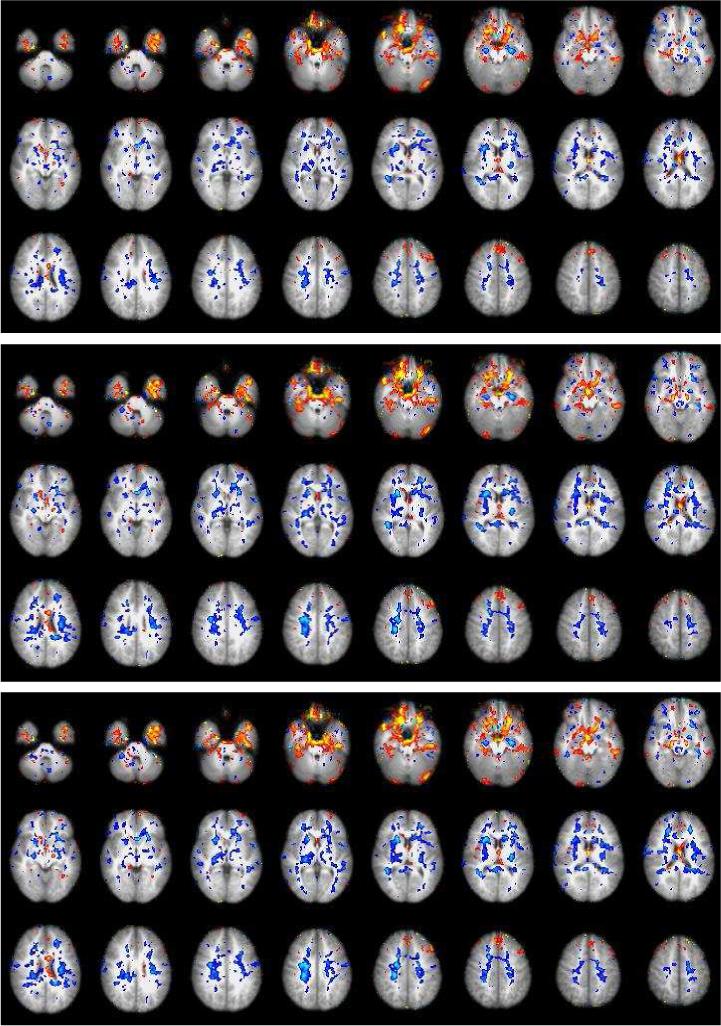
Voxel locations where the Z-score increased (red/yellow) or decreased (blue/white) by denoising with the blocked-DT condition. The NP-thresholds from top are 0.05, 0.10 and 0.15.
We additionally compared the difference in parameter estimates between the original and the denoised datasets as a function of the parameter estimate in the original dataset. The figure 10 shows examples of these plots with the dual task conditions when the NP threshold was 0.15. The plots with the other NP thresholds were consistent with these. As it can be seen in Fig. 10, the denoising decreased the absolute value of the signal (i.e. increased negative signal values and decreased positive signal values). Thus, the overall effect of the denoising procedure is a shrinkage of parameter estimates towards zero. This adds to the evidence that the denoising works as intended, however, this should not be taken as a figure of merit in itself.
Fig. 10.

Average signal difference between the original and filtered datasets as function of the signal level in the original data. Left: Blocked DT-condition, right: ERDT condition.
We studied whether the ICA-based denoising affected the group analysis comparing the blocked-ST and the blocked-DT conditions, which was one of the main interests in (Foerde et al., 2006). On visual inspection of the group analysis results, the differences between the original and denoised data appeared marginal, with the results based on denoised data generally having fewer significant voxels and missing some small clusters (see Fig. 11 for an example). This is encouraging, since our aim was to reduce the effect of fMRI artifacts to gain more accurate and robust activity detection.
Fig. 11.
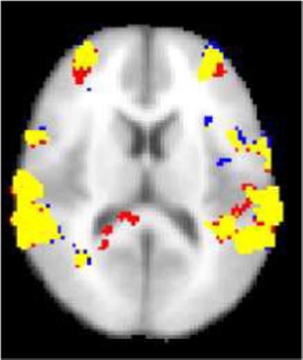
An axial slice of the map showing regions of the greater dual task activity than single task activity in the group analysis (significance threshold P = 0.05, whole-brain corrected using Gaussian Random Field Theory). Yellow: The voxel is activated both for the denoised dataset and the original dataset. Red: The voxel is activated only for the original dataset. Blue: The voxel is activated only for the denoised dataset. The main effect of denoising was the reduction of the activations detected in white matter posterior to the ventricles. The NP threshold was 0.05.
4 Discussion
We have described and evaluated a method for automatic identification of the artifact related independent components (ICs) in BOLD fMRI. These ICs related to artifacts were then rejected from the data providing a denoised dataset. Our denoising method was based on supervised classification using global Neyman-Pearson decision trees. In supervised classification, the classifier parameters are learned from the training data. In this case, the training data consisted of independent component pairs classified by an expert as either potentially artifactual (noise) or not clearly artifactual (signal). To facilitate the classification of an independent component pair, we generated a set of six features characterizing different aspects of the pair. These features related to the component timecourse, the power spectrum of component timecourse, and the spatial structure of the component map. The use of spatial aspects of component maps is a novel feature among the algorithms aimed to classification of the independent component pairs. In other contexts, it has been demonstrated that certain motion related fMRI artifacts can be well characterized by particular patterns in the component maps (McKeown et al., 1998, 2003; Liao et al., 2006).
The global decision tree classifier was chosen for a number of reasons. 1) The global decision trees lead to simple and easily controllable classifier structures (i.e. decision regions have simple shapes). Given a relatively small training set whose labeling can be subjective, this can be considered preferable as long as the classifier can explain the training set well enough. Still, the shape of the decision regions can be complex enough that our classifier can identify most of the component pairs reflecting fMRI artifacts. 2) The global decision tree can be designed to agree well to the hand-labeling procedure. This can be considered important as long as we rely on the hand-labeling procedure and the supervised classification framework. 3) The Neyman-Pearson framework allowed us to introduce an user controllable conservativeness parameter. This may reduce the need for additional training to implement the classification under novel behavioral tasks or image acquisition procedures. 4) Adaptations of the classifier structure are easy to implement by adding additional features to the classifier. Also, if a particular type of noise would be especially prominent, the objective function for the classifier training can be modified to account for this. In our framework, it is straight forward to introduce weights to the training data characterizing how important it is to classify a certain training sample correctly. 5) Finally, in our case, the probability density functions (pdfs) of feature values in different classes are not known and in general they are not easily estimated; thus, we can not consider classifiers relying on the known parametric families for the class pdfs.
As mentioned, the user must set the level of conservativeness of denoising by tuning the NP threshold. It could be tempting to select the NP threshold that minimizes the mis-classification rate with the training set (training error). However, the value of this strategy is questionable. Firstly, as indicated in Section 3, the best training error was achieved with a different NP threshold than the best test error in the blocked design case. The test error can be considered as the ultimate performance measure of the classification. Hence, the threshold that minimizes the training error may not be the optimal NP threshold for test data. Secondly, the test and the training errors are both computed with respect to the manual classification, which is subjective and not perfectly reliable. A better idea would be to select the NP threshold with respect to group level analysis results. Here, we have demonstrated the effects of denoising with different NP thresholds to the group level analysis with category learning tasks. It was demonstrated with these tests that tuning the NP threshold indeed affects the level of conservativeness of the denoising in a rather predictable manner. However, these experiments did not identify a principled way to the select the optimal threshold. The optimal threshold likely varies with the imaging protocol and and paradigm design. We plan to address this problem in a future work with the aim to select maximal NP threshold which does not impair the detection of true activation in the group analysis.
We have evaluated our classifier/denoising scheme with the fMRI data from category learning tasks. The evaluation consisted of three parts. First, we studied whether the features modeled what they were designed to model and whether the classifier structure was suitable. This was achieved by performing a separate ROC analysis for each feature and for each noise class. Both the classifier structure and the features were found to be appropriate. Second, we evaluated the classification performance against the manual component pair classification. This is important because the manual identification of clearly artifact related independent components and their subsequent removal from the data have been previously recommended (FEAT User guide http://www.fmrib.ox.ac.uk/fsl/feat5/detail.html). Finally, we have demonstrated the effects of the denoising on the group level statistical analysis. These effects (e.g. reduced Z-scores in white matter) were similar as expected which can be considered as evidence that the denoising truly works as intended, though we would recommend that investigators perform similar validation to that presented here before using the present methods with paradigms that differ substantially from those used here. The reduction in Z-score values in WM is not important in itself as WM voxels could be masked out - these kind of anatomical constraints can be embedded already to ICA (Formisano et al., 2004). Instead, the reduction serves as an indication that the artifacts were reduced also in gray matter areas of the brain as we did not utilize GM/WM decomposition in our algorithm. We performed also a simulation study to quantify the effects of denoising to the GLM-based statistical analysis. In the simulation, we placed a simulated activation corresponding to a categorization task and simulated movement artifacts on top of resting state fMRI time-course. The ICA based denoising was able to identify the residual movement artifacts after movement correction and consequently improved the activation detection under GLM. It must be stressed that, although we aimed at a realistic simulation, in reality the BOLD-signal increases and movements do not take place after all the noise from the other sources already exist in the data, but the different noise processes and activation related BOLD increases affect the data simultaneously. Thus, the simulation of realistic fMRI data presents a huge challenge. Further work is required to completely understand the effects of denoising to GLM/GRF group level analyses and, although our classifier is presented in this context, its application is not limited to denoising for GLM/GRF based analyses.
ICA has been applied within fMRI for numerous applications (see McKeown et al. (2003) for a review) and there are some works not directly related to the denoising application, but which are nevertheless interesting from the perspectives of this study. Liao et al. (2005, 2006) studied the minimization of head motion induced variations in fMRI by coupling ICA and motion correction. This way they were able to reduce interpolation artifacts and correct for simulated between slice motions. While the joint ICA and motion correction (MCICA) approach aims to reduce the effect of partially same artifacts than our denoising approach, the approaches are different. Whereas our approach identifies and models the noise components, the MCICA approach builds on the knowledge of the true activation and, as discussed in (Liao et al., 2006), reduces to the ordinary, multivariate mutual information based motion correction when such knowledge is not available. Also, as (Liao et al., 2005) discussed, MCICA methodology may require extensions before more local deformations such as cardiac and respiratory pulsation could be corrected for by it. However, it might be that our classification scheme combined with MCICA (i.e. MCICA instead of the gross head motion correction by McFlirt) would lead to improved detection of fMRI artifacts. In a recent article, De Martino et al. (2007) introduced IC-fingerprints for characterizing independent components and used support vector machines to classify them into six classes including activation and noise classes. Their methodology was based on the supervised classification and some of our features have counterparts in their IC fingerprints (particularly our features f1, f2, f6). Also, some IC fingerprints were derived based on spatial organization of the component map values as were our features f3 and f4. However, these IC fingerprints were different from f3 and f4. The work of De Martino et al. (2007) was not directly aimed at the denoising application - although it might well be possible to apply their classifier for denoising purposes. This slightly different focus from ours relates to the selection of the classifier. For us, as explained previously, it is important to control the false alarm rate of the classifier and that the decision regions of the classifier are simple. Thus, we prefer global decision trees under the NP framework instead of, for example, support vector machines. However, we wish to note that a Neyman-Pearson implementation of support vector machines was recently proposed by Davenport et al. (2006).
Acknowledgments
This work was supported by the Academy of Finland under the grants 204782, 108517, 104834 and 213462 (Finnish Centre of Excellence program (2006-2011)), the National Science Foundation through grants NSF BCS-0223843 and NSF DMI-0433693 to R.P, and the National Institutes of Health through the NIH Roadmap for Medical Research, grant U54 RR021813 entitled Center for Computational Biology (CCB). Information on the National Centers for Biomedical Computing can be obtained from http://nihroadmap.nih.gov/bioinformatics. Additional support was provided by the NIH/NCRR resource grant P41 RR013642.
Appendix A: The decision rule
We describe the decision rule for assigning a component pair with the feature vector f = [f1, . . . , f6]T into one of the noise classes. Again, we consider blocked and event related designs separately. For j = 1, . . . , 6, let nj denote the number of those feature vectors in the signal class in the training data which have greater value of the feature j than is the total number of the feature vectors in the signal class. Then the decision rule is
Appendix B: Solving the element classifier parameters
We formulate the classifier training algorithm for the case where the discriminant function is of the form
For the other cases, the formulation is highly similar. The aim is to find the parameters which maximize the detection rate of the element classifier (Dj(θj) in Eq. (6)) under the constraint that (see Eq. (8)). We have the manually labeled training samples from the noise class j and from the signal class . The algorithm is as follows:
Let
for l = 1, 2, 3.
Find such , that
Here ∊ is a small positive constant. can be found by evaluating all the possibilities
Denote by (a, b] the half-open interval between the scalars a and b. Because Dj(θj) is constant in all regions
where , it is enough to evaluate it once in each region. Also, within this region, F Aj(θj) is the smallest when θj = [f1[k1] + ∊, f2[k2] + ∊, f3[k3] + ∊]T if ∊ is small enough.
This algorithm can be accelerated using variety of techniques. Also, because the algorithm tabulates Dj(θj) and F Aj(θj) for each θj in the lookup table with no additional computation cost, it is possible to find the classifier for several NP thresholds simultaneously.
Footnotes
Publisher's Disclaimer: This is a PDF file of an unedited manuscript that has been accepted for publication. As a service to our customers we are providing this early version of the manuscript. The manuscript will undergo copyediting, typesetting, and review of the resulting proof before it is published in its final citable form. Please note that during the production process errors may be discovered which could affect the content, and all legal disclaimers that apply to the journal pertain.
We performed also a correlation analysis between the features for each element classifier. The results were as expected and therefore they are not presented.
To automatically find the best matching component pair in another ICA run, we correlated a component timecourse in the original run with each component time-course in the re-run and the studied the maximum absolute value of the correlation coefficients. If the maximum was low, then we could say that there was no match. Note that 1) it is sufficient to study only the component timecourses as component maps are computed based on these and the original image series; 2) ’the maximum of correlation coefficients’ analysis is immune to the ambiguities of ICA.
References
- Aron A, Gluck M, Poldrack R. Long-term test-retest reliability of functional mri in a classification learning task. NeuroImage. 2006;29(3):1000–1006. doi: 10.1016/j.neuroimage.2005.08.010. [DOI] [PMC free article] [PubMed] [Google Scholar]
- Beauchamp M. Detection of eye movements from fMRI data. Magn. Res. Med. 2003;49:376–380. doi: 10.1002/mrm.10345. [DOI] [PubMed] [Google Scholar]
- Beckmann C, Jenkinson M, Smith S. General multi-level linear modelling for group analysis in fmri. NeuroImage. 2003;20:1052–1063. doi: 10.1016/S1053-8119(03)00435-X. [DOI] [PubMed] [Google Scholar]
- Beckmann C, Smith S. Probabilistic independent component analysis for functional magnetic resonance imaging. IEEE Trans Med Imaging. 2004;23(2):137–152. doi: 10.1109/TMI.2003.822821. [DOI] [PubMed] [Google Scholar]
- Bennett K. Global tree optimization: A non-greedy decision tree algorithm. Computing Science and Statistics. 1994;26:156–160. [Google Scholar]
- Bennett K, Blue J. Tech. Rep. Math Report 214. Rensselaer Polytechnic Institute; Troy, New York, USA: 1996. Optimal decision trees. [Google Scholar]
- Biswal B, DeYoe A, Hyde J. Reduction of physiological fluctuations in fmri using digital filters. Magn Reson Med. 1996;35:107–113. doi: 10.1002/mrm.1910350114. [DOI] [PubMed] [Google Scholar]
- Breiman L, Friedman J, Stone C, Olshen R. Classification and Regression Trees. Taylor and Francis; 1984. [Google Scholar]
- Collins L, Zijdenbos A, Kollokian V, Sled J, Kabani N, Holmes C, Evans A. Design and construction of a realistic digital brain phantom. IEEE Trans Med Imag. 1998;17(3):463–468. doi: 10.1109/42.712135. [DOI] [PubMed] [Google Scholar]
- Davenport MA, Baraniuk RG, Scott CD. Controlling false alarms with support vector machines; IEEE International Conference on Acoustics, Speech, and Signal Processing (ICASSP06)..2006. pp. 589–592. [Google Scholar]
- De Martino F, Gentile F, Esposito F, Balsi M, Di Salle F, Goebel R, Formisano E. Classification of fMRI independent components using IC-fingerprints and support vector machines. NeuroImage. 2007;34:177–194. doi: 10.1016/j.neuroimage.2006.08.041. [DOI] [PubMed] [Google Scholar]
- Desmond JE, Glover GH. Estimating sample size in functional mri (fmri) neuroimaging studies: statistical power analyses. J Neurosci Methods. 2002 Aug;118(2):115–128. doi: 10.1016/s0165-0270(02)00121-8. [DOI] [PubMed] [Google Scholar]
- Diedrichsen J, Shadmehr R. Detecting and adjusting for artifacts in fmri time series data. NeuroImage. 2005;27:624–634. doi: 10.1016/j.neuroimage.2005.04.039. [DOI] [PMC free article] [PubMed] [Google Scholar]
- Duda RO, Hart PE, Stork DG. Pattern Classification, 2nd Edition. Wiley-Interscience; New York: 2001. [Google Scholar]
- Efron B, Tibshirani R. Bootstrap methods for standard errors, confidence intervals, and other methods of statistical accuraciest. Stat. Sci. 1986;1:54–75. [Google Scholar]
- Foerde K, Knowlton B, Poldrack R. Modulation of competing memory systems by distraction. Proc Nat Acad Sci. 2006;103:11778–11783. doi: 10.1073/pnas.0602659103. [DOI] [PMC free article] [PubMed] [Google Scholar]
- Formisano E, Esposito F, DiSalle F, Goebel R. Cortex-based independent component analysis of fMRI time series. Magn. Reson. Imaging. 2004;22:1493–1504. doi: 10.1016/j.mri.2004.10.020. [DOI] [PubMed] [Google Scholar]
- Frackowiak RSJ, Friston KJ, Frith CD, Dolan RJ, Price C, Zeki S, Ashburner J, Penny W, editors. Human Brain Function. 2nd edition. Academic Press; 2003. [Google Scholar]
- Freire L, Mangin J-F. Motion correction algorithms may create spurious brain activations in the absence of subject motion. NeuroImage. 2001;14:709–722. doi: 10.1006/nimg.2001.0869. [DOI] [PubMed] [Google Scholar]
- Freire L, Roche A, Mangin J-F. What is the best similarity measure for motion correction in fmri time series. IEEE Trans Med Imaging. 2002;21:470–484. doi: 10.1109/TMI.2002.1009383. [DOI] [PubMed] [Google Scholar]
- Friston K, Williams S, Howard R, Frackowiak R, Turner R. Movement-related effects in fmri time-series. Magn Reson Med. 1996;35:346–355. doi: 10.1002/mrm.1910350312. [DOI] [PubMed] [Google Scholar]
- Friston K, Worsley K, Frakowiak R, Mazziotta J, Evans A. Assessing the significance of focal activations using their spatial extent. Human Brain Mapping. 1994;1:210–221. doi: 10.1002/hbm.460010306. [DOI] [PubMed] [Google Scholar]
- Grootoonk S, Hutton C, Ashburner J, Howseman A, Josephs O, Rees G, Friston K, Turner R. Characterization and correction of interpolation effects in the realignment of fmri time series. NeuroImage. 2000;11:49–57. doi: 10.1006/nimg.1999.0515. [DOI] [PubMed] [Google Scholar]
- Hanley J, McNeil B. The meaning and use of the area under a receiver operating characteristic (roc) curve. Radiology. 1982;143:29–37. doi: 10.1148/radiology.143.1.7063747. [DOI] [PubMed] [Google Scholar]
- Himberg J, Hyvärinen A, Esposito F. Validating the independent components of neuroimaging time-series via clustering and visualization. NeuroImage. 2004;22(3):1214–1222. doi: 10.1016/j.neuroimage.2004.03.027. [DOI] [PubMed] [Google Scholar]
- Hyvärinen A, Oja E. Independent component analysis: Algorithms and applications. Neural Networks. 2000;13:411–430. doi: 10.1016/s0893-6080(00)00026-5. [DOI] [PubMed] [Google Scholar]
- Jenkinson M, Bannister P, Brady J, Smith S. Improved optimisation for the robust and accurate linear registration and motion correction of brain images. NeuroImage. 2002;17:825–841. doi: 10.1016/s1053-8119(02)91132-8. [DOI] [PubMed] [Google Scholar]
- Jenkinsson M, Smith S. A global optimisation method for robust affine registration of brain images. Medical Image Analysis. 2001:143–156. doi: 10.1016/s1361-8415(01)00036-6. [DOI] [PubMed] [Google Scholar]
- Kochiyama T, Morita T, Okada T, Yonekura Y, Matsumura M, Sadato N. Removing the effects of task-related motion using independent-component analysis. NeuroImage. 2005;25(3):802–814. doi: 10.1016/j.neuroimage.2004.12.027. [DOI] [PubMed] [Google Scholar]
- Kruger G, Glover G. Physiological noise in oxygenation-sensitive magnetic resonance imaging. Magn Reson Med. 2001;46:631–637. doi: 10.1002/mrm.1240. [DOI] [PubMed] [Google Scholar]
- Liao R, Krolik J, McKeown M. An information-theoretic criterion for intrasubject alignment of fmri time series: Motion corrected independent component analysis. IEEE Trans Med Imag. 2005;24(1):29–44. doi: 10.1109/tmi.2004.837791. [DOI] [PubMed] [Google Scholar]
- Liao R, McKeown M, Krolik J. Isolation and minimization of head-motion induced signal variations in fMRI data using independent component analysis. Magn. Reson. Med. 2006;55:1396–1413. doi: 10.1002/mrm.20893. [DOI] [PubMed] [Google Scholar]
- Lund TE, Madsen KH, Sidaros K, Luo W-L, Nichols TE. Non-white noise in fmri: does modelling have an impact? Neuroimage. 2006 Jan;29(1):54–66. doi: 10.1016/j.neuroimage.2005.07.005. URL http://dx.doi.org/10.1016/j.neuroimage.2005.07.005. [DOI] [PubMed]
- McKeown M. Detection of consistently task-related activation in fmri data with hybrid independent component analysis. NeuroImage. 2000;11:24–35. doi: 10.1006/nimg.1999.0518. [DOI] [PubMed] [Google Scholar]
- McKeown M, Hansen L, Sejnowski T. Independent component analysis of functional mri: what is signal and what is noise? Curr Opin Neurobiol. 2003;13(5):620–629. doi: 10.1016/j.conb.2003.09.012. [DOI] [PMC free article] [PubMed] [Google Scholar]
- McKeown M, Makeig S, Brown G, Jung T, Kindermann S, Bell A, Sejnowski T. Analysis of fMRI data by blind separation into independent spatial components. Human Brain Mapping. 1998;6:160–188. doi: 10.1002/(SICI)1097-0193(1998)6:3<160::AID-HBM5>3.0.CO;2-1. [DOI] [PMC free article] [PubMed] [Google Scholar]
- Moritz C, Rogers B, Meyerand M. Power spectrum ranked independent component analysis of a periodic fmri complex motor paradigm. Human Brain Mapping. 2003;18(2):111–122. doi: 10.1002/hbm.10081. [DOI] [PMC free article] [PubMed] [Google Scholar]
- O'Doherty J, Critchley H, Deichmann R, Dolan R. Dissociating valence of outcome from behavioural control in human orbital and ventral prefrontal cortex. J. NeuroSci. 2003;23(21):7931–7939. doi: 10.1523/JNEUROSCI.23-21-07931.2003. [DOI] [PMC free article] [PubMed] [Google Scholar]
- Perlbarg V, Bellec P, Anton J, Pelegrini-Issac M, Doyon J, Benali H. CORSICA: correction of structured noise in fMRI by automatic identification of ICA components. Magn Reson Imaging. 2007;27(1):35–46. doi: 10.1016/j.mri.2006.09.042. [DOI] [PubMed] [Google Scholar]
- Petersson KM, Nichols TE, Poline JB, Holmes AP. Statistical limitations in functional neuroimaging. i. non-inferential methods and statistical models. Philos Trans R Soc Lond B Biol Sci. 1999 Jul;354(1387):1239–1260. doi: 10.1098/rstb.1999.0477. URL http://dx.doi.org/10.1098/rstb.1999.0477. [DOI] [PMC free article] [PubMed]
- Quinlan JR. C4.5: Programs for machine learning.; Morgan Kauffmann. 1993. [Google Scholar]
- Rao CR. A decomposition theorem for vector variables with a linear structure. Ann. Math. Statist. 1969;40(5):1845–1849. [Google Scholar]
- Salli E, Korvennoja A, Visa A, Katila T, Aronen H. Reproducibility of fMRI: Effect of the use of contextual information. NeuroImage. 2001;13:459–471. doi: 10.1006/nimg.2000.0702. [DOI] [PubMed] [Google Scholar]
- Smith S. Fast robust automated brain extraction. Human Brain Mapping. 2002;17:143–155. doi: 10.1002/hbm.10062. [DOI] [PMC free article] [PubMed] [Google Scholar]
- Smith S, Jenkinson M, Woolrich M, Beckmann C, Behrens T, Johansen-Berg H, Bannister P, Luca MD, Drobnjak I, Flitney D, Niazy R, Saunders J, Vickers J, Zhang Y, Stefano ND, Brady J, Matthews P. Advances in functional and structural mr image analysis and implementation as fsl. Neuroimage. 2004;23(S1):208–219. doi: 10.1016/j.neuroimage.2004.07.051. [DOI] [PubMed] [Google Scholar]
- Stoica P, Moses R. Introduction to Spectral Analysis. Prentice-Hall; Englewood Cliffs, NJ: 1997. [Google Scholar]
- Thomas CG, Harshman RA, Menon RS. Noise reduction in BOLD-based fMRI using component analysis. NeuroImage. 2002;17(3):1521–1537. doi: 10.1006/nimg.2002.1200. [DOI] [PubMed] [Google Scholar]
- Tipping M, Bishop C. Probabilistic principal component analysis. (Series B 61).J R Stat Soc. 1999:611–622. [Google Scholar]
- Tzourio-Mazoyer N, Landeau B, Papathanassiou D, Crivello F, Etard O, Delcroix N, Mazoyer B, Joliot M. Automated anatomical labeling of activations in spm using a macroscopic anatomical parcellation of the mni mri single-subject brain. Neuroimage. 2002 Jan;15(1):273–289. doi: 10.1006/nimg.2001.0978. URL http://dx.doi.org/10.1006/nimg.2001.0978. [DOI] [PubMed]
- Woolrich M, Ripley B, Brady J, Smith S. Temporal autocorrelation in univariate linear modelling of fmri data. NeuroImage. 2001;14:1370–1386. doi: 10.1006/nimg.2001.0931. [DOI] [PubMed] [Google Scholar]
- Wu D, Lewin J, Duerk J. Inadequacy of motion correction algorithms in functional MRI: role of susceptibility-induced artifacts. Magn Reson Imaging. 1997;7:365–370. doi: 10.1002/jmri.1880070219. [DOI] [PubMed] [Google Scholar]