An Electrostatic Deformable Model for Medical Image Segmentation

Abstract

A new deformable model, the charged fluid model (CFM), that uses the simulation of charged elements was used to segment medical images. Poisson's equation was used to guide the evolution of the CFM in two steps. In the first step, the elements of the charged fluid were distributed along the propagating interface until electrostatic equilibrium was achieved. In the second step, the propagating front of the charged fluid was deformed in response to the image gradient. The CFM provided sub-pixel precision, required only one parameter setting, and required no prior knowledge of the anatomy of the segmented object. The characteristics of the CFM were compared to existing deformable models using CT and MR images. The results indicate that the CFM is a promising approach for the segmentation of anatomic structures in a wide variety of medical images across different modalities.

1 INTRODUCTION

Image segmentation is a fundamental problem in computer graphics and medical image processing. It is one of the most important steps in imaging-based analyses requiring feature extraction, image measurements, shape representation or other forms of image understanding [1–3]. The principal goal of the segmentation process is to partition an image into several regions of interest such that each region has similar characteristics of gray-level and texture. Segmentation methods for monochrome images can be classified into several categories including pixel-based [3], edge-based [4,5], region-based [2,6], knowledge-based [7,8] approaches and deformable models [9,10]. Some of the most popular and successful methods are deformable models due to their ability to accurately recover the shape of biological structures in many medical image segmentation applications [11,12].

Deformable models involve the formulation of a propagating interface, which is a closed curve in 2-D or a closed surface in 3-D, that is moving under a speed function determined by local, global and independent properties [13]. Given the initial position of a propagating interface and the corresponding speed function, deformable models track the evolution of the interface during the segmentation process. Existing deformable models can be broadly divided into two categories: parametric and geometric.

Parametric deformable models, originating from the active contour model introduced by Kass et al. [14], explicitly represent the interface as parameterized contours in a Lagrangian framework. Active contour models use an energy-minimizing spline that is guided by internal and external energies in such a way that the deformation of the spline is restricted by geometric shape forces and influenced by image forces. By optimizing the weights used in the internal energy and choosing the proper image forces (e.g., lines or edges), active contour models can be used to evolve the curve toward the boundaries of objects being segmented. Cohen [15] extended active contour methods such that the curve behaves like a balloon to obtain more stable results.

One of the disadvantages of parametric deformable models is the difficulty of naturally handling topological changes for the splitting and merging of contours. This problem is readily solved by geometric deformable models when implemented using the level set numerical algorithm developed by Osher and Sethian [16]. The principle underlying level set methods is to adopt an Eulerian approach that implicitly models the propagating interface using a level set function φ, whose zero-level set always corresponds to the position of the interface [13]. The evolution of this propagating interface is governed by a partial differential equation in one higher dimension. The level set function can be constructed with high accuracy in space and time. The position of the zero-level set is evolved using a speed function that consists of a constant term and a curvature deformation in its normal direction [16].

Caselles et al. [17] and Malladi et al. [18] proposed a geometric deformable contour with an image gradient stopping force based upon the Osher-Sethian level set framework,

$$\frac{\partial \phi }{\partial t}=g(I)(V_0+\epsilon \kappa )|\hspace{0.17em}\nabla \phi \hspace{0.17em}|$$ (1)

where V₀ and ε are constant weights, κ is the level set curvature, ∇ is the gradient operator, and g(I) is the stopping force based upon the image gradient given as

$$g\left(I\right)=\frac{1}{1+{|\hspace{0.17em}\nabla G_{\sigma }\ast I\left(x,y\right)\hspace{0.17em}|}^p}$$

where G_σ is a Gaussian filter with standard deviation σ, I(x, y) is a given 2-D image and p = 1 or 2. In the above equation, * represents convolution and | · | is the modulus of the smoothed image gradients.

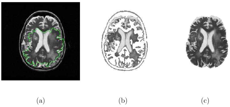
The Caselles-Malladi deformable contour notably improved the initialization of parametric active contours provided that the initial contour was placed symmetrically with respect to the boundaries of interest [12,13]. In practice, this is not easy to achieve since many medical image segmentation problems are not dealing with regularly shaped objects. Fig. 1 demonstrates the difficulty of using the Caselles-Malladi deformable contour to segment the brain with convoluted shapes in T2-weighted MR images. Note that the initial contour was not symmetrically placed with respect to the brain. It was not easy to choose an appropriate stopping force required to achieve satisfactory results. The contour was confined inside by the high intensity structures when using a stronger stopping force and the contour leaked past the brain boundaries when using a weaker stopping force [see (1)].

Fig. 1.

Difficulty of using the Caselles-Malladi deformable contour in segmenting the brain in T2-weighted MR images. (a) The initial contour that was not symmetrically placed. (b) The contour was confined inside the brain by the inner high intensity structures using a strong stopping force. (c) Some of the contour were crossed over the brain boundaries while some contours were restricted inside, using a slightly weaker stopping force. (d) The contour leaked past the brain boundaries using a weaker stopping force.

Kichenassamy et al. [19] and Yezzi et al. [20] added a doublet term, ∇g · ∇φ, to (1) to efficiently attract the evolving contour to the desired feature. Siddiqi et al. [21] subsequently modified the speed function by adding a term based upon the gradient flow derived from a weighted area energy functional so that the contour could more flexibly evolve toward the desired edges. Vasilevskiy and Siddiqi [22] proposed a flux maximizing flow method to the segmentation of blood vessels. Goldenberg et al. [23] used a variational geometric framework with coupled surfaces for cortex segmentation. Recently, Gout et al. [24] proposed a segmentation approach that combines the idea of the geodesic active contour and interpolation of points in the Osher-Sethian level set framework to find a boundary contour from a finite set of given points.

Alternatively, Chan and Vese [25] proposed a region-based approach, active contours without edges, based upon level set methods and Mumford-Shah segmentation techniques [26], satisfying the evolution equation

$$\frac{\partial \phi }{\partial t}={\delta }_{\epsilon }(\phi )[\mu \kappa -{\lambda }_1{(I-c_1)}^2+{\lambda }_2{(I-c_2)}^2]$$ (2)

where δ_ε is the Dirac delta function, which is numerically approximated by the Heaviside function H; μ ≥ 0, λ₁ > 0, λ₂ > 0 are fixed parameters, and c₁, c₂ are the averages of I inside and outside the contour respectively. This approach aims to automatically perform 2-phase segmentation of the image I, given by I = c₁H + c₂(1 − H), with interior contours. It can detect objects whose boundaries are not necessarily defined by the image gradient or with very smooth boundaries.

It has been shown that the Chan-Vese active contour is robust to contour initialization in that the initial contour can be anywhere in the image and does not necessarily have to surround the objects being segmented [25]. However, it is difficult to use the Chan-Vese active contour to segment anatomic structures that have an intensity distribution similar to the background as illustrated in Fig. 2. This approach incorrectly captured the brain and divided the image into two distinct regions based upon the intensity values [see (2)]. The authors subsequently extended this model by proposing a multiphase level set framework to segment images with more than two regions [27]. The initialization can be regularly arranged using multiple contours for each level set function. Drapaca et al. [28] modified the Chan-Vese level set framework and extended it to higher dimension segmentation problems. However, these algorithms [27,28] may not converge to a global solution for a given initial condition. Later, Holtzman-Gazit et al. [29] proposed a thin structure segmentation method that combined the Chan-Vese model with the boundary alignment.

Fig. 2.

Difficulty of using the Chan-Vese active contour in segmenting the brain in Fig. 1. (a) The initial contour. (b) to (c) The evolution of the contour. (d) The Chan-Vese method failed to correctly extract the brain in that the darker part of the brain was excluded and the brighter part of the background was included as the segmentation results.

In this paper, we propose a new deformable model, the charged fluid model (CFM), that extends and modifies the charged fluid framework [30] for medical image segmentation. In our earlier study, we used the simulation of a charged fluid governed by Poisson's equation as a deformable model to perform general image segmentation. The evolution consisted of two alternate procedures that were designed to deform the contour in response to the image data. It automatically handled topological changes at the interface and provided sub-pixel precision for the area and length of the segmented region. However, it was not easy to segment complex and difficult anatomic structures in medical images. This paper reports on the extension of the mathematical formulas and modification of the numerical techniques to achieve a more robust segmentation algorithm to extract anatomic structures in medical images. It requires a contour initialization step to start the algorithm, but we will demonstrate that it is less critical than the Caselles-Malladi method. In addition, we compare the results obtained using the CFM to those obtained using the Caselles-Malladi and Chan-Vese methods in segmenting a variety of anatomic structures in medical images. Lastly, the CFM has been extended to 3-D for volumetric segmentation applications.

This paper is organized as follows. In Section 2, we introduce the concept of the charged fluid and present the necessary background on the mathematical model of the charged fluid framework. In Section 3, we describe new mathematical equations and numerical techniques that improve the charged fluid framework. We also present a new segmentation algorithm based upon the CFM. In Section 4, we discuss the unique properties of the CFM in the segmentation of medical images with various modalities, and compare the CFM to the Caselles-Malladi and Chan-Vese methods. We also illustrate the applications of the 3-D CFM to 3-D vascular tree segmentation in 3-D X-ray rotational angiography (3DRA) images. In Section 5, we summarize the results and contributions of the current work.

2 Mathematical Model

We shall start by describing the use of physics-based particle systems for the simulation of deformable models. The concept of using a particle simulation was introduced by Reeves [31] to model objects such as fire, clouds, and water. In his model, particles move under the influence of external forces and constraints without interacting with each other. More recent particle systems use a simulation of molecular dynamics governed by the Lennard-Jones function to add links between the particles to guide the evolution of a deformable model [32,33]. In these elastic particle systems, intensive numerical computation is required to obtain particle attributes such as position, velocity, force, torque, and orientation. We developed the charged fluid method [30] that changed the property and structure of charged particles without the computation of velocity, acceleration and torque. This resulted in a particular characteristic that the charged fluid behaves like a liquid flowing through and around objects. We now briefly review the mathematics underlying the charged fluid method [30].

2.1 Concept

The basic concept is to use a system of charged elements as a deformable model to perform image segmentation. A number of charged elements with the same sign of charge are placed on a propagating interface that is modeled as the surface of an isolated conductor. The fluid elements repel each other due to the electric forces and advance toward an equilibrium state to minimize the electrostatic energy. When electrostatic equilibrium is achieved, each fluid element (the large circles in Fig. 3) has a net charge as if it was calculated by interpolating the charges of the covered particles (the solid dots in Fig. 3). The electric forces (F_ele in Fig. 3) are perpendicular to the contour and their magnitudes are proportional to the charge of the corresponding element. Moreover, the fluid element deforms in response to external forces F_ext (e.g., the image gradient) as illustrated in Fig. 3. This electrostatic system is governed by Poisson's equation

Fig. 3.

Schematic illustrating the concept of a charged fluid. A charged fluid conceptually consists of charged elements (the large circles), each of which exerts a repelling electric force upon the others. The fluid elements behave as if they consisted of different numbers of charged particles (the solid dots). The charged fluid can be influenced by internal repulsive electric forces (F_ele) and external restrictive forces (F_ext) from the image data.

$${\nabla }^2\Phi \left(\text{r}\right)=-4\pi \rho \left(\text{r}\right)$$ (3)

where Φ is the electric potential and ρ(r) is the known charge density. To make use of the simulation of a charged fluid for image segmentation, we evolved the curve using two sequential procedures described below. Herein, we have adopted the notation (x,y) to represent Cartesian coordinates in the spatial domain, (m,n) to represent discrete coordinates in the spatial domain, and (u,v) to represent the corresponding discrete coordinates in the Fourier domain.

2.2 Curve Evolution

The curve evolution of the charged fluid consisted of two procedures that were repeated until the contour resided on the boundaries of objects being segmented. The first procedure, charge distribution, allowed the charged fluid to flow within the propagating interface until a specified electrostatic equilibrium was achieved. The second procedure, front deformation, deformed the propagating front into a new shape in response to the image potential, which was related to the image gradient. During curve evolution, fluid elements were restricted to move on the lattice.

2.2.1 Charge Distribution

In order to handle topological changes when using multiple charged fluids, Poisson's equation in (3) was modified as

$${\nabla }^2{\widehat{\Phi }}_{\text{ele}}={\nabla }^2\sum _j{\widehat{\Phi }}_{\text{ele}}^j=-4\pi \sum _j{\widehat{\rho }}^j=-4\pi \widehat{\rho }$$ (4)

where ${\widehat{\Phi }}_{\text{ele}}$ is the normalized electric potential and $\widehat{\rho }$ is the normalized charge density of the overall system at each time step. In the above equation, ${\widehat{\Phi }}_{\text{ele}}^j$ is the normalized electric potential for the charged fluid j

$${\widehat{\Phi }}_{\text{ele}}^j=\frac{{\Phi }_{\text{ele}}^j}{{\overline{\Phi }}^j}{\Phi }_0$$

where Φ₀ is an arbitrary positive constant and ${\overline{\Phi }}^j$ is the mean electric potential in the charged fluid j. The corresponding normalized charge density, ${\widehat{\rho }}^j$, for the charged fluid j was defined as

$${\widehat{\rho }}^j=\frac{{\rho }^j}{{\overline{\Phi }}^j}{\Phi }_0.$$ (5)

During this procedure, the electric field E_ele in the discrete domain was numerically computed using the central difference approximation of the normalized electric potential in the following equation,

$${\text{E}}_{\text{ele}}=-\nabla {\widehat{\Phi }}_{\text{ele}}.$$ (6)

The advancement distances ${\text{d}}_x^i$ and ${\text{d}}_y^i$ for each fluid element i was then numerically computed as

$$\begin{array}{c}{\text{d}}_x^i=\frac{{\text{E}}_m^i}{E_{\text{max}}}\frac{h}{2}\\ {\text{d}}_y^i=\frac{{\text{E}}_n^i}{E_{\text{max}}}\frac{h}{2}\end{array}$$ (7)

where ${\text{E}}_m^i$ and ${\text{E}}_n^i$ are the electric field components of element i in the m and n axes, respectively. In the above equation, h is the grid spacing and E_max is the magnitude of the maximum electric field on the propagating interface of the system for each iteration. Once the distances were obtained, the fluid element with charge Q was interpolated into adjacent discrete points using the subtracted dipole scheme (SUDS) technique [34]. All fluid elements were continuously advanced until a specified electrostatic equilibrium condition was satisfied using

$$\frac{\Delta Q_{\text{total}}}{Q_{\text{total}}}\le \gamma$$ (8)

where Q_total is the total charge of the overall system for each iteration, ΔQ_total is the net flowing charge in total and γ > 0 determines the degree of electrostatic equilibrium.

2.2.2 Front Deformation

The front deformation procedure allowed the charged fluid to interact with the image data by defining an effective field E_{e f f} as

$${\text{E}}_{\text{e f f}}={\text{E}}_{\text{equ}}+{\text{E}}_{\mathrm{img}}=\nabla {\Phi }_{\text{img}}-\nabla {\widehat{\Phi }}_{\text{equ}}$$ (9)

where E_equ is the electric field in equilibrium corresponding to the normalized electric potential in equilibrium, ${\widehat{\Phi }}_{\text{equ}}$, that was obtained when equilibrium was achieved in the charge distribution procedure and E_img is the image field corresponding to the image gradient potential, Φ_img,

$${\Phi }_{\text{img}}(m,n)=\beta \frac{|\hspace{0.17em}\nabla G_{\sigma }(m,n)\ast I(m,n)\hspace{0.17em}|}{{\hspace{0.17em}|\nabla G_{\sigma }\ast I\hspace{0.17em}|}_{\text{max}}}{\Phi }_0$$ (10)

where β is a weighting factor (β ≥ 0) to adjust the image gradient potential, | · | is the modulus of the smoothed image gradients, and | · |_max is the maximum modulus in the computation domain. The smoothing of the image was performed by convolution with a 3 × 3 or 5 × 5 Gaussian filter kernel.

2.3 Electric Potential Computation

The widely-adopted FSP method [35] was used to solve the electric potential in (4). Given fluid elements having charge Q(m,n) on grid (m,n), we first computed the discrete Fourier transform (DFT) of the charge Q(m,n) using

$$Q(u,v)\equiv \frac{1}{L_m{L}_n}\sum _{m=0}^{L_m-1}\sum _{n=0}^{L_n-1}Q(m,n)exp[\frac{-2\pi \text{ium}}{L_m}]exp[\frac{-2\pi \text{ivn}}{L_n}]$$ (11)

where L_m and L_n are the lengths along the m and n axes, respectively. The electric potential was then computed through Poisson's equation as

$$\Phi (m,n)=\sum _{u=0}^{L_m-1}\sum _{v=0}^{L_n-1}\prime \frac{Q(u,v)}{\pi (\frac{u^2}{L_m^2}+\frac{v^2}{L_n^2})}exp[-2{\pi }^2(\frac{u^2}{L_m^2}+\frac{v^2}{L_n^2})]exp[\frac{2\pi \text{ium}}{L_m}]exp[\frac{2\pi \text{ivn}}{L_n}]$$ (12)

where the prime represents that u = v = 0 is excluded from the sum. The DFT pair in (11) and (12) was rapidly computed using the FFT algorithm provided that L_m = 2^s and L_n = 2^t, where s and t are positive integers.

3 CHARGED FLUID MODEL

In this section, we describe how the mathematical model described in Section 2 was applied to medical image segmentation.

3.1 Mean Electric Field

One problem of using a pure electrostatic model in the charged fluid was that the magnitude of the electric field on each fluid element varies greatly when the geometry of the contour is irregularly shaped. This is due to the fact that the magnitude of the electric field is proportional to the corresponding local charge density [30]. When segmenting noisy images using the charged fluid, those fluid elements that exert a relatively small magnitude electric field will be confined by strong image gradients inside the region during the evolution determined by (9). As a consequence, the contour of the charged fluid may become jagged and the small magnitude inner fluid elements can dramatically retard the convergence speed of the overall system. To address this problem, E_equ in (9) was modified to incorporate the mean magnitude of the electric fields in the charged fluid and rewritten as Ẽ_equ. The magnitude of Ẽ_equ was modified using

$$|\hspace{0.17em}{Ẽ}_{\text{equ}}\hspace{0.17em}|=\text{max}(|\hspace{0.17em}{Ẽ}_{\text{equ}}\hspace{0.17em}|,\langle |\hspace{0.17em}{Ẽ}_{\text{equ}}\hspace{0.17em}|\rangle )$$ (13)

where | · | is the magnitude of Ẽ_equ, 〈·〉 is the mean magnitude of Ẽ_equ on all fluid elements for each charged fluid, and max(·, ·) is the greater of the two values. The result is that the electric strength of weak fluid elements is increased such that the magnitude of the overall electric field in the charged fluid system is uniform, which makes the CFM more robust in segmenting noisy structures in medical images.

3.2 Image Gradient Field

The image gradient potential and the corresponding image field described in Section 2.2 were developed for a general segmentation algorithm regardless of the gray-level of objects and background [30]. In other words, the charged fluid segmented bright objects of interest on dark background, and vice versa, without changing the image potential term in the algorithm. One characteristic of this strategy is that one can obtain particular segmentation results slightly larger or smaller by choosing a proper Gaussian filter and the sign of β in (10). This is due to the use of the second derivative of image intensities, which can be observed by substituting (10) into (9). Nevertheless, taking the gradient of the smoothed image twice can generate a large variation of magnitude along the boundaries of interest. This can sometimes ruin the segmentation results by creating unwanted noise that confines fluid elements inside the region of interest (ROI), when using a large weight of β to prevent leakage. In medical image segmentation applications, it is often desired to directly use the image gradient field to interact with fluid elements such that E_img in (9) is modified as Ẽ_img,

$${Ẽ}_{\text{img}}=\beta {\Phi }_0\frac{\nabla G_{\sigma }(m,n)\ast I(m,n)}{{\left|\hspace{0.17em}\nabla G_{\sigma }\ast I\hspace{0.17em}\right|}_{\text{max}}}.$$ (14)

The effective field E_{e f f} in (9) is correspondingly modified as Ẽ_{e f f},

$${Ẽ}_{\text{e f f}}=\{\begin{array}{l}{Ẽ}_{\text{equ}}+{Ẽ}_{\text{img}}:\hspace{0.17em}\hspace{0.17em}\text{the ROI is darker than background},\hfill \\ {Ẽ}_{\text{equ}}-{Ẽ}_{\text{img}}:\hspace{0.17em}\hspace{0.17em}\text{the ROI is brighter than background}.\hfill \end{array}$$ (15)

Therefore, the CFM is better able to segment anatomic structures with blurred boundaries in medical images.

3.3 Curve Evolution

In this section, we describe new numerical techniques to implement curve evolution in the CFM. For the charge distribution procedure described in Section 2.2.1, we used a uniform charge distribution over the fluid elements that were initially placed on a 2 pixel wide propagating interface obtained in the first procedure as illustrated in Fig. 4(a). The fluid elements were repeatedly advanced inside the charged fluid using the SUDS method until the system converged to an equilibrium state that satisfied (8) as illustrated in Fig. 4(b). Note that the electric fields at the fluid elements are approximately in the normal direction to the contour. We then refined the 2 pixel wide interface to a 1 pixel wide front by boundary element detection.

Fig. 4.

The charge distribution procedure. (a) A uniform charge distribution is used for the fluid elements (the red solid dots) at the beginning of this procedure. They are only allowed to share charge on the 2 pixel wide propagating interface that is obtained from the front deformation procedure (see Fig. 5). The empty charge positions on the interface are represented by the blue hollow circles. (b) The system reaches the equilibrium charge distribution and the electric fields (the arrows) on the elements are approximately perpendicular to the contour. The 1 pixel wide front (not shown) is then obtained by using the boundary element detection technique as described in Section 3.3. Note that the shape of the contour remains the same in this procedure.

This was achieved by using a boolean array corresponding to the image dimension. An initial boolean value was assigned to each corresponding pixel based upon the following rules: true if it was inside the initial contour and false if it was outside. True pixels were reset to the position of the new fluid element during curve evolution. An examination was performed at each time step by checking the boolean values of the 3 × 3 neighboring positions of each element on the 2 pixel wide interface. If the boolean value of any of the 8 neighbors was false, the fluid element was treated as a boundary element, which constituted the 1 pixel wide front. If the boolean values of all neighbors were true, the fluid element was treated as an inner element and discarded. Using this simple technique, the 1 pixel wide front was quickly constructed and the fluid elements were connected by 4-connectivity as illustrated in Fig. 5(a). The front deformation was executed on each fluid element by locating binary positions corresponding to the four adjacent grid points based upon the effective field direction as illustrated in Fig. 6. The 2 pixel wide binary interface was then generated as illustrated in Fig. 5(b) and the CFM evolved into a different shape in response to the effective field in (15).

Fig. 5.

The front deformation procedure. (a) After the charge distribution procedure, the fluid elements are on a 1 pixel wide front with 4-connectivity. Note that the tiny inner charges in Fig. 4(b) are discarded after boundary element detection. The effective fields (the arrows) are computed using the electric field in equilibrium and the image field. (b) A new 2 pixel wide propagating interface is obtained by locating the four adjacent grid points according to the effective field direction shown in (a) for each element based upon Fig. 6. Note that, compared to Fig. 4(a), the propagating interface evolves into a different shape in response to the effective fields.

Fig. 6.

Schematic illustrating the localization of a 2 pixel wide binary interface on an individual fluid element. (a) The effective field E_{e f f} on a fluid element (the red solid dot). (b) The four adjacent grid points (the blue hollow circles) of the element are generated according to the effective field direction in (a) and denoted as a part of the 2 pixel wide propagating interface.

3.4 Segmentation Algorithm

There are two effective parameters in the CFM algorithm: γ in (8) and β in (14). For medical image segmentation, the value of the parameter γ was suggested to be within the range of 1% to 10%. We therefore set the value of γ to 3% for all of the medical image segmentation experiments. The appropriate value of β is discussed in Section 4. The value of ${\overline{\Phi }}^j$ in (5) was initially set to Φ₀ at the beginning of the evolution. Some trivial constants in the CFM were set as follows: Φ₀ = 10, 000 in (14) and h = 1 in (7). Note that multi-resolution scheme can be obtained by setting different values for the grid spacing h. Coarse grid scales can be used at beginning to accelerate the evolving speed for advancing the contour toward the ROI, where tiny grid sizes can then be used for refinement.

The algorithm was terminated when the number of the fluid elements on the 1 pixel wide front [see Fig. 5(a)] remained equivalent for two consecutive steps, i.e., there was no deformation in the charged fluid shape after one more iteration. After the evolution was terminated, a ROI extraction procedure was performed on the entire image using a standard contour tracing algorithm [36]. The software was developed in Java using the UCLA jViewBox [37] for image I/O, display and manipulation. The pseudocode for the CFM algorithm is summarized in Algorithm 1, which consists of two core algorithms corresponding to the charge distribution procedure and the front deformation procedure, respectively.

Algorithm 1: Charged fluid

1. parameter setting of β in (14)

2. image field computation using (14)

3. repeat(i)

   1. uniform charge distribution over fluid elements

   2. repeat(j)

      Algorithm 2

   3. until(j) electrostatic equilibrium is achieved by setting γ = 3% in (8)

   4. 1 pixel wide front construction using the boundary element detection method

   5. Algorithm 3

   6. mean potential computation and charge normalization using (5)

4. until(i) no deformation in the charged fluid shape

5. ROI extraction

6. sub-pixel precision calculation, if desired

Algorithm 2: Charge distribution procedure

1. forward FFT computation of the charge array based upon (11)

2. inverse FFT computation of the potential array based upon (12)

3. electric field computation using (6)

4. advance distance computation using (7)

5. charge interpolation using the SUDS

Algorithm 3: Front deformation procedure

1. mean electric field compensation using (13)

2. effective field computation using (15)

3. 2 pixel wide interface localization based upon Fig. 6

3.5 Computational Complexity

The charge distribution procedure (Algorithm 2) dominated the overall computational cost of the charged fluid algorithm. Using an FFT-based FSP algorithm changed the computational complexity from approximately O(N²), with N equal to the number of particles, to O(M²logM), where M is the length of the square that is used for the electric potential computation provided that L_m = L_n = M [see (11) and (12)]. Most parametric deformable models have complexity O(m), with m equal to the number of nodes. Since the level set framework added one extra dimension to the problem [16], early deformable models have complexity O(n³) in 3-D with n equal to the number of grid points in the spatial direction [13]. The more efficient narrow-band implementation technique has computational complexity O(kn²), with k equal to the number of cells in the narrow band.

4 RESULTS AND DISCUSSION

The results of using the CFM algorithm to segment magnetic resonance (MR) and computed tomography (CT) images were compared to the results obtained using the Caselles-Malladi and Chan-Vese methods. We used a variety of medical images that have dimension 256 × 256 for MR and 512 × 512 for CT. Since there were no clear stopping criteria for the Caselles-Malladi and Chan-Vese algorithms, the results were obtained after a steady state was observed by inspection, unless stated otherwise. In order to quantitatively evaluate our approach, we defined an overall pixel-based measure, conformity κ_c,

$${\kappa }_c\equiv (1-\frac{F_P+F_N}{T_P})\times 100\%$$

where F_P represents false positives, F_N represents false negatives, and T_P represents true positives of the segmentation results. All measures were based upon manual segmentation results by experts for each experiment.

4.1 Topological Changes

We first demonstrate the behavior of the CFM in handling topological changes in a free 2-D space using multiple charged fluid contours, i.e., β = 0 in (14). Fig. 7(a) shows three square contours initialized in a free plane, two of which were crossed by each other. In Fig. 7(b), the two contours automatically merged to one at the next iteration based upon the numerical implementation of curve evolution described in Section 3.3. The charged fluids are treated as independent systems when they are not touching each other, and the contours retain the same geometry and topology while they are evolving in a free space as shown in Fig. 7(c). However, the fluid elements from one charged fluid not only interact with themselves but also with those from the other charged fluid when they are close and merging as demonstrated in Fig. 7(d). Finally, Figs. 7(e) and 7(f) show the merged propagating front of the CFM preserving the same topology after further evolution.

Fig. 7.

Evolution of the CFM contours in a free 2-D space. (a) Initialization of three charged fluids using square contours, two of which were crossed by each other. (b) The two contours merged to one after one iteration. (c) The contours kept the same geometry while evolving. They were treated as independent systems when they were away without touching each other. (d) The fluid elements from one charged fluid not only interacted with themselves but also with those from the other when merging. (e) The remaining contour after merging. (f) The contour preserved the same topology after further evolution.

Fig. 8 illustrate the curve evolution of the CFM with β = 8.0 in a phantom image having 6 asymmetrical lobes with simulated cortex from the Internet Brain Segmentation Repository (IBSR) [38]. Two 4 × 4 square contours were separately initialized in the simulated cortex as shown in Fig. 8(a). The contours then deformed in response to the shape of the cortex while approaching each other as depicted in Fig. 8(b) to 8(d). In Fig. 8(e) the two contours were merged into one that was further split into two contours with one inside the other as shown in Fig. 8(f).

Fig. 8.

Curve evolution of the CFM contours in a phantom image of 6 asymmetrical lobes with simulated cortex from the IBSR. (a) Initialization of the CFM using two 4 × 4 square contours. (b) and (c) The contours were constrained evolving in the simulated cortex structure. (d) The evolving contours before merging. (e) The two contours merged together while evolving. (f) The merged contour split into two separated contours with one inside the other.

4.2 Sensitivity Analysis of Initialization and Parameter β

We investigated the ability of the CFM algorithm to segment the brain in Fig. 1 with the initial contour placed accordingly as illustrated in Fig. 9(a). The CFM contour then evolved toward the boundaries of the brain and flowed around inner high intensity structures as shown in Figs. 9(b) and 9(c). Using β = 0.8, the CFM successfully captured the brain with conformity κ_c = 98.36% as illustrated in Fig. 9(d).

Fig. 9.

Experimental results on the effect of CFM initialization in segmenting the brain in Fig. 1. (a) The initial contour was placed corresponding to that in Figs. 1 and 2. (b) and (c) The evolution of the contour. (d) The segmentation results with conformity κ_c = 98.36% using β = 0.8.

We also studied the sensitivity and robustness of the CFM to the parameter β, which is related to the position of the maximum gradient magnitude of an image [see (14)]. Fig. 10 shows the performance of the CFM in segmenting brain tumors in T2-weighted MR images using different values of β. The selection of β is usually set close to unity, however, if the position of the maximum gradient is outside the ROI, then a larger value of β is required. A normalized image gradient map can be used to facilitate the procedure of finding an appropriate value of β for the ROI. As illustrated in Figs. 10(b) and 10(c), the contours leaked from where there are relatively weaker boundary gradients when using relatively lower values of β. The segmentation results were approximately the same using β = 2.0 to 18.0 as shown in Fig. 10(d) to 10(f). The results were deteriorated when using higher values of β as illustrated in Figs. 10(g) and 10(h). The performance measures are summarized in Table 1.

Fig. 10.

Sensitivity analysis of the parameter β in segmenting brain tumors in T2-weighted MR images. (a) The initial contour used in all experiments. (b) and (c) The contours leaked through weak boundaries using lower values of β = 1.2 and β = 1.6. (d) The result with κ_c = 86.32% using β = 2.0. (e) The result with κ_c = 90.12% using β = 10.0. (f) The result with κ_c = 90.48% using β = 18.0. (g) and (h) The results were the same (κ_c = 66.67%) using β = 19.0 and β = 30.0.

Table 1.

Performance measures of the results in Fig. 10 for the sensitivity analysis of the parameter β in segmenting brain tumors.

Image	Parameter β	Conformity κc
Fig. 10(d)	2.0	86.32%
Fig. 10(e)	10.0	90.12%
Fig. 10(f)	18.0	90.48%
Fig. 10(g)	19.0	66.67%
Fig. 10(h)	30.0	66.67%

4.3 Segmentation of Medical Images

4.3.1 2-D Anatomic Structure Segmentation

In this section, we illustrate the segmentation results of the Chan-Vese, Caselles-Malladi and CFM methods using a variety of MR and CT images. The results of using these techniques to segment brain tumors in T2-weighted MR images are illustrated in Figs. 11 and 12. Note that the tumor in Fig. 11 is connected to the ventricle that has a similar intensity distribution, and the tumor in Fig. 12 is surrounded by brain tissue that has close intensity values. The Chan-Vese method almost captured the tumor in Fig. 11 during curve evolution when other anatomic structures were also segmented [indicated by the arrow in Fig. 11(c)]. It was difficult to stop the algorithm at this stage since a steady state was not observed. In the experiments illustrated in Fig. 12, the Chan-Vese contour leaked through the boundaries of the tumor while some of interest regions were not segmented as shown in Fig. 12(b). Finally, the Chan-Vese algorithm respectively separated the images into two regions based upon the intensity distribution as illustrated in Figs. 11(e) and 12(e).

Fig. 11.

Comparison of different segmentation techniques in segmenting the brain tumor in T2-weighted MR images. (a) The initial contour. (b) to (d) The evolution of the contour using the Chan-Vese algorithm. Note that the tumor was almost captured during curve evolution when other anatomic structures were also included as the ROI [indicated by the arrow in (c)]. It was difficult to stop the algorithm during the evolution since a steady state was not observed. (e) The Chan-Vese segmentation result. (f) The result using a simple intensity thresholding. (g) The Caselles-Malladi result (κ_c = 64.21%) using a strong stopping force. (h) The Caselles-Malladi contour was leaking using a slightly weaker stopping force. (i) The result (κ_c = 85.99%) using the CFM with β = 6.0.

Fig. 12.

Using different segmentation techniques to segment the brain tumor in T2-weighted MR images. (a) The initial contour. (b) to (d) The evolution of the Chan-Vese contour. The surrounding tissue has similar intensity to the tumor so that it was difficult to capture the ROI without including other anatomic structures. (e) The Chan-Vese segmentation result. (f) The result using a simple intensity thresholding. (g) The result of the Caselles-Malladi algorithm using a strong stopping force with κ_c = 40.34%. (h) The Caselles-Malladi contour leaked past the boundaries using a slightly weaker stopping force. (i) The result (κ_c = 80.35%) using the CFM with β = 8.0.

Figs. 11(g) and 12(g) illustrate that the contours of the Caselles-Malladi method were confined inside the tumors when a strong stopping force was used. When using a slightly weaker stopping force, the contours leaked past the boundaries of the ROI as depicted in Figs. 11(h) and 12(h), respectively. The results obtained using the CFM algorithm were better than those obtained using the Caselles-Malladi and Chan-Vese methods in that the contour faithfully deformed in response to the shape of the tumors as illustrated in Figs. 11(i) and 12(i).

Fig. 13 illustrates the segmentation results using the Caselles-Malladi, Chan-Vese, and CFM methods in the segmentation of the brain in T2-weighted MR images. It was difficult to use the Caselles-Malladi algorithm to successfully extract the brain due to the convoluted shape of the structures; some parts of the contour leaked past weak boundary gradients while other parts were confined inside as depicted in Fig. 13(a). The Chan-Vese method failed to correctly segment the ROI in that the darker structures of the brain were excluded as shown in Fig. 13(b). The CFM algorithm successfully captured the boundary of the brain (κ_c = 98.72%) as illustrated in Fig. 13(c).

Fig. 13.

Comparison of the segmentation results using different algorithms in extracting the brain in T2-weighted MR images. (a) The result using the Caselles-Malladi method with κ_c = 28.05%. Note that few part of the contour leaked past the boundaries while most stayed inside the ROI. (b) The result using the Chan-Vese method. (c) The result (κ_c = 98.72%) of the CFM using β = 0.5.

We conclude this section by illustrating the ability of the CFM algorithm to successfully segment difficult objects in pulmonary CT images. Figs. 14 and 15 show the results obtained using the Caselles-Malladi, Chan-Vese, and CFM methods for lung segmentation, which is required to identify the lung boundaries within the images. The lung in Fig. 14 has inner high intensity structures (some of which are connected to the lung boundaries) and the lung in Fig. 15 has blurred and ragged boundaries. The Caselles-Malladi contours were confined inside by the lung boundaries using a strong stopping force as depicted in Figs. 14(b) and 15(b). Using a slightly weaker stopping force resulted in leakage as respectively illustrated in Figs. 14(c) and 15(c).

Fig. 14.

Comparison of different segmentation techniques in extracting the lung in pulmonary CT images. (a) The initial contour. (b) The result (κ_c = −27.04%) of the Caselles-Malladi method using a strong stopping force. (c) The Caselles-Malladi contour leaked through the boundaries using a slightly weaker stopping force. (d) The result using the Chan-Vese method. Note that the background, whose intensity is similar to the lung, was also included as the ROI. (e) The result using a simple intensity thresholding. (f) The result using the CFM (β = 1.8) with κ_c = 98.99%.

Fig. 15.

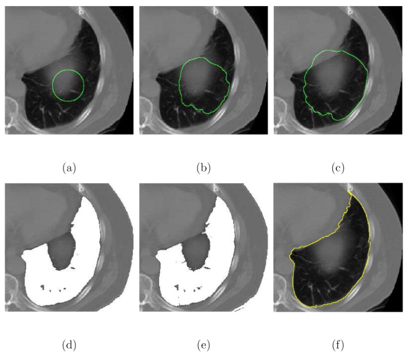
Using different segmentation algorithms to segment the lung in pulmonary CT images. (a) The initial contour. (b) The result (κ_c = −50.61%) of the Caselles-Malladi method using a strong stopping force. (c) The Caselles-Malladi contour leaked past the boundaries using a slightly weaker stopping force. (d) The Chan-Vese method was unable to correctly capture the lung boundary. (e) The result using a simple intensity thresholding. (f) The result (κ_c = 98.02%) of the CFM using β = 1.8.

The Chan-Vese method failed to separate the lungs from the inner structures and the backgrounds as illustrated in Figs. 14(d) and 15(d). The images were incorrectly divided into two regions based upon the intensity values. The Chan-Vese algorithm also failed to exclude the blurred structure illustrated in Fig. 15(d) so that the lung boundaries were not correctly captured. The CFM algorithm successfully extracted the boundaries of the lungs while excluding inner structures and artifacts using a single initial contour with β = 1.8 as shown in Figs. 14(f) and 15(f). Finally, Table 2 summarizes the performance measures of the Caselles-Malladi and CFM methods, and Table 3 shows the approximate computation time using the CFM.

Table 2.

Quantitative analysis of the results obtained using the Caselles-Malladi and CFM methods in segmenting medical images.

Image	κc: Caselles-Malladi	κc: CFM
Fig. 11	64.21%	85.99%
Fig. 12	40.34%	80.35%
Fig. 13	28.05%	98.72%
Fig. 14	−27.04%	98.99%
Fig. 15	−50.61%	98.02%

Table 3.

Computation time using the CFM executed on a Pentium M 1.6 GHz machine running the Windows XP operating system.

Image	Fig. 9	Fig. 10	Fig. 11	Fig. 12	Fig. 13	Fig. 14	Fig. 15
Time	16 s	1 s	4 s	1 s	16 s	192 s	56 s

4.3.2 3-D Vascular Tree Segmentation

In this section, we demonstrate the extension of the 2-D CFM algorithm to higher dimensions in the applications of 3-D vascular tree segmentation. The 3-D CFM algorithm can be constructed based upon the mathematical models and numerical techniques described in Sections 2 and 3. We first demonstrate the evolution of the 3-D CFM algorithm in a vascular-shaped structure as shown in Fig. 16. A 3-D charged fluid started from a small cube in the simulated vessel was used to extract the object as shown in Fig. 16(a). The 3-D charged fluid then evolved toward the boundaries of interest and its shape was changed in response to the geometry of the structure as illustrated in Figs. 16(b) and 16(c), respectively. Finally, in Fig. 16(d), the 3-D charged fluid flowed into the bifurcation structure and segmented the entire vessel.

Fig. 16.

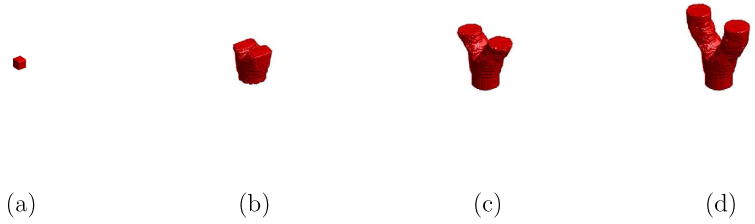
Illustration of segmenting a vascular-shaped structure using the 3-D CFM. (a) The 3-D CFM started from a small cube. (b) and (c) The evolution of the 3-D CFM during the process. (d) The segmentation results.

Using the segmentation strategy illustrated in Fig. 16, we applied the 3-D CFM to segment a number of vascular trees in 3DRA (256 × 256 × 256) images. An initial seed region was manually decided to start the algorithm that automatically segmented the entire vascular trees. Fig. 17 illustrates the 3-D segmentation results of the basilar artery and internal carotid artery structures in different 3DRA image data sets. The 3-D visualization was implemented in the MATLAB ® environment. We show, in Fig. 18, the qualitative comparison of internal carotid artery segmentation results between the 3-D CFM and manual extraction, which has better resolution with local magnification.

Fig. 17.

Experimental results of the 3-D vascular tree segmentation using the 3-D CFM in 3DRA image volumes. (a) and (b) Internal carotid artery structures. (c) Basilar artery structures.

Fig. 18.

Qualitative comparison of internal carotid artery segmentation results using the 3-D CFM and manual extraction in 3DRA images. (a) The result of using the 3-D CFM in a 256 × 256 × 256 image volume. (b) The result of manual segmentation in a 256 × 231 × 256 image volume of the data in (a) locally magnified.

4.4 Discussion

We described a new deformable model, the CFM algorithm, that extends the charged fluid framework presented in our earlier study [30] to segment a variety of medical images. We illustrated the unique properties and essential characteristics of the CFM in handling topological changes and validated its ability in segmenting anatomic structures in medical images without requiring prior knowledge of the underlying anatomy. The CFM is conceptually straightforward, using a two stage curve evolution procedure to achieve contour deformation. The topological changes of the contours are handled by the boundary element detection technique described in Section 3.3 and demonstrated in Figs. 7 and 8. The spirit of the CFM is to rapidly advance the contour toward the boundary of the ROI (pixel by pixel) during the evolution, and then refine the results to the desired precision.

The CFM is capable of capturing objects that have a similar intensity distribution to the background as illustrated in Fig. 9 (see also Figs. 1 and 2). The initial contour of the CFM does not need to be placed at the center with respective to the ROI. We investigated the sensitivity of the CFM to the parameter β in the segmentation of brain tumors as illustrated in Fig. 10. Close segmentation results were obtained using a wide range of β values as summarized in Table 1. We investigated a variety of medical image segmentation applications using brain MR and chest CT images, and compared the results obtained using the CFM to those using the Caselles-Malladi and Chan-Vese methods.

The Caselles-Malladi algorithm has several advantages over the classical parametric deformable models [17,18,20]. This approach used an edge-based stopping force to slow the propagating curve as it approached an image gradient [see (1)]. In practice, the evolving contour will not completely stop at the given edge because the image gradient stopping force is small but never zero in real images. Therefore, it is not easy to choose the appropriate stopping factor required to achieve accurate segmentation. This is illustrated in Fig. 13(a), where the boundaries of the brain were poorly segmented. The Caselles-Malladi algorithm was also sensitive to the initial contour positions as depicted in Fig. 1. Moreover, a strong stopping force limited curve evolution as shown in Figs. 11(g), 12(g), 14(b) and 15(b), while a slightly weaker one resulted in leakage as illustrated in Figs. 11(h), 12(h), 14(c) and 15(c).

On the other hand, the Chan-Vese method was designed to automatically separate an image into two regions, each with different intensity distributions [see (2)]. In medical image segmentation applications, it is often desired to extract a specific anatomic structure (e.g., the lungs or a tumor) for further analysis. Moreover, medical images generally consist of multiple anatomic structures that have highly convoluted shapes, blurred boundaries, and low intensity contrast to adjacent tissues. It is thus difficult to use the Chan-Vese algorithm to segment an object that has a similar intensity distribution with the background. This is illustrated in the brain tumor extraction (see Figs. 11 and 12) and lung segmentation (see Figs. 14 and 15) problems. It is also difficult to segment a ROI consisting of distinct intensity values as illustrated in Figs. 2 and 13.

The CFM algorithm also used the image gradient force to confine the contour inside the ROI [see (14)]. However, the effective field that is used to guide curve evolution is the vector sum of the electric field and image field [see (15)]. It is the direction rather than the magnitude of the effective field that determines the motion of the contour. The fluid element changes the advancement direction when it encounters an image gradient that is regarded as the object boundary. Thus, the initial contour does not have to be placed close to or symmetrically with respect to the boundary of interest. Compared to the Caselles-Malladi and Chan-Vese methods, the CFM performed better in the practical segmentation of medical images presented in this paper (see Table 2). It is interesting to note that the contours of the Caselles-Malladi and Chan-Vese methods tended to be smooth much like an elastic balloon expanding in a container. The CFM tended to better match the shape of the ROI in a way that was analogous to a liquid filling a container. Finally, in Section 4.3.2, we illustrated the evolution of the 3-D CFM algorithm in Fig. 16 and the applications to 3-D vascular segmentation in 3DRA images as shown in Figs. 17 and 18.

5 CONCLUSION

In summary, we described the use of an electrostatic deformable model based upon the theory of electrostatics for medical image segmentation. The unique characteristics of the CFM algorithm were illustrated by segmenting a variety of anatomic structures in medical images. We compared these results to those obtained using the Caselles-Malladi and Chan-Vese methods. This new algorithm was successfully used to segment irregularly shaped anatomic structures with blurred boundaries and low contrast in MR, CT, and 3DRA images without requiring prior knowledge of the anatomy. Some advantages of the CFM for medical image segmentation are: 1) no computation of curvature, velocity or acceleration terms is required to advance the fluid elements; 2) there is no time interval setting; 3) only one effective parameter is required; 4) topological changes of the propagating interface are handled automatically; 5) the CFM can provide sub-pixel precision; and 6) it is straightforward to extend the algorithm to 3-D segmentation.

The CFM is limited to the segmentation of an object with a closed boundary, and the initial contour must be placed somewhere inside this boundary. It is not necessary to place the initial contour at the center of the object being segmented. The CFM is useful to segment regions with blurred boundaries and large variations in intensity in medical image segmentation problems such as the brain tumor extraction as well as lung and vascular segmentation. The advantages and properties of the CFM indicate that it is a promising segmentation technique in a wide variety of medical image processing applications. We are investigating the automation of the CFM algorithm to tackle specific segmentation problems and the implementation of the CFM as a friendly interactive segmentation tool.

Biography

Herng-Hua Chang received his B.S. degree in Mechanical Engineering in 1996 from National Taiwan University, M.S. degree in Biomedical Engineering in 1998 from National Yang-Ming University, Taiwan, and Ph.D. degree in Biomedical Engineering in 2006 from University of California, Los Angeles (UCLA). He was a research assistant (1998 - 1999) in the Department of Radiology, Veterans General Hospital, Taipei, Taiwan. From 1999 to 2000, he was a teaching assistant in Mechanical Engineering at National Taiwan University in Taiwan. He is currently a postdoctoral scholar with the Laboratory of Neuro Imaging (LONI) at UCLA, where he is researching and developing image processing algorithms for Neurology and Radiology applications. His research interests include bioinformatics, pattern recognition, medical image analysis, stereotactic radiosurgery, bio-MEMS, and biomedical device design.

Daniel J. Valentino received a B.S. degree in Chemistry from the University of California, Irvine, and a Ph.D. in Biomedical Physics from the University of California at Los Angeles. His Ph.D. dissertation focused on computational techniques for mapping relationships between brain structure and function. He was formerly the Chief of Imaging Informatics for UCLA Healthcare, and on the founding faculty of the Laboratory of Neuro Imaging (LONI) and the Center for Computational Biology (CCB) at UCLA. He is currently an Adjunct Associate Professor of Biomedical Physics in the Division of Interventional Neuro Radiology (DINR) at UCLA, and the Chief Scientist at Radlink, Inc in Redondo Beach, CA. His research interests include x-ray computed radiography, variational methods for image restoration and segmentation, and cerebrovascular hemodynamics simulation.

References

- 1.Bartlett TQ, Vannier MW, McKeel Daniel W, Jr, Gado M, Hildebolt CF, Walkup R. Interactive segmentation of cerebral gray matter, white matter, and CSF: Photographic and MR images. Comput Med Imag Grap. 1994;18(6):449–460. doi: 10.1016/0895-6111(94)90083-3. [DOI] [PubMed] [Google Scholar]
- 2.Sonka M, Hlavac V, Boyle R. Image Processing, Analysis, and Machine Vision. PWS Publishing; 1999. [Google Scholar]
- 3.Bankman IN. Handbook of Medical Imaging. Academic Press; San Diego: 2000. [Google Scholar]
- 4.Pratt WK. Digital Image Processing. 2nd. John Wiley & Sons; 1991. [Google Scholar]
- 5.Pal NR, Pal SK. A review on image segmentation techniques. Pattern Recognition. 1993;26(09):1277–1294. [Google Scholar]
- 6.Grau V, Mewes AUJ, Alcañiz M, Kikinis R, Warfield SK. Improved watershed transform for medical image segmentation using prior information. IEEE Trans Med Imag. 2004;23(4):447–458. doi: 10.1109/TMI.2004.824224. [DOI] [PubMed] [Google Scholar]
- 7.Frangi AF, Niessen WJ, Hoogeveen RM, van Walsum T, Viergever MA. Model-based quantitation of 3-D magnetic resonance angiographic images. IEEE Trans Med Imag. 1999;18(10):946–956. doi: 10.1109/42.811279. [DOI] [PubMed] [Google Scholar]
- 8.Kaus MR, Warfield SK, Nabavi A, Black PM, Jolesz FA, Kikinis R. Automated segmentation of MR images of brain tumors. Radiology. 2001;218(2):586–591. doi: 10.1148/radiology.218.2.r01fe44586. [DOI] [PubMed] [Google Scholar]
- 9.Bertalmio M, Sapiro G, Randall G. Region tracking on level sets methods. IEEE Trans Med Imag. 1999;18(5):448–451. doi: 10.1109/42.774172. [DOI] [PubMed] [Google Scholar]
- 10.van Ginneken B, Frangi AF, Staal JJ, ter Haar Romeny BM, Viergever MA. Active shape model segmentation with optimal features. IEEE Trans Med Imag. 2002;21(8):924–933. doi: 10.1109/TMI.2002.803121. [DOI] [PubMed] [Google Scholar]
- 11.McInerney T, Terzopoulos D. Deformable models in medical image analysis: A survey. Med Image Anal. 1996;1(2):91–108. doi: 10.1016/s1361-8415(96)80007-7. [DOI] [PubMed] [Google Scholar]
- 12.Osher S, Paragios N. Geometric Level Set Methods in Imaging, Vision, and Graphics. Springer-Verlag; New York: 2003. [Google Scholar]
- 13.Osher S, Fedkiw R. Level Set Methods and Dynamic Implicit Surfaces. Springer-Verlag; New York: 2003. [Google Scholar]
- 14.Kass M, Witkin A, Terzopoulos D. Snakes: Active contour models. Int J Comput Vis. 1988;01(04):321–331. [Google Scholar]
- 15.Cohen LD. On active contour models and balloons. CVGIP: Image Understanding. 1991;53(2):211–218. [Google Scholar]
- 16.Osher S, Sethian JA. Fronts propagating with curvature dependent speed: algorithms based on hamiltons-jacobi formulations. J Comput Phys. 1988;79:12–49. [Google Scholar]
- 17.Caselles V, Catte F, Coll T, Dibos F. A geometric model for active contours in image processing. Numer Math. 1993;66:1–31. [Google Scholar]
- 18.Malladi R, Sethian JA, Vemuri BC. Shape modeling with front propagation: A level set approach. IEEE Trans Pattern Anal Machine Intell. 1995;17(02):158–175. [Google Scholar]
- 19.Kichenassamy S, Kumar A, Olver P, Tannenbaum A, Yezzi A. Gradient flows and geometric active contour models. IEEE Proc Int Conf Comput Vis. 1995:810–815. [Google Scholar]
- 20.Yezzi A, Kichenassamy S, Kumar A, Olver P, Tannenbaum A. A geometric snake model for segmentation of medical imagery. IEEE Trans Med Imag. 1997;16(2):199–209. doi: 10.1109/42.563665. [DOI] [PubMed] [Google Scholar]
- 21.Siddiqi K, Lauziere YB, Tannenbaum A, Zucker SW. Area and length minimizing flows for shape segmentation. IEEE Trans Image Processing. 1998;7(3):433–443. doi: 10.1109/83.661193. [DOI] [PubMed] [Google Scholar]
- 22.Vasilevskiy A, Siddiqi K. Flux maximizing geometric flows. ICCV. 2001:149–154. [Google Scholar]
- 23.Goldenberg R, Kimmel R, Rivlin E, Rudzsky M. Cortex segmentation: A fast variational geometric approach. IEEE Trans Med Imag. 2002;21(12):1544–1551. doi: 10.1109/TMI.2002.806594. [DOI] [PubMed] [Google Scholar]
- 24.Gout C, Guyader CL, Vese L. Segmentation under geometrical conditions using geodesic active contours and interpolation using level set methods. Numer Algorithms. 2005;39(13):155–173. [Google Scholar]
- 25.Chan TF, Vese LA. Active contours without edges. IEEE Trans Image Processing. 2001;10(2):266–277. doi: 10.1109/83.902291. [DOI] [PubMed] [Google Scholar]
- 26.Mumford D, Shah J. Optimal approximations by piecewise smooth functions and associated variational problems. Commun Pure Appl Math. 1989;42:577–685. [Google Scholar]
- 27.Vese LA, Chan TF. A multiphase level set framework for image segmentation using the mumford and shah model. Int J Comput Vis. 2002;50(3):271–293. [Google Scholar]
- 28.Drapaca CS, Cardenas V, Studholme C. Segmentation of tissue boundary evolution from brain MR image sequences using multi-phase level sets. Comput Vis Image Und. 2005;100:312–329. [Google Scholar]
- 29.Holtzman-Gazit M, Kimmel R, Peled N, Goldsher D. Segmentation of thin structures in volumetric medical images. IEEE Trans Image Processing. 2006;15(2):354–363. doi: 10.1109/tip.2005.860624. [DOI] [PubMed] [Google Scholar]
- 30.Chang HH, Valentino DJ. Image segmentation using a charged fluid method. J Electron Imaging. 2006;15(2):023011. [Google Scholar]
- 31.Reeves WT. Particle systems – a technique for modeling a class of fuzzy objects. ACM Trans Graphics. 1983 April;02(02):91–108. [Google Scholar]
- 32.Szeliski R, Tonnesen D, Terzopoulos D. Modeling surfaces of arbitrary topology with dynamic particles. IEEE Proc CVPR. 1993 June;:82–87. [Google Scholar]
- 33.Stahl D, Ezquerra N, Turk G. Bag-of-particles as a deformable model. IEEE Proc TCVG. 2002 May;:141–150. [Google Scholar]
- 34.Kruer WL, Dawson JM, Rosen B. The dipole expansion method for plasma simulation. J Comput Phys. 1973;13:114–129. [Google Scholar]
- 35.Langdon AB, Birdsall CK. Theory of plasma simulation using finite-size particles. Phys Fluids. 1970;13(8):2115–2122. [Google Scholar]
- 36.Pavlidis T. Algorithms for Graphics and Image Processing. Comput Sci Press. 1982 [Google Scholar]
- 37.Valentino DJ, Ma K, Wei CC, Neu SC. A portable framework for medical imaging display: the jViewbox. Annual Meeting Radiological Sci North Am. 2002:891. [Google Scholar]
- 38.Internet Brain Segmentation Repository (IBSR) http://www.cma.mgh.harvard.edu/ibsr/