Behavioral trajectories as predictors in event history analysis: Male calling behavior forecasts medfly longevity

Abstract

A recent study on wild male Mediterranean fruit flies [Papadopoulos, N.T., Katsoyannos, B.I., Kouloussis, N.A., Carey, J.R., Müller, H.-G., Zhang, Y., 2004. High sexual signalling rates of young individuals predict extended life span in male Mediterranean fruit flies. Oecologia 138, 127–134] provided evidence that intense sexual signalling (calling behavior) is associated with longer life span. We demonstrate here an approach based on functional data analysis methodology for predicting individual remaining longevity and the distribution of remaining lifetime from individual behavioral trajectories. A key methodological concept is the time evolution of mean functions and eigenfunctions. This methodology is applied to the event history of calling behavior of male medflies. The results demonstrate complex relationships between male calling behavior and subsequent longevity that complement previous biodemographic analyses of these data. A high level of recent calling activity is found to be associated with increased remaining lifetime for an individual male fly, while calling activity at early ages plays no role for remaining longevity.

1. Introduction

Behavioral studies have found increasing interest in aging research. The relationship between time-varying behaviors (such as reproduction or sexual history) and life span has been of particular interest to identify determinants and markers of aging. Besides the practical purpose of prediction, it is of general scientific interest to determine those features of a covariate history that are related to survival and longevity.

The purpose of this paper is to demonstrate that methods of functional data analysis (see Ramsay and Silverman, 2002, 2005 for an overview) are useful for event history analysis, and especially the biodemographic analysis of the relationships between a longitudinal trajectory observed on the individual level and remaining lifespan. This is a fundamental question of biodemographic analysis, and it is of interest to further develop and illustrate methodological tools to analyze such complex data. Our methodology complements other available approaches such as the Cox model (Cox, 1972) or the stochastic process approach of Yashin and Manton (1997).

The methodology is based on a statistical model that employs flexible tools of functional data analysis (Müller and Zhang, 2005) for the purpose of relating behavioral trajectories to remaining life span and to discover features that determine remaining life span of the male medfly (Ceratitis capitata). This methodology reflects a flexible nonparametric approach that complements previously used statistical approaches to establish various features of a cost of reproduction for medflies via a reproductive clock model (Müller et al., 2001) and also the Cox proportional hazards model. Especially the Cox model has a long tradition of serving as a standard for the analysis of survival in the presence of longitudinal covariates. This model requires the assumption of proportional hazards, an assumption which is well known to fail in many biodemographic applications, while at the same time this assumption is difficult to check for the case of time-varying covariates. Partial likelihood methods are used to fit a Cox model, and a characteristic feature is that the covariate information at event times determines the model fitting, and that the hazard rate estimation depends on current covariate values. In many biological contexts, however, remaining survival may depend on the entire event history, and not just on the current covariate levels. Besides predicting remaining lifetime, interest in evolution studies might also focus on the relationship between the entire life history and fitness. Predicted remaining lifetime at a fixed age t, as obtained observed life histories to age t, by applying the proposed model, could then serve as a proxy for fitness at age t.

In a recent study on wild male Mediterranean fruit flies (Papadopoulos et al., 2004), the relationship between intensity of sexual signalling (referred to as calling behavior) and survival probability was investigated. The methodology included the Cox model (with daily signalling rate as time-dependent predictors) and linear regression models (life span regressed on average daily signalling rates). If we are interested in predicting remaining lifetime for each individual, these methods fail since the future values of covariates are unknown. In the new approach discussed here, we model remaining lifetime as a function of sexual signalling history up to current time t, that is, the dependency of remaining survival at current time on the calling history from birth to current time is modeled. In a related analysis for female medflies, which was used to illustrate the statistical concept introduced in Müller and Zhang (2005), the relationship between reproductive pattern and remaining survival was investigated and it was found that an early rapid rise in egg-laying was associated with reduced survival.

The sexual signalling behavior of 203 wild male Mediterranean fruit flies (medflies) was recorded in the biodemographic study of Papadopoulos et al. (2004), with the goal of linking male sexual activity patterns to longevity. Here we analyze patterns of sexual signalling of male medflies, a behavior to attract females for mating, that are associated with remaining longevity. Sexual signalling (calling) was recorded for each individual fly at 10-min intervals for 2 h from 12.00 to 14.00 h (for a total of 12 counts) on each day until death. The daily signalling frequency for each fly was determined as the number of times that males signalled out of 12 counts. Here X(t) = 0 means a fly did not signal, while a recording of 12 indicates that a fly signalled during all 12 of the 10-min intervals. Further details of this study can be found in Papadopoulos et al. (2004).

2. Methodology

We aim to predict individual remaining lifetime and individual remaining lifetime distributions based on the observed sexual signalling history of an individual fly, which is quantified in a series of longitudinal measurements. For this purpose, we adopt the model of Müller and Zhang (2005), a time-varying functional regression model for situations where the predictor can be viewed as an entire behavioral history. An essential part of this model is functional principal component analysis, which was developed in the framework of functional data analysis (Rao, 1958; Castro et al., 1986; Rice and Silverman, 1991; Müller, 2005).

Assume (X(t),T), t ∈ [0,T] are the data available for each subject, where X(·) is the covariate trajectory of a behavior of interest and T is the lifetime of an individual. Denote the observed covariate trajectory for an individual that is still alive at time t by X̃(s, t), 0 ≤ s ≤ t and define the eigenfunctions or principal component functions of the conditional covariances as solutions of the eigenequations

$${\int }_0^t\mathit{cov}[\{X(s),X(u)\}\mid T>t]{\rho }_{jt}(u)\text{d}u={\lambda }_{jt}{\rho }_{jt}(s),$$ (1)

where λ_1t ≥ λ_2t ≥ ··· > 0 are eigenvalues and ρ_1t(·), ρ_2t(·),…, are orthonormal eigenfunctions associated with these eigenvalues. Then one has the Karhunen–Loeve expansion for the observed trajectories

$$\stackrel{\sim }{X}(s,t)=\mu (s,t)+\sum _{j=1}^{\infty }{\epsilon }_{jt}{\rho }_{jt}(s),0\le s\le t,t\ge 0,$$ (2)

where μ(s,t) is the mean function, and the

$${\epsilon }_{jt}={\int }_0^t(\stackrel{\sim }{X}(s,t)-\mu (s,t)){\rho }_{jt}(s)\text{d}s$$ (3)

are uncorrelated mean zero random variables, referred to as the functional principal component scores, with variances λ_jt. This eigenfunction expansion has been proposed for data analysis in Rice and Silverman (1991).

The functional principal component scores are continuously updated as time t progresses and subsequently are entered into a varying-coefficient functional generalized linear model

$$r_{\stackrel{\sim }{X}}(t)=g_t\left(\sum _{j=1}^M{\epsilon }_{jt}{\beta }_{jt}\right)$$ (4)

where g_t is a link function, M is a finite number of eigenfunctions that are actually used in the analysis and r_X̃(t) = E{T − t|X̃(s, t), 0 ≤ s ≤ t, 0 ≤ t ≤ T} the remaining lifetime function at t. Here the β_jt are the unknown regression parameters to be determined from remaining lifetimes T_i − t and the estimated functional principal component scores ε_ijt from the individuals at risk at time t. We denote linear predictor functions as

$$\eta (t)=\sum _{j=1}^M{\epsilon }_{jt}{\beta }_{jt}.$$ (5)

When taking g_t as identity link, Eq. (4) becomes a varying-coefficient linear regression model

$$r_{\stackrel{\sim }{X}}(t)=r_0(t)+\sum _{j=1}^M{\epsilon }_{jt}{\beta }_{jt},$$ (6)

where r₀(t) is the mean remaining lifetime function at t, corresponding to a varying intercept function.

Identifying these components relies on several auxiliary nonparametric smoothing steps. At each time t, mean function and covariance surface need to be estimated based on covariate trajectories X̃_i(s, t), 0 ≤ s ≤ t of individuals in the risk set of t. Mean function estimates μ̂(s, t) are obtained by a simple smoothing step applied to the pooled data of all subjects that are at risk at time t. Since additional measurement errors may be contained in the observed covariates, they are retained in the diagonal of the raw covariance. Therefore, we apply a two-dimensional smoother to off-diagonal elements only to obtain the estimated surface. Eigenfunction estimates ρ̂_jt are then obtained by solving the eigen equation (1), followed by estimating the functional principal component scores for each individual. Then based on Eq. (3) we obtain the estimated functional principal component scores

$${\widehat{\epsilon }}_{\mathit{ijt}}={\int }_0^t({\stackrel{\sim }{X}}_i(s,t)-\widehat{\mu }(s,t)){\widehat{\rho }}_{jt}(s)\text{d}s$$ (7)

for each individual i, given the ith trajectory X̃_i, by numerical integration.

For generalized linear regression models, a nonparametric quasi-likelihood with unknown link and variance function estimation (QLUE) algorithm has been proposed in Chiou and Müller (1998, 1999). Nonparametric estimates for link and variance functions are used to substitute the true link and variance functions, and this algorithm is used for fitting (4). Nonparametric kernel regression on a single index is used to obtain conditional distribution function estimates for remaining lifetime. For further methodological details regarding these steps we refer to Müller and Zhang (2005).

Denote the one-leave-out prediction for the ith subject as

$${\widehat{r}}_{{\stackrel{\sim }{X}}_i}^{(-i)}(t)={\widehat{r}}_{0t}^{(-i)}+\sum _{j=1}^M{\stackrel{\sim }{\epsilon }}_{\mathit{ijt}}{\widehat{\beta }}_{jt}^{(-i)}$$ (8)

where ε̃_ijt are the coefficients for the ith subject obtained for eigenfunctions ${\widehat{\rho }}_j^{(-i)}(t)$, j = 1, . . ., M, which are the estimated eigenfunctions after removing the ith subject’s trajectory. The one-leave-out predictions lead to the root squared prediction errors at t,

$$\text{RSPE}(t)={\left[\frac{1}{N_t}\sum _{i\in R(t)}{\left\{{\widehat{r}}_{{\stackrel{\sim }{X}}_i}^{(-i)}(t)-(T_i-t)\right\}}^2\right]}^{1/2},$$ (9)

where N_t is the number of subjects in the risk set R(t) and T_i − t is the actual observed remaining lifetime for the ith subject. Root squared prediction error functions for various predictors are displayed in Fig. 8. It is also useful to define the fraction of variance explained V(t) as a function of time t for a prediction model as

Fig. 8.

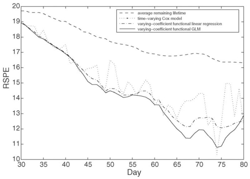
Pointwise average root squared prediction errors (RSPE (9)) for various predictors of remaining lifetime: average remaining lifetime (dashed), time-varying Cox model (dotted), varying-coefficient functional linear model (6) (dash–dot), and varying-coefficient functional generalized linear model (4) (solid), predicting individual remaining lifetime from calling behavior trajectories observed until age t, 30 d ≤ t ≤ 80 d.

$$V(t)=\frac{var(T_i-t)-{\text{RSPE}}^2(t)}{var(T_i-t)}.$$ (10)

This measures the fraction of variance of the observed age-at-death for those subjects at risk at age t is explained by the model.

Inference for these estimates can be obtained via bootstrapping (Manly, 1997). To obtain one bootstrap sample, one resamples n times with replacement from the data of all subjects, sampling one subject at a time. For each such bootstrap sample, one then computes an estimated coefficient ${\beta }_{jt}^{\ast }$ at each time point t. Bootstrap confidence intervals are then obtained from the empirical distribution of these estimated coefficients.

Figs. 1 and 2 describe the time-evolution of the components of the trajectories of calling behavior. We find that the mean and the first eigenfunction evolution are quite smooth, essentially appending new parts smoothly to the previous functions as their domain increases with increasing t, while not dramatically altering function shape on previously included domains. The first eigenfunction has an increasing trend, where the phase of increase shifts with time and is most expressed in an interval of [t − 15, t], where t is current age. The second eigenfunction delineates a broad rising peak and subsequent rapid decline, also centering these features on an interval just before current age. This means that the predictive features of the calling trajectory are concentrated near current age and that calling behavior further in the past of an individual is of much less relevance as compared to recent calling behavior.

Fig. 1.

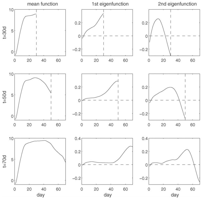
Time-evolution of mean functions (left column, μ̂(·, 30), μ̂(·, 50) and μ̂(·, 70), and of first (middle column, ρ̂_1,30(·), ρ̂_{1, 50}(·) and ρ̂_{1, 70}(·)) and second (right column, ρ̂_{2, 30}(·), ρ̂_{2, 50}(·) and ρ̂_{2, 70}(·)) eigenfunctions for current age t = 30 days (first row), 50 days (second row) and 70 days (third row) days, for male medfly calling data.

Fig. 2.

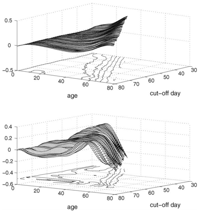
First eigenfunction evolution over time (upper panel, r^_1t(·)) and second eigenfunction evolution (lower panel, r^_2t(·)) for daily calling data (simultaneous display of surface and contour plots). The diagonal from the frontal point (80,80) straight towards the point (0,0) (not shown) indicates current age.

3. Results

3.1. Modes of variation of calling behavior

As about 87.7% of the variation is explained by the first two eigenfunctions (which correspond to the modes of variation for functional data and was obtained by taking the percentage of sum of the first 2 estimated eigenvalues over sum of a reasonable large number of estimated eigenvalues) at t = 50 d, we included M = 2 components. The bandwidths for smoothing mean function and variance-covariance surface were chosen as 3 d and [10 d, 10 d]. The time-evolution of the mean calling function and of the first two eigenfunctions are displayed in Fig. 1 for t = 30, 50, 70 days, respectively.

The continuous eigenfunction evolution alternatively is characteized by a two-dimensional surface on a triangular support, as shown in Fig. 2 for the first two eigenfunctions. The first eigenfunction evolution is seen to be remarkably smooth on this continuous time scale, while the evolution of the second eigenfunction exhibits a small amount of flattening for increasing domains. The parallelity of the peaks with the diagonal line corresponding to current time is quite obvious, confirming that early calling behavior at younger ages does not play an important role in determining remaining longevity.

3.2. Mean remaining lifetime

The estimated functional varying-coefficients β̂_jt for the linear model (6) and also the pointwise bootstrap confidence intervals for the true coefficients are illustrated in Fig. 3. The coefficients (solid line) are seen to vary smoothly in t. Coefficients β̂_0t (solid line in upper panel) provide an estimate of the overall mean remaining life function r₀(t) in Eq. (6) and taper off accordingly with increasing t. Estimates β̂_1t (solid line in the middle panel) exhibit some fluctuation around a small positive value; the bootstrap confidence bands provide evidence that the underlying values are significantly positive most of the time.

Fig. 3.

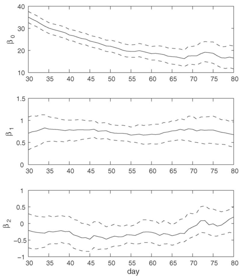
The 95% point-wise bootstrap confidence intervals based on B = 1000 bootstrap samples for the varying coefficients β_0t (top panel), β_1t (middle panel) and β_2t (bottom panel) of the varying-coefficient functional linear model (6), for daily calling data. The solid lines are the coefficient estimates β̂_0t, β̂_1t and β̂_2t.

This translates into the finding that cost in terms of decreased remaining lifetime tends to be the higher, the smaller the corresponding estimate of the first functional principal component score ε̂_i1t is. Larger coefficients and therefore stronger alignment of an individual with the first eigenfunction shown in Fig. 1 corresponds to enhanced longevity.

We conclude that recent high and increasing calling activity is associated with extended life span, and this is true across all ages. The effect of the second functional principal component was not significant.

The trajectories at t = 50 d for three flies with varying levels of the first functional principal component scores are plotted in Fig. 4. The respective predictors (estimated functional principal component scores) ε̂_1t are −31.75 (upper panel), 4.16 (middle panel) and 17.22 (lower panel). The fly in the top panel has a trajectory with a rapidly rising peak around day 15 and subsequent slow decline, with overall lower calling levels than the mean curve; its remaining lifetime (beyond the current age of 50 days) was 6 days. The fly in the middle panel also has a peak around day 15 d but then the trajectory tapers off with increasing age as it approaches the current age of t = 50 days. The remaining lifetime of this fly was 35 days. Finally, the fly in the bottom panel has a broader rising peak and only slight decline towards the right boundary, with overall higher values than the overall mean would imply. Its remaining lifetime was 87 days. According to our model, the order of the observed values of ε̂_1t predicts the order of the observed lifetimes, as smaller values of the first functional principal component are expected to be associated with reduced remaining longevity and higher risk.

Fig. 4.

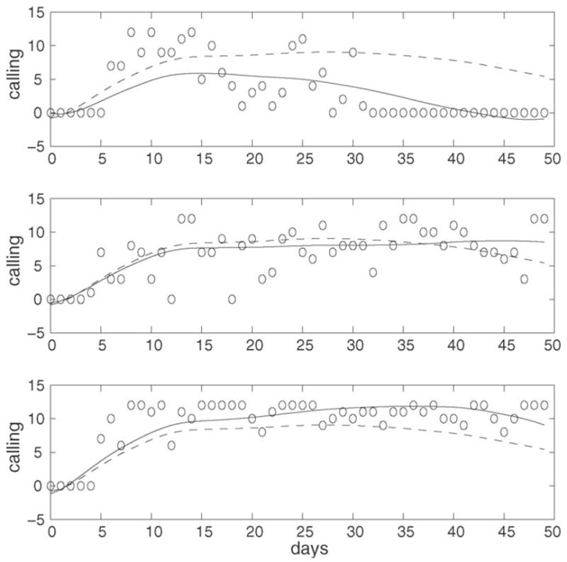
Estimated calling trajectories (solid) for three flies at three different levels for the first principal component score, ε̂_1t = −31. 75 (upper panel), 4.16 (middle panel), 17.22 (lower panel), overlaid with the mean function μ̂(t, s) (dashed) and the original measurements (circles) of calling frequency, for age t = 50 days.

3.3. Conditional distributions

The proposed methodology also allows to estimate the conditional distribution of remaining lifetime from the calling trajectory X̃ for an individual up to age t. As an example, for age t = 40 days, we may select two flies at different levels of the linear predictor η(t), η₁(t) = −8.3893 (age-at-death T₁ = 43 d) for the first fly and η₂(t) = 8.0760 (age-at-death T₂ = 57 d) for the second fly. Their calling trajectories up to t = 40 d are shown in the left panels of Fig. 5, along with the observed data. The corresponding conditional density function estimates of remaining lifetime, based on these calling histories, are shown in the right panels.

Fig. 5.

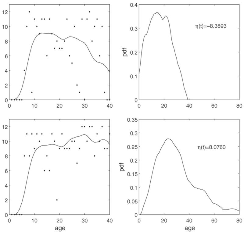
Calling trajectories and original observations for two male flies are shown up to age t = 40 d for a fly with linear predictor η̂₁(40) = −8.3893 and remaining lifetime T₁ = 43 days, and a fly with linear predictor η̂₂(40) = 8.0760 and remaining lifetime T₂ = 57 days (left panels). The corresponding predicted conditional density estimates for remaining lifetime distribution for these individual flies are shown in the right panels.

The predictions associated with the shapes of the calling trajectories in the left panels of Fig. 5 are typical. While for the fly in the upper panels calling frequency is decreasing after 20 days and the decrease is quite rapid, calling frequency for the second fly in the lower panels is sustained into current age and even is slightly increasing after age 15 days. These different calling behavior patterns lead to corresponding differences in predicted conditional densities, with more expected longer remaining lifetimes and higher longevity (correctly) predicted for the second fly. Remaining longevity thus is found to be closely related to the shape of the calling trajectory.

The time-evolution of the estimated evaluation functions β̂(s, t) is displayed in Fig. 6, where these functions are seen to depend smoothly on age t. A clear pattern emerges: Increased calling activity near the end of a current observed period leads to increased values of the single index predictor η, and is indicative of increased remaining lifespan, while early calling activity (occurring more than 15 d prior to the current day at which remaining lifetime is to be predicted) plays not much of a role and is largely irrelevant for future longevity.

Fig. 6.

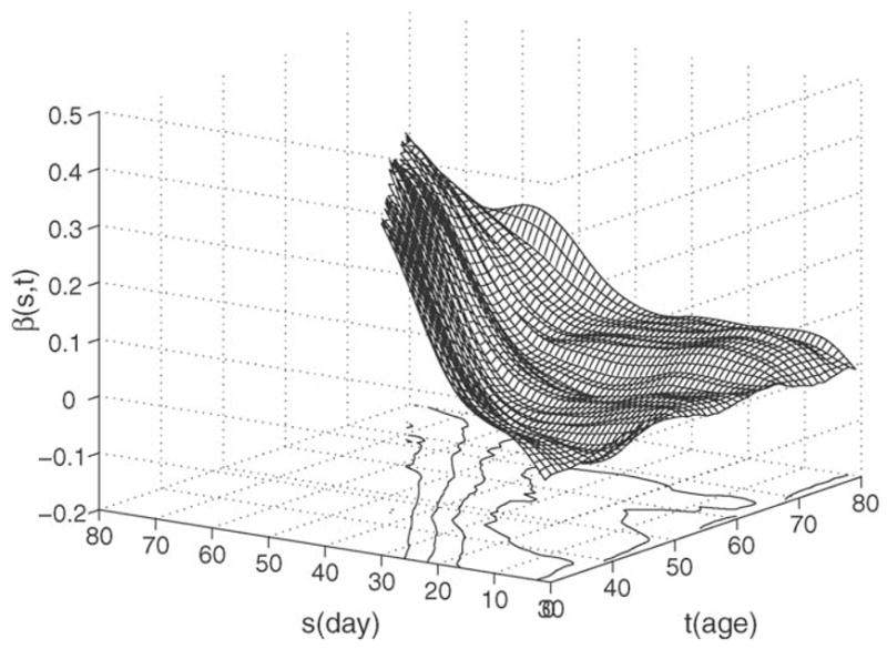
Evolution of the evaluation functions $\beta (s,t)={\sum }_{j=1}^M{\beta }_{jt}{\rho }_{jt}(s)$, 0 ≤ s ≤ t, over time in the semiparametric regression model (4) with simultaneous display of surface and contour plots.

The upper panel of Fig. 7 visualizes the relation between the calling histories and the linear predictor η(t). The relation is seen to be governed primarily by the behavior near the end of each current period (here t = 50 d was chosen), higher levels of calling behavior being associated with larger values of η, consistent with the earlier findings from the evaluation function β̂(s, t). As the lower panel of Fig. 7 demonstrates, larger values of η̂ are associated with long-tailed predicted densities for remaining lifetime and enhanced remaining longevity, while small values of η̂ are associated with peaked densities with short tails and shortened remaining longevity. The main message from this analysis is that high and increasing calling activity close to current age is associated with increased remaining longevity for individual flies. The relationship of this patterns is surprisingly clear-cut and demonstrates the power of this methodology in applications.

Fig. 7.

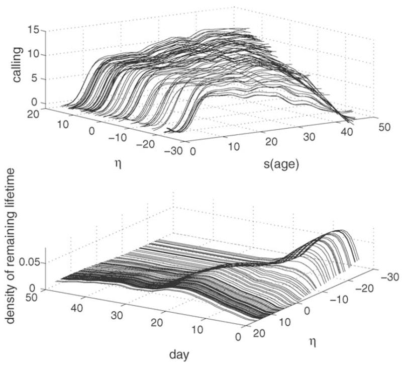
Observed trajectories of calling behavior (upper panel) from birth to current age t = 50 days and estimated densities of remaining lifetime after age 50 d (lower panel), both in dependency on the value of the estimated single index function η̂(t) (5). Curves at the same values of η̂ correspond to each other.

3.4. Methods comparison and variance explained by calling trajectories

The performance in terms of root squared prediction error RSPE (9) of average remaining lifetime was compared for various methods at several ages, based on the observed calling data. The comparison included the varying-coefficient functional linear model (6), the varying-coefficient functional generalized linear model (4) and the time-varying Cox model for remaining lifetime estimation and used the one-leave-out prediction error as criterion for the comparisons (see also Müller and Zhang, 2005). The results are presented in Fig. 8. We find that average remaining lifetime as a predictor, not surprisingly, has the largest RSPE, and the varying-coefficient functional generalized linear model the smallest, especially at older ages.

We also compared the relative gain in terms of variance of remaining lifetime explained through the function V(t) (9) for various methods. This comparison is illustrated in Fig. 9. Average remaining lifetime as a predictor achieves zero relative gain as it establishes the baseline variance of remaining lifetime that needs to be explained by the observed calling trajectories. We find that QLUE has the overall largest relative gain and therefore is the method which explains the largest fraction of the variance of remaining lifetime.

Fig. 9.

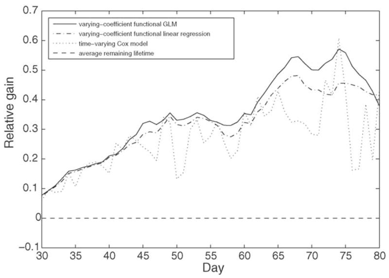
Relative gain function V(t) (9) for various predictors of remaining lifetime: average remaining lifetime (dashed), time-varying Cox model (dotted), varying-coefficient functional linear model (6) (dash–dot), and varying-coefficient functional generalized linear model (4) (solid). The function depicts the fraction of variance explained by the trajectory of male calling observed until age t.

The variance explained increases with increasing age, which means that at older ages the calling activity is increasingly associated with the length of remaining life. This means that the level of calling activity is increasingly an indicator of remaining life as a fly ages. It is noteworthy that the QLUE method for predicting individual remaining lifetime explains more than 55% of the variance of remaining lifetime at age t = 75 d. This is a far larger fraction of the variance than normally are expected to be explained by covariates in biodemographic studies.

4. Discussion

It is biologically reasonable that intensive sexual signalling can only be possessed by strong, fit individuals, who also have a good chance to postpone death (Barnard, 1983). We find here that the level of sexual calling behavior in a 15 day interval prior to current age is a good predictor of remaining lifetime and residual life span. We note that these results complement the event history graphs (Carey et al., 1998) that were constructed for calling behavior of male medflies in Fig. 3 of Carey et al. (2006). When comparing remaining lifetime for individual flies at a fixed age, we find that those flies with higher calling behavior at the fixed age generally have higher remaining lifetime. Especially if the level of current calling is low then remaining lifetime is also low. The current analysis refines this graphical association and provides a formal model for evaluating such relationships.

Since the first eigenfunction features a sharp increase just prior to current time, there seems to be no cost associated with past calling behavior and as far as calling behavior is concerned, remaining longevity is exclusively determined by very recent levels of calling. Higher frequency of recent calling unambiguously signals lower risk. The situation is quite different for female medflies (Müller and Zhang, 2005), where one observes a cost associated with an early rapid rise to high egg-laying levels, which is form of cost of reproduction that persists into older ages.

In the light of our findings, one may conclude that sexual calling activity incurs no cost on male medflies and serves as an indicator of their current status in terms of health and robustness as measured in their propensity for survival. The proposed methodology can also be used to predict other future characteristics of an individual fly from the life history observed to time t, rather than remaining lifetime at age t. For example, for female flies one could predict the remaining number of eggs laid between t and age-at-death T, based on the observations of egg-laying or other behaviors until time t, which then may reveal dynamics of egg-laying, reproduction and their interplay with longevity, extending previous approaches of Müller et al. (2001).

We conclude that the methodology of functional data analysis, functional principal components and time-varying functional regression that has been demonstrated here is of broad interest for event history analysis and the analysis of biodemographic data. Regarding calling behavior of male medflies it leads to valuable insights into the determinants of remaining survival based on the shape of predictor trajectories.

References

- Barnard CJ. Animal Behaviour: Ecology and Evolution. Wiley; New York: 1983. [Google Scholar]
- Carey JR, Liedo P, Müller H-G, Wang J-L, Vaupel JW. A simple graphical technique for displaying individual fertility data and cohort survival: case study of 1000 Mediterranean fruit fly females. Funct Ecol. 1998;12:359–363. [Google Scholar]
- Carey JR, Papadopoulos NT, Kouloussis NA, Katsoyannos BI, Müller HG, Wang JL, Tseng YK. Age-specific and lifetime behavior patterns in Drosophila melanogaster and the Mediterranean fruit fly, Ceratitis capitata. Exp Gerontol. 2006;41:93–97. doi: 10.1016/j.exger.2005.09.014. [DOI] [PMC free article] [PubMed] [Google Scholar]
- Castro PE, Lawton WH, Sylvestre EA. Principal modes of variation for processes with continuous sample curves. Technometrics. 1986;28:329–337. [Google Scholar]
- Chiou JM, Müller HG. Quasi-likelihood regression with unknown link and variance functions. J Am Stat Assoc. 1998;93:1376–1387. [Google Scholar]
- Chiou JM, Müller HG. Nonparametric quasi-likelihood. Ann Stat. 1999;27:36–64. [Google Scholar]
- Cox DR. Regression models and life tables (with discussion) J R Stat Soc Ser B. 1972;34:187–200. [Google Scholar]
- Manly BFJ. Randomization, Bootstrap and Monte Carlo Methods in Biology. Chapman and Hall; London: 1997. [Google Scholar]
- Müller HG. Functional modelling and classification of longitudinal data. Scand J Stat. 2005;32:223–240. [Google Scholar]
- Müller HG, Carey JR, Wu D, Liedo P, Vaupel JW. Reproductive potential predicts longevity of female Mediterranean fruit flies. Proc R Soc B. 2001;268:445–450. doi: 10.1098/rspb.2000.1370. [DOI] [PMC free article] [PubMed] [Google Scholar]
- Müller HG, Zhang Y. Time-varying functional regression for predicting remaining lifetime distributions from longitudinal trajectories. Biometrics. 2005;61:1064–1075. doi: 10.1111/j.1541-0420.2005.00378.x. [DOI] [PMC free article] [PubMed] [Google Scholar]
- Papadopoulos NT, Katsoyannos BI, Kouloussis NA, Carey JR, Müller H-G, Zhang Y. High sexual signalling rates of young individuals predict extended life span in male Mediterranean fruit flies. Oecologia. 2004;138:127–134. doi: 10.1007/s00442-003-1392-3. [DOI] [PMC free article] [PubMed] [Google Scholar]
- Ramsay J, Silverman B. Applied Functional Data Analysis. Springer; New York: 2002. [Google Scholar]
- Ramsay J, Silverman B. Functional Data Analysis. Springer; New York: 2005. [Google Scholar]
- Rao CR. Some statistical methods for the comparison of growth curves. Biometrics. 1958;14:1–17. [Google Scholar]
- Rice J, Silverman B. Estimating the mean and covariance structure nonparametrically when the data are curves. J R Stat Soc Ser B. 1991;53:233–243. [Google Scholar]
- Yashin AI, Manton KG. Effects of unobserved and partially observed covariate processes on system failure: a review of models and estimation strategies. Stat Sci. 1997;12:20–34. [Google Scholar]