Information-Theoretic Analysis of Brain White Matter Fiber Orientation Distribution Functions

Abstract

We propose a new information-theoretic metric, the symmetric Kullback-Leibler divergence (sKL-divergence), to measure the difference between two water diffusivity profiles in high angular resolution diffusion imaging (HARDI). Water diffusivity profiles are modeled as probability density functions on the unit sphere, and the sKL-divergence is computed from a spherical harmonic series, which greatly reduces computational complexity. Adjustment of the orientation of diffusivity functions is essential when the image is being warped, so we propose a fast algorithm to determine the principal direction of diffusivity functions using principal component analysis (PCA). We compare sKL-divergence with other inner-product based cost functions using synthetic samples and real HARDI data, and show that the sKL-divergence is highly sensitive in detecting small differences between two diffusivity profiles and therefore shows promise for applications in the nonlinear registration and multi-subject statistical analysis of HARDI data.

1 Introduction

High angular resolution diffusion imaging (HARDI) is a variant of conventional MRI that uses multiple radially-distributed gradients to encode directional profiles and orientations of water diffusion [1]. In conventional diffusion tensor imaging (DTI), the 3D diffusion profile of water molecules at each point in the brain is considered to have an ellipsoidal profile, which can be modeled using a second-rank tensor. Theoretically, 7 diffusion-encoding gradients are sufficient for fitting a tensor. By contrast, HARDI applies many more diffusion-encoding gradients to measure diffusivity at high angular resolution, revealing the detailed orientation profile for water diffusion within each voxel. Diffusivity profiles can be resolved more clearly in brain regions where fiber tracts cross, providing more accurate information for fiber-tracking (tractography), disease detection, and analysis of anatomical connectivity.

Several successful algorithms exist for linear and nonlinear registration of DTI [2–4]. Registration of HARDI data has not been widely studied, perhaps because HARDI yields high-dimensional datasets, often with 30–100 observations per voxel (corresponding to the number of gradient directions), compared with 6 independent parameters per voxel in DTI. Modeling and comparing diffusivity profiles is therefore computationally expensive, but vital for guiding alignment (registration) of HARDI data across subjects or time, prior to multisubject statistical analysis.

Several cost functions have been proposed for DTI registration, such as Euclidean or log-Euclidean distance between two diffusion profiles, or the multichannel sum of squared differences (SSD) [5]. Here we evaluate a new information-theoretic metric, the symmetric Kullback-Leibler divergence (sKL-divergence), for measuring differences between diffusivity profiles in HARDI. Information theory is relevant for estimating diffusivity profiles and also for measuring anisotropy (e.g., the cumulative residual entropy method [6, 7]). Vemuri [8] successfully used the sKL-divergence to measure the distance between two Gaussian tensors, for DTI segmentation. Here we compute sKL-divergence from spherical harmonic expansions of the orientation-dependent diffusion functions (ODFs). Spherical harmonic series are widely used in HARDI visualization and regularization [9, 10]; they can help in efficiently computing the diffusion displacement probabilities [11], and visualizing the ODF at each voxel [12]. We show that sKL-divergence is more robust than standard inner product measures for detecting small rotational deviations between HARDI data, at various diffusion weights and noise levels, making it an attractive measure for HARDI registration.

2 Methods

2.1 Kullback-Leibler Divergence of Two Diffusivity Functions

In HARDI, the signal attenuation in a specific direction, g, is given by the Stejskal-Tanner equation [13]:

$$S(g)=S_{0}exp(-bD(g)).$$ (1)

where b is the diffusion weighting factor, D is the scalar diffusivity (apparent diffusion coefficient) and g is the diffusion-encoded gradient direction, with g = g(θ, φ) = [sin θ cos φ sin θ sin φ cos θ]^T; θ and φ are the polar and azimuthal angles. Inspired by [14], we model the diffusivity function as a probability density function (pdf), by normalizing its integral over the spherical angle Ω to 1:

$$\begin{array}{l}p(\theta ,\phi )=D(\theta ,\phi )/\mathit{gtr}(D),\\ \mathit{gtr}(D)=\underset{\mathrm{\Omega }}{\int }D(\theta ,\phi )d\mathrm{\Omega },\end{array}$$ (2)

where gtr is the generalized trace of D [14]. For two diffusivity functions D_p and D_q, we define the symmetric KL-divergence based on the corresponding pdfs p(θ, φ) and q(θ, φ):

$$\begin{array}{l}\mathit{sKL}(p,q)=\frac{1}{2}\left\{\underset{\mathrm{\Omega }}{\int }plog(\frac{p}{q})d\mathrm{\Omega }+\underset{\mathrm{\Omega }}{\int }qlog(\frac{q}{p})d\mathrm{\Omega }\right\}\\ =\frac{1}{2}\left\{\begin{array}{l}\underset{\mathrm{\Omega }}{\int }plog(p)d\mathrm{\Omega }-\underset{\mathrm{\Omega }}{\int }plog(q)d\mathrm{\Omega }+\underset{\mathrm{\Omega }}{\int }qlog(q)d\mathrm{\Omega }\hfill \\ -\underset{\mathrm{\Omega }}{\int }qlog(p)d\mathrm{\Omega }\hfill \end{array}\right\}.\end{array}$$ (3)

Applying Eq (2) to the integrals in Eq (3), for example,

$$\begin{array}{l}\underset{\mathrm{\Omega }}{\int }plog(q)d\mathrm{\Omega }=\underset{\mathrm{\Omega }}{\int }\frac{D_p}{\mathit{gtr}(D_p)}[log(D_q)-log(\mathit{gtr}(D_q))]d\mathrm{\Omega }\\ =\left[\frac{1}{\mathit{gtr}(D_p)}\underset{\mathrm{\Omega }}{\int }{D}_{p}log(D_q)d\mathrm{\Omega }\right]-log(\mathit{gtr}(D_q)),\end{array}$$ (4)

we then have

$$\mathit{sKL}(p,q)=\frac{1}{2}\left\{\begin{array}{l}\frac{1}{\mathit{gtr}(D_p)}\left[\underset{\mathrm{\Omega }}{\int }{D}_{p}log(D_p)d\mathrm{\Omega }-\underset{\mathrm{\Omega }}{\int }{D}_{p}log(D_q)d\mathrm{\Omega }\right]\hfill \\ +\frac{1}{\mathit{gtr}(D_q)}\left[\underset{\mathrm{\Omega }}{\int }{D}_{q}log(D_q)d\mathrm{\Omega }-\underset{\mathrm{\Omega }}{\int }{D}_{q}log(D_p)d\mathrm{\Omega }\right]\hfill \end{array}\right\}.$$ (5)

Direct estimation of sKL in Eq (5) is computationally expensive, but is faster if we expand the diffusivity functions D(θ, φ) as a spherical harmonic (SH) series [9, 10]:

$$\begin{array}{l}D(\theta ,\phi )=\sum _{l=0}^{\infty }\sum _{m=-l}^l{c}_l^m{Y}_l^m(\theta ,\phi ),\\ Y_l^m(\theta ,\phi )=\sqrt{\frac{(2l+1)}{4\pi }\frac{(l-m)!}{(l+m)!}}{P}_l^m(cos\theta )e^{im\theta };\end{array}$$ (6)

here $P_l^m(cos\theta )$ are the associated Legendre polynomials. D(θ, φ) is real and radially symmetric, so it is sufficient to adopt a real basis function set Y_lm while retaining the orthonormality of $Y_l^m$ [10]:

$$\begin{array}{l}D(\theta ,\phi )=\sum _{l=0,\mathit{even}}^{\infty }\sum _{m=-1}^l{c}_{lm}{Y}_{lm}(\theta ,\phi ),\\ Y_l^m=\{\begin{array}{c}\frac{\sqrt{2}}{2}({(-1)}^m{Y}_l^m+Y_l^{-m}),\text{ if }-l\le m<0\\ Y_l^0,\text{ if }m=0\\ \frac{\sqrt{2i}}{2}({(-1)}^{m+1}{Y}_l^m+Y_l^{-m}),\text{ if }0<m\le l\end{array}l=0,2,4,\dots \end{array}$$ (7)

As the Y_lm are orthonormal, the inner product of the real functions D₁ and D₂ can be expressed in terms of their SH coefficients $(c_{lm}^{D_1}\text{ and }{c}_{lm}^{D_2})$:

$$\underset{\mathrm{\Omega }}{\int }{D}_1(\theta ,\phi )D_2(\theta ,\phi )d\mathrm{\Omega }=\sum _{l=0,\mathit{even}}^{\infty }\sum _{m=-l}^l{c}_{lm}^{D_1}{c}_{lm}^{D_2}.$$ (8)

Moreover, it can be shown that (see Appendix for derivations):

$$\underset{\mathrm{\Omega }}{\int }D(\theta ,\phi )d\mathrm{\Omega }=2\sqrt{\pi }{c}_{00}.$$ (9)

Therefore, sKL in Eq (5) can be expanded in terms of the SH series, as follows:

$$\mathit{sKL}(p,q)=\frac{1}{2}\left\{\begin{array}{l}\frac{1}{c_{00}^p}\sum _{l=0,\mathit{even}}^{\infty }\sum _{m=-l}^l[c_{lm}^p{d}_{lm}^p-c_{lm}^p{d}_{lm}^q]\hfill \\ +\frac{1}{c_{00}^q}\sum _{l=0,\mathit{even}}^{\infty }\sum _{m=-l}^l[c_{lm}^q{d}_{lm}^q-c_{lm}^q{d}_{lm}^p]\hfill \end{array}\right\},$$ (10)

where $D_j={\displaystyle \sum _{l=0,\mathit{even}}^{\infty }}{\displaystyle \sum _{m=-l}^l}{c}_{lm}^j{Y}_{lm},log(D_j)={\displaystyle \sum _{l=0,\mathit{even}}^{\infty }}{\displaystyle \sum _{m=-l}^l}{d}_{lm}^j{Y}_{lm},\text{ and }j\in \{p,q\}$.

For numerical implementation, we use a truncated SH series with l ≤ l_m, where l_m is a positive even integer; the total length of the SH series is n_b = (l_m+1)(l_m+2)/2. We follow the least-squares method [9, 10] to solve Eq (7), yielding the SH coefficients:

$$C={(B^{T}B)}^{-1}{B}^{T}D.$$ (11)

Here C=[c₀ c₁ · · c_nb−1]^T, and D = [D(θ_0, φ₀) D(θ_1, φ₁)· · D(θ_ns, φ_ns)]^T which represents the diffusivity function measured in n_s gradient directions, and B is the matrix of basis functions, with elements B_ij = Y_j (θ _i, φ _i). Here we map (c_lm, Y_lm) in Eq (7) to (c_j, Y_j), using the relationship j = [(l²+l)/2] + m. Usually n_b ≪ n_s, so it is more cost-effective to compute sKL using the SH method (Eq (10)) rather than using Eq (5) directly.

2.2 Reorientation of Diffusivity Functions

Similar to diffusion tensors in DTI, the diffusivity functions in HARDI are oriented and their directions must be adjusted when the HARDI data are linearly or nonlinearly transformed. We adopt the “Preservation of Principal Directions (PPD)” method [15], which preserves the shape of the diffusivity function along the local principal fiber orientation. With DTI, given the local Jacobian matrix J of the image transformation, the PPD procedure yields a rotation matrix that rotates the first eigenvector e₁ onto Je₁/|Je₁| and the second eigenvector e₂ onto the plane spanned by Je₁/|Je₁| and Je₂/|Je₂| In HARDI, however, a single diffusivity function may have multiple local maxima that are computationally expensive to determine [16], and thus not practical to perform at every iteration during image warping. Here we propose a fast algorithm to determine the principal direction of the diffusivity function, based on the principal component analysis (PCA) of its shape [17]. At each direction sampled by the diffusion gradient g(θ_i, φ_i), 0 ≤ i < n_s, we define a point with distance to the origin d_i = D(θ_i, φ_i) g(θ_i, φ_i) = (d_i0, d_i1, d_i2), where the last term is the Cartesian coordinates of d_i. The mean and the covariance matrices, μ and Σ, of the point set {d_i} are given by

$${\mu }_j=\frac{1}{n_s}\sum _{i=0}^{n_s-1}{d}_{ij};{\sum }_{ij}=\frac{1}{n_s}\sum _{k=0}^{n_s-1}(d_{ki}-{\mu }_i)(d_{kj}-{\mu }_j),0\le i,j<3.$$ (12)

The principal direction of the diffusivity function is determined by the first eigenvector of Σ. The rotation matrix R, which adjusts the direction of the diffusivity function, is then obtained using the PPD procedure, and the new gradient directions $g({\theta }_i^{\prime },{\phi }_i^{\prime })=R\cdot g({\theta }_i,{\phi }_i)$.

However, it is advantageous to have values of the reoriented diffusivity function in the original directions (θ_i, φ_i), rather than the new ones $({\theta }_i^{\prime },{\phi }_i^{\prime })$, because (1) we do not need to keep track of new reoriented gradient directions at each iteration of image warping, and (2) sKL (or other cost functions) can be compared on diffusivity functions sampled at identical gradient directions for the target image (which is fixed) and the source (which is moving and in which the diffusivity functions are being reoriented). Because the gradient directions are only discretely sampled, the reoriented diffusivity functions are constructed by “pushing” the values sampled at the original directions to the new directions, so the values of the reoriented function at the original directions are not known. These new values can be computed from the SH series, as the basis functions Y_lm are continuous and defined at all spherical angles. If $(\mathrm{\Delta }{\theta }_i,\mathrm{\Delta }{\phi }_i)=({\theta }_i^{\prime }-{\theta }_i,{\phi }_i^{\prime }-{\phi }_i)$, then the values of the reoriented diffusivity functions D′ in the original directions (θ_i, φ_i) are given by

$$D^{\prime }({\theta }_i,{\phi }_i)=D({\theta }_i-\mathrm{\Delta }{\theta }_i,{\phi }_i-\mathrm{\Delta }{\phi }_i)=\sum _{l=0\mathit{even}}^{\infty }\sum _{m=-l}^l{c}_{lm}{Y}_{lm}({\theta }_i-\mathrm{\Delta }{\theta }_i,{\phi }_i-\mathrm{\Delta }{\phi }_i),$$ (13)

where c_lm are the SH coefficients of the original diffusivity function D (see Eq (7)).

2.3 Interpolation of Diffusivity Functions

Diffusivity functions must be interpolated when the HARDI data is warped and the new voxel locations are not on lattice points. It is natural to interpolate diffusivity functions separately for each gradient direction (i.e., multichannel interpolation). We therefore performed linear interpolation of D(θ _i, φ _i), log(D(θ _i, φ _i)), and of the MR signals S(θ _i, φ _i) in synthetic samples and compared the swelling effect (i.e., loss of anisotropy) of these three interpolation schemes.

3 Experiments and Results

Synthetic examples

We constructed a two-fiber diffusivity function using two orthogonal Gaussian tensors, T₀ and T₁, with typical eigenvalues for white-matter (WM) fibers [9, 10]. We set T₀ = diag(200, 200, 1700) × 10⁻⁶ (mm²/s); T₁ was obtained by rotating T₀ 90 degrees around the y-axis. We also generated an isotropic gray-matter (GM) diffusivity function by setting T_iso = diag(700, 700, 700) × 10⁻⁶ (mm²/s). Then the diffusivity function D is given by

$$D=-\frac{1}{b}\sum _{i=0}^{n-1}{p}_{i}exp(-b{g}^T{T}_{i}g),$$ (14)

where n is the number of fibers. p₀ = p₁ = 0.5 for two-fiber structures and p₀ = 1 for the isotropic diffusivity function. The gradient direction vector g consisted of 162 sampled points determined using an electrostatic approach [18]. Different b values (500, 1500, 3000) s/mm² were tested. The order of the SH series (l_m) was set to 8.

HARDI data

The HARDI data was acquired from a healthy 22-year-old man imaged as part of a research study of twins on a 4T Bruker Medspec MRI scanner using an optimized diffusion tensor sequence [18]. Imaging parameters were: 21 axial slices (5 mm thick), FOV = 24 cm, TR/TE 6090/104.5 ms, 0.5 mm gap, with a 128×100 acquisition matrix and 30 images acquired at each location: 3 low (b = 0) and 27 high diffusion-weighted images in which the encoding gradient vectors were uniformly radially distributed in space (b = 1100 s/mm²) using the electrostatic approach in [18]. The reconstruction matrix was 128×128, yielding a 1.875×1.875 mm² in-plane resolution. The total scan time was 3.09 minutes. We set l_m = 4 for the spherical harmonic analysis.

Fig. 1 shows that the principal directions determined from HARDI by the PCA method are compatible with those computed by DTI and persistent angle structures (PAS) fitting using the software Camino developed at University College, London [19], in major WM fiber structures. Fig. 2 compares the fiber directions when the HARDI data was rotated by 60 degrees around the inferior-superior axis passing through its center of mass, with and without reorientation of the diffusivity functions. As observed in [15, 20], our results show that the orientation of the diffusivity functions must be adjusted when the image is transformed, to maintain the spatial coherence of the principal fiber directions. To do this, we used the PPD procedure, which is more accurate than other methods (e.g., Finite Strain [3, 15]) as it takes the original fiber directions into account. PCA determines one eigendirection, so it is appropriate for diffusivity functions with a single global maximum, or with a dominant local maximum relative to other small local maxima. In diffusivity functions with multiple local maxima, such as in regions where fibers cross (e.g. the synthetic samples in Fig. 3), the principal direction estimated by PCA becomes arbitrary, and the simple PPD procedure may not be applicable in these regions.

Fig. 1.

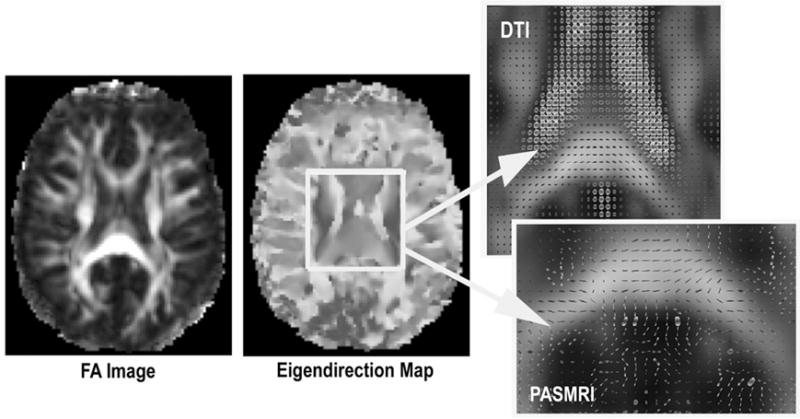
The eigendirection map for the HARDI data, determined using the PCA method. Fibers with right-left orientation are shown in red, anterior-posterior in green, and inferior-superior in blue. The eigendirections correctly depict the orientations of major WM fiber structures, and are compatible with the tensor glyphs and PAS computed using the visualization software “Camino” [19]. FA: fractional anisotropy.

Fig. 2.

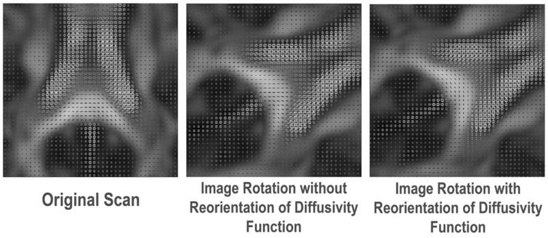
The orientation-dependent diffusivity functions in the splenium of the corpus callosum are no longer consistent with the known directions of the underlying WM fibers when the image voxels are simply resampled to new locations by rotation but without reorientation of diffusivity functions. The PPD procedure corrects this, and the diffusivity functions remain aligned with the WM fibers that they represent.

Fig. 3.

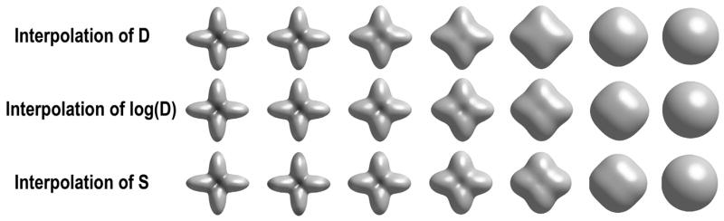
Comparison of diffusivity functions obtained by linear interpolation of D, log(D) and S. Interpolation using the MR signal S best preserves the anisotropy of the diffusivity function.

Fig. 3 shows diffusivity functions at intermediate positions x = 0.1, 0.3, .. 0.9, obtained by linear interpolation of the diffusivity function D, log(D), and MR signals S in each gradient direction, when the two-fiber synthetic function was placed at x = 0, and the isotropic one at x = 1.

Direct interpolation of the MR signals results in the least swelling, or loss of anisotropy, in the diffusivity function. Euclidean interpolation may also be more appropriate for the MR signals, which are physical entities. Linear interpolation using log(D) performs better than D (as least in terms of degrading the signal geometry). Computing log(D) may therefore be an acceptable alternative to computing S. Log(D) can be computed in the spherical harmonic domain (see Eq (10)), which is more economical in terms of memory than performing interpolation on S - this may be beneficial for HARDI registration.

We compared the symmetric KL-divergence (sKL) with other two cost functions, the inner product of diffusivity functions in Eq (8) with and without the linear (l = 0) term [3, 21], on synthetic examples that were noise-free, or with Rician noise added to MR signals S such that the signal-to-noise ratio (SNR) was 35 or 10 [22]. The inner product without the l = 0 term is designed to compare only the anisotropic part of the diffusivity functions [3]. Two identical two-fiber synthetic diffusivity functions served as the source and the target objects, with the source object rotating from 0 (complete overlap) to 90 degrees. The three metrics were normalized for comparisons (as detailed in Fig. 4). Fig. 4 shows that at different noise levels, the sKL cost function detects angular discrepancies in diffusivity functions more sensitively than the inner product with/without the l = 0 term, in low b-settings. sKL is also still comparable in performance with the inner product without l = 0 term, at a high b-value. The performance of sKL is therefore stable under various diffusion weightings, and it is applicable in ordinary MRI/DTI acquisition settings, though a high b-value can detect higher-order angular structures in WM fibers, at the cost of a decreased SNR [1].

Fig. 4.

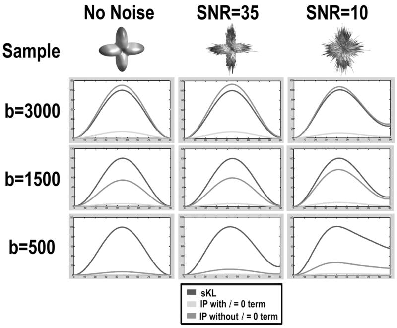
Two identical synthetic diffusivity samples (no noise or with Rician noise added) were initially overlapped and rotated by ϕ = 0 to 90°. We compared the differences between the rotated and non-rotated samples with the symmetric KL-divergence (sKL) and inner product (IP) with/without l = 0 term. In noise-free samples, ϕ = 45° gives the maximum sKL and minimum IP values. To facilitate comparisons, sKL and IP values have been normalized such that the normalized sKL(ϕ) = 100 × sKL(ϕ)/sKL(ϕ = 45°), and normalized IP(ϕ) = 100 × [1 − IP(ϕ)/IP(ϕ = 0°)].

We further compared the three cost functions, which were summed over all voxels, in the 3D HARDI data. Two identical HARDI data was initially overlapped (rotation angle = 0 degree), and then one image was rotated (with diffusivity functions reoriented) up to ±20 degrees, with sKL and inner products (with/without l = 0 term) computed at every two degrees. Fig. 5 shows that sKL has very sharp gradient near the optimal solution, and is sensitive enough to detect 2-degree deviation of the images. The symmetric KL-divergence is therefore a good candidate cost function for registration of HARDI, which we expect to evaluate in the near future.

Fig. 5.

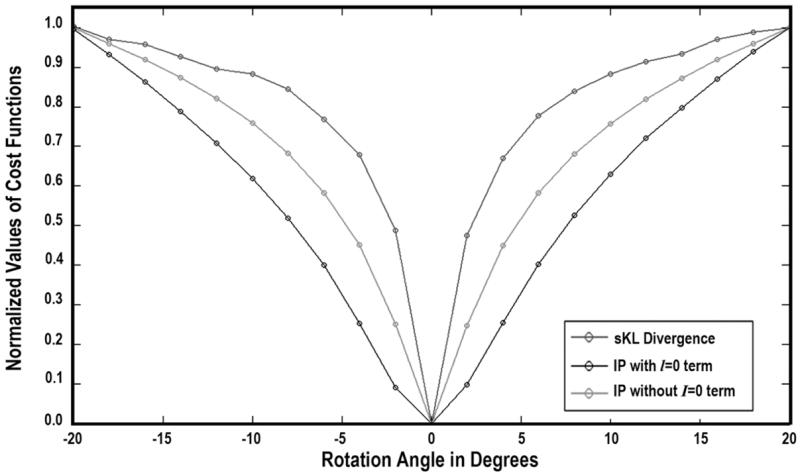
Comparisons of the changes in symmetric KL-divergence (sKL) and inner product (IP) (with/without l = 0 term) at different rotation angles ϕ (from −20° to +20°, in increments of 2°) for two identical HARDI diffusion profiles. sKL and IP values have been normalized, with normalized f(ϕ) = abs[(f(ϕ) − f(ϕ = 0°))/(f(ϕ = 20°) − f(ϕ = 0°))]. The angular profile of sKL is very sharp, and can detect rotational deviations of the image, with a magnitude as small as 2°.

Appendix

$$\begin{array}{l}\underset{\mathrm{\Omega }}{\int }D(\theta ,\phi )d\mathrm{\Omega }=\underset{\theta =0}{\overset{\pi }{\int }}\underset{\phi =0}{\overset{2\pi }{\int }}\sum _{l=0,\mathit{even}}^{\infty }\sum _{m=-l}^l{c}_{lm}{Y}_{lm}(\theta ,\phi )d\phi sin\theta d\theta \\ =\sum _{l=0,\mathit{even}}^{\infty }{c}_{l0}\underset{0}{\overset{\pi }{\int }}\underset{0}{\overset{2\pi }{\int }}{Y}_{l0}(\theta ,\phi )d\phi sin\theta d\theta \\ +\sum _{l=0,\mathit{even}}^{\infty }\sum _{m=-l,m\ne 0}^l{c}_{lm}\underset{0}{\overset{\pi }{\int }}\underset{0}{\overset{2\pi }{\int }}{Y}_{lm}(\theta ,\phi )d\phi sin\theta d\theta .\end{array}$$ (A1)

Given that

$$\begin{array}{l}{\int }_0^{\pi }{\int }_0^{2\pi }{Y}_l^m(\theta ,\phi )d\phi sin\theta d\theta =\sqrt{\frac{(2l+1)}{4\pi }\frac{(l-m)!}{(l+m)!}}{\int }_0^{\pi }{P}_l^m(cos\theta )sin\theta d\theta \\ \cdot \left({\int }_0^{2\pi }{e}^{im\phi }d\phi \right)\\ =0,\text{ if }m\ne 0,\end{array}$$ (A2)

since ${\int }_0^{2\pi }{e}^{im\phi }d\phi =0,\text{ if }m\ne 0$, we have

$$\sum _{l=0,\mathit{even}}^{\infty }\sum _{m=-l,m\ne 0}^l{c}_{lm}\underset{0}{\overset{\pi }{\int }}\underset{0}{\overset{2\pi }{\int }}{Y}_{lm}(\theta ,\phi )d\phi sin\theta d\theta =0.$$ (A3)

Here we use the definition of Y_lm in Eq (7), where Y_lm comes from linear combinations of $Y_l^m$. Therefore, Eq (A1) becomes

$$\begin{array}{l}\underset{\mathrm{\Omega }}{\int }D(\theta ,\phi )d\mathrm{\Omega }=\sum _{l=0,\mathit{even}}^{\infty }{c}_{l0}\underset{0}{\overset{\pi }{\int }}\underset{0}{\overset{2\pi }{\int }}{Y}_{l0}(\theta ,\phi )d\phi sin\theta d\theta \\ =2\pi \sum _{l=0,\mathit{even}}^{\infty }\sqrt{\frac{(2l+1)}{4\pi }}{c}_{l0}{\int }_0^{\pi }{P}_l^0(cos\theta )sin\theta d\theta \\ =2\pi \sum _{l=0,\mathit{even}}^{\infty }\sqrt{\frac{(2l+1)}{4\pi }}{c}_{l0}{\int }_{-1}^1{P}_l^0(x)dx.\end{array}$$ (A4)

As the associated Legendre polynomials are orthogonal, such that ${\int }_{-1}^1{P}_k^m{P}_l^{m}dx=\frac{2(l+m)!}{(2l+1)(l-1)!}{\delta }_{kl}$, where δ_kl is the Kronecker delta, we have

$${\int }_{-1}^1{P}_l^0(x)dx={\int }_{-1}^1{P}_l^0(x)P_0^0(x)dx=2{\delta }_{l0},$$ (A5)

where P₀⁰(x) = 1. Therefore,

$$\underset{\mathrm{\Omega }}{\int }D(\theta ,\phi )d\mathrm{\Omega }=4\pi \sum _{l=0,\mathit{even}}^{\infty }\sqrt{\frac{(2l+1)}{4\pi }}{c}_{l0}{\delta }_{l0}=2\sqrt{\pi }{c}_{00}.$$ (A6)

References

- 1.Tuch DS, et al. High angular resolution diffusion imaging reveals intravoxel white matter fiber heterogeneity. Magn Reson Med. 2002;48(4):577–582. doi: 10.1002/mrm.10268. [DOI] [PubMed] [Google Scholar]
- 2.Cao Y, et al. Large deformation diffeomorphic metric mapping of vector fields. Medical Imaging, IEEE Transactions on. 2005;24:1216–1230. doi: 10.1109/tmi.2005.853923. [DOI] [PubMed] [Google Scholar]
- 3.Zhang H, et al. Deformable registration of diffusion tensor MR images with explicit orientation optimization. Med Image Anal. 2006;10(5):764–785. doi: 10.1016/j.media.2006.06.004. [DOI] [PubMed] [Google Scholar]
- 4.Chiang MC, et al. Fluid registration of diffusion tensor images using information theory. IEEE Transactions on Medical Imaging. 2007 doi: 10.1109/TMI.2007.907326. submitted. [DOI] [PMC free article] [PubMed] [Google Scholar]
- 5.Pollari M, et al. Comparative evaluation of voxel similarity measures for affine registration of diffusion tensor MR images in ISBI 2007. Arlington: Virginia; 2007. [Google Scholar]
- 6.Chen Y, et al. Apparent Diffusion Coefficient Approximation and Diffusion Anisotropy Characterization in DWI, in Information Processing in Medical Imaging. 2005. Glenwood Springs, CO; 2005. pp. 246–257. [DOI] [PubMed] [Google Scholar]
- 7.Rao M, et al. Cumulative residual entropy: a new measure of information. Information Theory IEEE Transactions. 2004;50:1220–1228. [Google Scholar]
- 8.Vemuri BC. Variational Principles for Diffusion Weighted MRI Restoration and Segmentation. In: 2005 Computer and Robot Vision. Proceedings. The 2nd Canadian Conference on 2005; 2005. pp. xiv–xiv. [Google Scholar]
- 9.Alexander DC, Barker GJ, Arridge SR. Detection and modeling of non-Gaussian apparent diffusion coefficient profiles in human brain data. Magn Reson Med. 2002;48(2):331–340. doi: 10.1002/mrm.10209. [DOI] [PubMed] [Google Scholar]
- 10.Descoteaux M, et al. Apparent Diffusion Coefficients from High Angular Resolution Diffusion Images: Estimation and Applications. Research Report No. 5681, 2005. INRIA Sophia Antipolis; 2005. [DOI] [PubMed] [Google Scholar]
- 11.McGraw T, et al. Denoising and visualization of HARDI data 2005. Tech. Report, Dept. CISE; U. Florida. 2005. [Google Scholar]
- 12.Ozarslan E, et al. Fast orientation mapping from HARDI. Med Image Comput Comput Assist Interv (MICCAI) 2005. 2005;8(Pt 1):156–163. doi: 10.1007/11566465_20. [DOI] [PubMed] [Google Scholar]
- 13.Stejskal EO, Tanner JE. Spin Diffusion Measurements: Spin Echoes in the Presence of a Time-Dependent Field Gradient. The Journal of Chemical Physics. 1965;42(1):288–292. [Google Scholar]
- 14.Ozarslan E, Vemuri BC, Mareci TH. Generalized scalar measures for diffusion MRI using trace, variance, and entropy. Magn Reson Med. 2005;53(4):866–876. doi: 10.1002/mrm.20411. [DOI] [PubMed] [Google Scholar]
- 15.Alexander DC, et al. Spatial transformations of diffusion tensor magnetic resonance. Medical Imaging, IEEE Transactions. 2001;20:1131–1139. doi: 10.1109/42.963816. [DOI] [PubMed] [Google Scholar]
- 16.Alexander DC. Maximum Entropy Spherical Deconvolution for Diffusion MRI. Information Processing in Medical Imaging 2005; Glenwood Springs, CO. 2005. pp. 76–87. [DOI] [PubMed] [Google Scholar]
- 17.Fukunaga K. Computer science and scientific computing. 2. xiii. Academic Press; Boston: 1990. Introduction to statistical pattern recognition; p. 591. [Google Scholar]
- 18.Jones DK, Horsfield MA, Simmons A. Optimal strategies for measuring diffusion in anisotropic systems by magnetic resonance imaging. Magn Reson Med. 1999;42(3):515–525. [PubMed] [Google Scholar]
- 19.Cook PA, et al. Camino: Open-Source Diffusion-MRI Reconstruction and Processing. 14th Scientific Meeting of the International Society for Magnetic Resonance in Medicine 2006; Seattle, WA. 2006. p. 2759. [Google Scholar]
- 20.Xu D, et al. Spatial normalization of diffusion tensor fields. Magn Reson Med. 2003;50(1):175–182. doi: 10.1002/mrm.10489. [DOI] [PubMed] [Google Scholar]
- 21.Descoteaux M, et al. A fast and robust ODF estimation algorithm in Q-ball imaging. IEEE International Symposium on Biomedical Imaging: From Nano to Macro (ISBI) 2006; Arlington, Virginia. 2006. [Google Scholar]
- 22.Sijbers J, et al. Estimation of the noise in magnitude MR images. Magn Reson Imaging. 1998;16(1):87–90. doi: 10.1016/s0730-725x(97)00199-9. [DOI] [PubMed] [Google Scholar]