Abstract
We address the 3D volume reconstruction problem from depth adjacent sub-volumes acquired by a confocal laser scanning microscope (CLSM). Our goal is to align the sub-volumes by estimating a set of optimal global transformations that preserve morphological continuity of medical structures, e.g., blood vessels, in the reconstructed 3D volume. We approach the problem by learning morphological characteristics of structures of interest in each sub-volume to understand global alignment transformations. Based on the observations of morphology, sub-volumes are aligned by connecting the morphological features at the sub-volume boundaries by minimizing morphological discontinuity. To minimize the discontinuity, we introduce three morphological discontinuity metrics: discontinuity magnitude at sub-volume boundary points, and overall and junction discontinuity residuals after polynomial curve fitting to multiple aligned sub-volumes. The proposed techniques have been applied to the problem of aligning CLSM sub-volumes acquired from four consecutive physical cross sections. Our experimental results demonstrated significant improvements of morphological smoothness of medical structures in comparison with the results obtained by feature matching at the sub-volume boundaries. The experimental results were evaluated by visual inspection and by quantifying morphological discontinuity metrics.
Keywords: 3D Volume reconstruction, trajectory fusion, confocal laser scanning microscopy, sub-volume registration, extrapolation, residual minimization
1 Introduction
We address the problem of 3D volume reconstruction from depth adjacent sub-volumes (i.e., sets of image frames) acquired by a confocal laser scanning microscope (CLSM). Recently, CLSM is recognized as one of the major advances in microscopy due to (a) its ability of non-destructive 3D imaging of a tissue sample with a relatively large thickness, (b) high-resolution imaging, and (c) use of biochemical-staining techniques that provides unprecedented bio-molecular specificity [1] [2]. CLSM provides true 3D resolution by suppressing signal from out-of-focus planes without distorting any physical part during the acquisition process. As a result, a single sub-volume contains a set of images that are perfectly aligned in their reference coordinate system, and the images are consistently labeled according to their physical depth. Nonetheless, CLSM imaging is limited by the maximum thickness of a sample (about 20~40 µm) that might be imaged as a single sub-volume. Thus, 3D volume reconstruction, i.e., alignment of multiple sub-volumes, is still needed and remains a very challenging problem.
In general, accurate volume reconstruction is very important for structural and quantitative analyses, e.g., surface area or volume analysis, as well as for visual inspection and understanding. The main difference as well as advantage of 3D volume reconstruction from 2D histological cross sections acquired by CLSM in comparison to a regular bright field microscope is in the presence of 3D structural information in sub-volumes (stacks of already aligned image frames forming one sub-volume). Thus, one can take an advantage of the available 3D morphological information within each sub-volume for more accurate alignment as it is presented in our paper.
To construct a full 3D volume from acquired multiple sub-volumes, one has to transform all 3D sub-volumes to a reference coordinate system. The underlying assumption in this process is based on the fact that CLSM imaging performs optical sectioning without changing geometrical parameters during image acquisition. In other words, it is assumed that optical sections in a sub-volume are already perfectly aligned. In contrast, physical sections (subvolumes) could be rotated and translated due to unconstrained specimen placement under the microscope, and possibly distorted (scaled and/or sheared) due to physical sectioning that includes tissue slicing and handling. It is known to be very difficult or impossible to eliminate the slide preparation factors during acquisition process, and therefore alignment driven image transformations are inevitable. Thus, our objective is to automate accurate alignment by formulating 3D volume reconstruction problem from CLSM sub-volumes as an optimization problem that minimizes morphological discontinuity across physical boundaries of sub-volumes.
We approach the 3D volume reconstruction problem by learning morphological characteristics of structures inside of each sub-volume first, and then we align sub-volumes using the structural characteristics. The sub-volume alignment process can be described by the following steps; Segment out salient medical structures in each sub-volume, such as cylindrical structures; Establish correspondences between structures from adjacent sub-volumes; Compute 2D centroids of the segmented structures in each frame (lateral plane) to obtain a discrete set of points forming a 3D trajectory for each medical structure within a sub-volume; Assume continuity of trajectories within a sub-volume and estimate 3D trajectories from sets of points using continuous polynomial models, e.g., regression-discontinuity analysis [3]; Assume continuity of trajectories across multiple sub-volumes and fuse corresponding 3D trajectories of adjacent sub-volumes by combining their 3D trajectory models; Align adjacent sub-volumes by (a) computing a global sub-volume to sub-volume transformation derived from the set of fused 3D trajectories and (b) applying the transformation to all image frames within each sub-volume.
Based on the previous work, 3D volume reconstruction methods developed for pair-wise sub-volume alignment can be classified as intensity based methods (e.g., normalized cross correlation or normalized mutual information) or morphological feature-based methods (e.g., shape matching, semi-automated method) [4]. Intensity-based methods are typically performed by selecting or generating a pair of representative images from adjacent sub-volumes [5], determining a global transformation parameters by minimizing a similarity metric for all possible transformations, and applying the computed global transformation to the sub-volume. Intuitively, using the intensity-based approach, one could select a pair of end frames that are the closest to the boundary of adjacent physical sections to minimize morphological distortion of the structural changes. However, it is well known that due to spatial intensity heterogeneity of end frames in sub-volumes, correlation techniques would result in very low similarity measures, which frequently leads to undesirable sensitivity to noise and inaccurate alignments [6], [7]. To overcome the problems with end frames, alternative approaches for frame selection have been suggested that would select the highest contrast images [5] or generate a representative image based on sub-volume analysis, e.g., projection used in [8]. Although the intensity-based methods are successful in a limited set of problems, it should be noted that they are computationally expensive due to a large search space of transformation parameters. If the search space would be sub-optimally constrained then the alignment accuracy might be compromised and could result in discontinuities along z-axis (depth).
Given partial 3D information about structures presented in each sub-volume, we extracted centroid trajectories of volumetric segments for registration purposes. In the past, the use of similar trajectories could be found in the computer vision literature applied to motion tracking problems from video sequences [9] [10]. In the case of video, trajectory fusion is performed by using all available spatio-temporal information [10]. Our work with 3D medical volumes differs in two aspects. First, trajectories are extracted from 2+z data sets as opposed to 2+t data sets. Second, the primary objective in motion tracking from video is to estimate motion of each object from its trajectory, while the main objective in 3D volume reconstruction is to estimate a global registration transformation from all 3D trajectories for alignment purposes. The ultimate goal of the trajectory fusion in 3D medical volume reconstruction is to automate accurate alignment of sub-volumes by optimizing global registration accuracy as opposed to accurate tracking of each trajectory that would correspond to either a medical structure or a single moving object in a video stream. Our trajectory-based approach to 3D volume reconstruction has not been explored for CLSM sub-volume alignment in the past.
The morphological feature-based methods are usually performed by (1) detecting and segmenting morphological features, such as centroids, shape, and/or area parameters, from regions of interest, (2) computing correspondences of features from two adjacent sub-volumes, and (3) estimating a global transformation based on the corresponding features. To estimate the most accurate transformation, it is essential to minimize segmentation error and spurious feature matching, and to maximize the number of corresponding features for comparison. If the sub-volume alignment problem is approached by selecting 2D frames for matching, then the frame selection issue is present as it was described in the case of the intensity-based methods. In order to avoid the problem of frame selection and to utilize 3D information present in 3D sub-volumes, our approach to sub-volume alignment is based on extracting morphological characteristics of 3D structures in each sub-volume and then aligning the sub-volumes by fusing the characteristics.
In general, measuring intra- and inter-sub-volume continuity or discontinuity from digital data requires defining several mathematical concepts followed by understanding sampling issues and information processing limitations. For example, Leclerc and Zucker suggest the following conditions that must be met for accurate and reliable estimation of local structure [11]. First, both discontinuities in intensity and the derivative of intensity must be located. Second, the discontinuity must be located considering noise, underlying local structure, and the neighborhood size at the junction. Third, the appropriate fitting model must be defined including the number of samples and the class of fitting curves.
Although important for modeling discrete data, several rigorous definitions of concepts were omitted for brevity, for instance, the concepts like discontinuity, minimum spacing between neighboring discontinuities, minimum trajectory sampling frequency, minimum signal-to-noise ratio (SNR), or categories of 3D structures just to name a few. All the above play a key role in applying the developed methods to other domain problems and should be considered beforehand. For readers without medical background, the problem presented here could be generalized to other analyses of high dimensional curves and volumes, for instance, to the problems related to fusing hyperspectral imagery. From a mathematical perspective, the problem of fusing high dimensional trajectories based on a continuity assumption is complementary to the problem of splitting trajectories based on a discontinuity assumption. The duality of these problems has been studied for the purposes of extracting image local structures, such as extracting 1D discontinuities in [11], [12] or performing 2D segmentation in [13], [14]. The same duality principle would apply to 3D structures and hence the utility of the presented fusion methods would also be in providing a quality control for the preparation of histological sections. For instance, if the discontinuity or residuals would exceed a certain value then the sub-volumes would be flagged for medical technicians.
The paper is organized as followings: Section 2 describes the process of 3D volume reconstruction using two different trajectory fusion methods defined by two evaluation methods. In Section 3, we describe the material preparation for test data, followed by presenting experimental results for different (a) trajectory fusion method, (b) physical gaps between adjacent sub-volumes, and (c) polynomial model complexity.
2 Methods
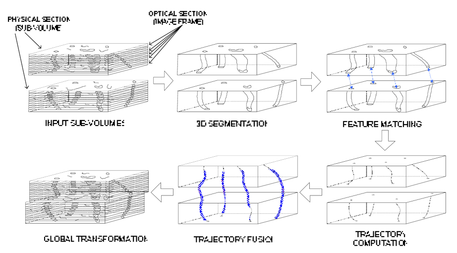
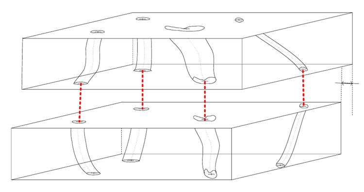
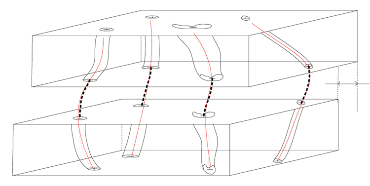
In this paper, we developed a trajectory-based sub-volume alignment method using two trajectory fusion objectives, such as minimum discontinuity across the pair of adjacent sub-volumes and minimum residual of a polynomial fit to corresponding trajectory points from the adjacent sub-volumes. The overall process of the developed techniques is described as follows, and an overview is shown in Figure 1.
Figure 1.
Overview of the trajectory-based alignment.
Perform 3D segmentation to detect all possible closed volumetric segments (e.g., vascular structures) in each sub-volume.
Remove incomplete volumetric segments (e.g., short segments along z-axis).
Find corresponding volumetric segments in two adjacent sub-volumes.
Compute volumetric segment trajectory points by estimating 2D centroids in each 2D frame of a sub-volume.
Determine pairs of alignment control points from two adjacent sub-volumes by fusing corresponding sets of trajectory points.
Estimate parameters of a global alignment transformation model based on the pairs of alignment control points.
2.1 Three-dimensional segmentation
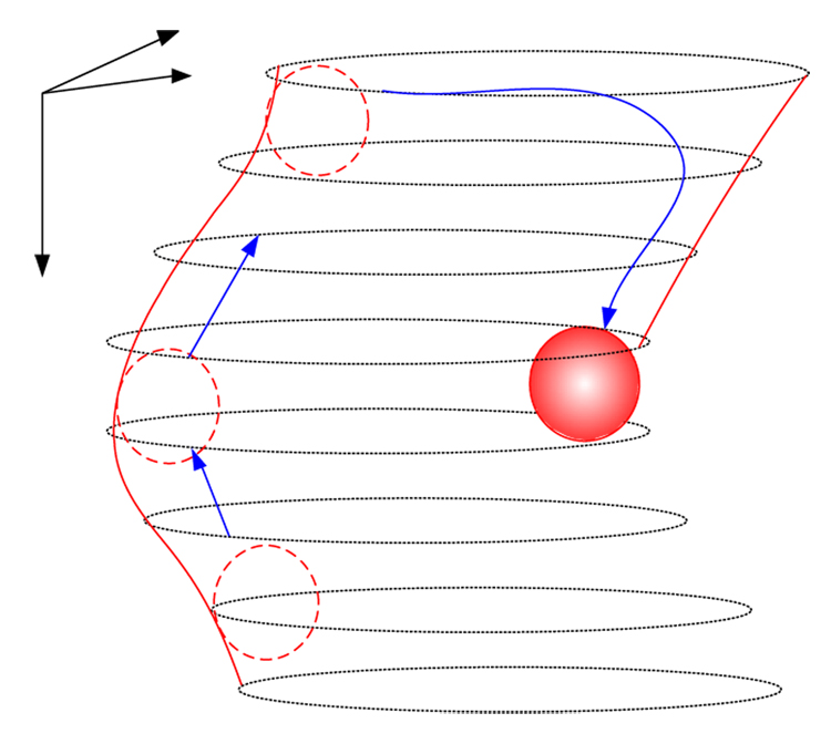
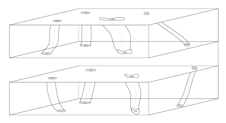
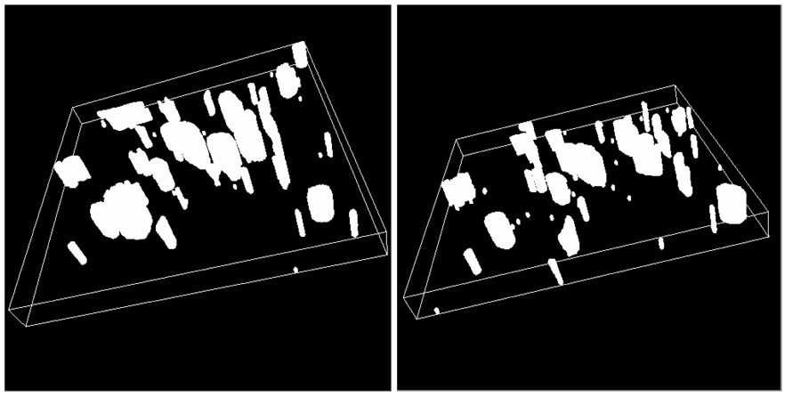
We developed a sphere-based region growing method that can segment out partially closed volumetric segments by extending 2D ball-based segmentation method described in [15]. The volumetric segments in our data correspond to vascular structures. In the absence of artificially inserted fiduciary markers, detecting vascular structures is critical for computer-assisted 3D volume reconstruction including tile mosaicking and sub-volume alignment tasks. The fact that vascular structures are observed as partially closed volumetric segments in CLSM images is caused by photo bleaching or loss (possibly lack) of a fluorescent dye. The developed region growing method can recover vascular regions in those cases when an edge of a color homogeneous closed region is discontinued, an edge is partially destroyed during noise thresholding (especially if a high threshold has to be applied to remove background), or an edge is missing since it lies partially outside of the imaged area. Figure 2 shows an illustration of 3D segmentation by growing interior region of a vascular region using a virtual sphere (ball). Figure 3 illustrates an example of a pair of sub-volumes after 3D segmentation. Features are illustrated with various levels of deformation along the axial direction (depth axis).
Figure 2.
3D segmentation of a volumetric region using a sphere
Figure 3.
An example of a pair of sub-volumes after 3D segmentation
In order to automate the segmentation process, the foreground versus background threshold value and ball diameter parameters must be chosen. The threshold value is usually based on the Signal-To-Noise (SNR) ratio of a specific instrument. It is possible to optimize the threshold value by analyzing the histogram of connected segments after thresholding as a function of the threshold value because a large number of small segments occurring due to speckle noise disappear around the optimal threshold value. The choice of a ball diameter used for connectivity analysis of partially closed volumes is tied to the medical meaning of structures. It requires medical expertise to select structures of interest and analyze their characteristic boundary length and the level of boundary closeness. Thus, we have experimentally chosen the ball diameter by evaluating multiple segmentation outcomes and selecting the diameter that led to a visually determined “meaningful” number of structures.
2.2 Selection of three-dimensional segments
The three-dimensional segmentation method in Section 2.1 outputs a set of volumetric features from a sub-volume. Due to intensity variation and morphological changes of feature structures, such as blood vessels, structures might be partially open. For those structures, 3D virtual sphere may not always stay inside a cylindrical structure, and therefore we remove the corresponding segments by limiting the number of voxels in a volumetric structure. During this operation, large blood vessel features might be undesirably removed. To prevent the removal, we derived the maximum number of voxels based on statistical analysis of all detected volumetric segments. Unusually large features exceeding the voxel count limit will be removed since in general very large features often lead to less accurate centroid locations than small-to–normal sized blood vessels.
Although volumetric features with significant morphological change or bifurcation may be of interest to medical experts, they are not necessarily useful for registration purpose because of their associated high uncertainty of trajectory point locations. These bifurcating features can be filtered out for registration purposes by comparing the interior areas of blood vessel cross sections along z axis. Sudden changes of two-dimensional vascular area and/or centroid location along z-axis are indicators of bifurcation and are filtered out from the set of selected 3D segments.
2.3 Finding corresponding segments
Although our final goal is to co-register a pair of adjacent sub-volumes based on structural trajectories of detected features, it is often simpler to establish correspondence of pairs of trajectories by comparing 2D shapes of features than comparing 3D shapes of features.
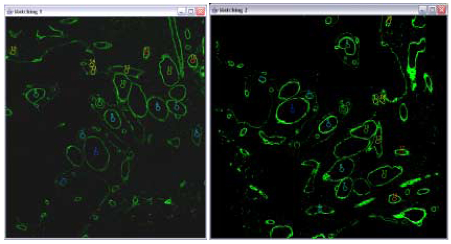
The parameter estimation can be performed using the RANSAC algorithm [16] that randomly evaluates multiple pairs of corresponding pixels. However, in the case of CLSM data, one could use rather a deterministic and computationally simpler method than RANSAC [17]. This method had been evaluated in the past on CLSM data for feature matching [5] and performs sufficiently well. The method establishes feature correspondence by solving the Procrustes problem [18] using two-step matching method, such as Euclidian distance based method followed by vector distance based method. Figure 4 shows an example of result for feature correspondence problem.
Figure 4.
The correspondence outcome from two phases. The left and right images are to be aligned. Overlays illustrate established correspondences between segments that are labeled from 1 through 17. The centroid locations of segments are sorted based on the correspondence error from the smallest error to the largest error.
2.4 Trajectory fusion
The execution of fusion takes two steps. First, we compute trajectory points of a volumetric segment by estimating a set of 2D centroids in each 2D frame of a sub-volume. Next, we fuse pairs of corresponding trajectories from matching segments in adjacent sub-volumes where the matched segments are found according to Section 2.3. The fusion goal of bringing together 3D sub-volumes is achieved by using two different methods, such as extrapolation and residual minimization. These methods take pairs of control points that connect the matching adjacent volume segments and analyze the continuity of the corresponding pairs of trajectories. After completing the fusion of each trajectory, a global transformation minimizing discontinuity of all fused trajectories is computed (described in Section 2.5).
Computing trajectory points of volumetric segments
We define a set of 3D trajectory points derived for the i-th volumetric segment in the k-th sub-volume as follows:
| (1) |
where m is the number of frames (depth) in the sub-volume. The lateral coordinate (x,y) is a centroid location in a frame, and the z coordinate represents the depth (frame index normalized with respect to lateral pixel coordinate system) in a volumetric segment.
Determining pairs of alignment control points at a junction of sub-volumes
This task is achieved by performing trajectory fusion under a set of optimization objectives. The goal of trajectory fusion is to determine pairs of control points to estimate the most accurate global transformation α: R2 → R2 applied to lateral planes (frames) of sub-volumes. In our work, we chose to estimate affine transformation parameters. First, given a set of matching pairs of depth-adjacent trajectories and (i∈ detected features), we compute the modified trajectory by translational offset based on two different fusion approaches (see following sections).
| (2) |
Then, is considered as a set of modified (translated in lateral plane) trajectories that best fuse (connect) the corresponding features in . Next, we compute the global affine transformation α by using all features and the least-squares fit defined as follows:
| (3) |
where n is the number of matching volume features. Finally, we transform a set of images (frame) in the sub-volume k + 1 by the estimated α to create the final aligned sub-volume. We propose two approaches for trajectory fusion denoted as fusion by extrapolation and by polynomial model fitting in following sections.
2.4.1 Fusion by extrapolation
The trajectory fusion by extrapolation is inspired by maximizing connectivity of matching trajectories. Assuming that there are some gaps between adjacent sub-volumes, we extrapolate a pair of points . Then, we compute the translational offset of feature i as follows:
| (4) |
To generate the pair of extrapolated points and , we used two different extrapolation methods such as an end-point duplication and three different degrees of polynomials. First, the end-point duplication is performed by replicating (x,y) coordinate of the adjacent end trajectory points with physical gap Δk between and as follows:
| (5) |
An example of trajectory fusion by end-point duplication is illustrated in Figure 5. Second, the polynomial-based extrapolation is performed by estimating the polynomial functions and with degree γ based on and respectively. To compute the 3D polynomial curve, we estimate a function
| (6) |
where
Next, a pair of extrapolated points is generated as follows:
| (7) |
Figure 5.
Trajectory fusion by connecting end points. T1 denotes the offset after the global affine transformation estimated by the end-point point connection approach.
2.4.2 Fusion by model fitting
The assumption behind the fusion by model fitting is that relatively short trajectory of a blood vessel follows a polynomial curve with degree of less than three (cubic). Although the exact model of the trajectories cannot be defined, we show that maximum three degrees of polynomial fit to the real data quite well based on our experimental results.
First, we define as a residual after fitting γ-degree polynomial function to below:
| (8) |
where and . The coordinate denotes a trajectory point of the trajectory i of the sub-volume k in depth j.
To compute a residual of fused trajectory from a pair of trajectories, we introduce a binary operator . The binary operator performs a simple merging of a pair of trajectories between the sub-volume k and k+1 with a physical gap Δk, e.g., missing frames. Δk is assumed to be a constant for all sub-volumes (typically no more than 3 frame length).
| (9) |
Then the residual of a fused trajectory can be computed as according to Equation (8) and Equation (9).
Next, for each pair of matching trajectories i, we search the translational offset for by minimizing the residual as follows:
| (10) |
An example of trajectory fusion by residual minimization is shown in Figure 6. We limited the search space (U, V), where , to a relatively small pixel neighborhood, e.g., usually less than 10 by 10. It is based on the maximum deviation of the trajectory points from the average location of the trajectory points in x-y plane. Therefore, the computational requirement for residual minimization method is O(n×|U|×|V|) where n is the number of trajectories to be fused. In our experiments, the typical number of matching trajectories was less than 30, and therefore the computational cost for the matching process was negligible in comparison with, for instance, volume segmentation.
Figure 6.
Trajectory fusion by residual minimization of a fitted model. T2 denotes the offset after global affine transformation estimated by the residual minimization approach.
2.5 Global parameter estimation of alignment transformations
Given an affine transformation model α: R2 → R2, the transformation parameters can be estimated by selecting at least three pairs of corresponding points and computing six affine transformation parameters shown in the equation below.
| (11) |
The values (x', y')=α(x,y) are the transformed coordinates of the original image coordinates (x,y) by the affine transformation α(·). The four parameters, a00, a10, a01, and a11, represent a 2 by 2 matrix compensating for scale, rotation and shear distortions. The two parameters, b0 and b1, represent a 2D translation vector. The parameter estimation can be performed either (1) by feature selection method (i.e., selection of three features) based on a compactness measure Error! Reference source not found. or (2) by performing a least-squares fit to all features and solving the over-determined set of linear equations for the six affine transformation parameters.
From the image alignment accuracy viewpoint, selected pairs of segment centroids should be well spatially distributed in the x-y image plane and should not be collinear. If points are close to be collinear then the affine transformation parameters cannot be uniquely derived from a set of linear equations (more unknowns than the number of equations), and hence the alignment is characterized by large errors. If points are locally clustered and do not cover an entire image spatially then the affine transformation is very accurate only in the proximity of the selected points. However, the affine transformation inaccuracy increases with the distance from the selected points, and thus spatially global registration error metrics lead to large alignment errors again. In order to avoid large alignment errors, we have designed a compactness measure that assesses the pairs of matched centroid points in terms of their distribution and collinear arrangement. The compactness measure is defined as the ratio of the entire image area divided by the largest triangular area formed from the control points.
2.6 Evaluation metrics for alignment accuracy
In this section we introduce three evaluation metrics to be used after applying the final global transformation, such as (1) discontinuity magnitude at sub-volume boundary points, (2) overall discontinuity residual, and (3) junction discontinuity residual. The residuals were computed by fitting polynomial curves to multiple sub-volumes after the final global transformation. Developed two methods, i.e., extrapolation and model fitting, were evaluated by these three evaluation metrics, and the results were presented in Section 3.
Metric 1: Discontinuity magnitude at sub-volume boundary points
The overall discontinuity between sub-volumes k and k + 1 is defined as follows:
| (12) |
where the i-th trajectory discontinuity is a Euclidian distance (in lateral plane) of the connecting point pair and generated based on Equation (7). For our experiment, we assumed that trajectories could be modeled by low degree polynomials, and therefore the discontinuity was measured by linear extrapolation at the end points (d(γ=1)(·)).
Metric 2: Overall discontinuity residual after polynomial curve fitting to multiple aligned subvolumes
The discontinuity residual of the γ-degree polynomial model for the Δk physical gap between adjacent sub-volumes can be evaluated according to the equation below:
| (13) |
where is a residual of the i -th feature in the sub-volumes k and k + 1 after merging a pair of trajectories with a binary operator (as shown in Eq. (9)) referring a physical gap Δk between the two sub-volumes. The value n is the number of matching trajectories (features). We assume that sub-volume correspondence is known, for example, and are assumed to be a pair of matching volume features.
Metric 3: Junction discontinuity residual after polynomial curve fitting to multiple aligned sub-volumes
The junction discontinuity residual of the the γ-degree polynomial model for the Δk physical gap between adjacent sub-volumes includes residuals only over the junctions. The definition of the junction discontinuity metric is provided below:
| 14 |
3 Experiments
In this section, we present the experimental materials and the performance evaluations of the proposed trajectory based registration under the evaluation metrics described in Section 2.6. We used four consecutive serial sections of human tonsil tissue samples as described in Section 3.1, applied two different approaches, such as extrapolation and residual minimization, and evaluated results with three alignment accuracy metrics, such as discontinuity magnitude, and overall and junction residuals.
3.1 Material preparation
Formalin-fixed, paraffin-embedded tonsil tissue samples were sectioned at 4 µm thickness. The use of archival human tissue in this study was approved by the Institutional Review Board of the University of Illinois at Chicago. All histological serial sections were examined with a Leica SP2 laser scanning confocal microscope (Leica, Heidelberg, Germany) using the 40× objective with 500 ~ 650 nm excitation wavelength range for the test specimens. Images were stored in tagged information file format (TIFF) with 512 by 512 pixel resolution. One 3D volume was formed from 24 image frames along axial coordinates (z-coordinate or depth) in the same lateral area. Therefore, a sub-volume consists of 512 by 512 by 24 voxels, which is equivalent to 237.92 × 237.92 × 3.74 microns in physical dimension. The green structures represent extravascular matrix patterns (loops) or blood vessels.
3.2 Results
We evaluated the discontinuity magnitude, and overall and junction residuals by considering three variables for trajectory based 3D volume reconstruction from CLSM: (1) polynomial degree γ of centroid trajectories along axial direction (z-axis of the sub-volume), (2) a range of gaps between adjacent sub-volumes Δk, and (3) trajectory fusion approach (extrapolation versus residual minimization). Four consecutive sub-volumes were used for our evaluation, and therefore three pairs of sub-volume registration results are shown. We labeled these four sub-volumes as S1, S2, S3, and S4.
Feature segmentation
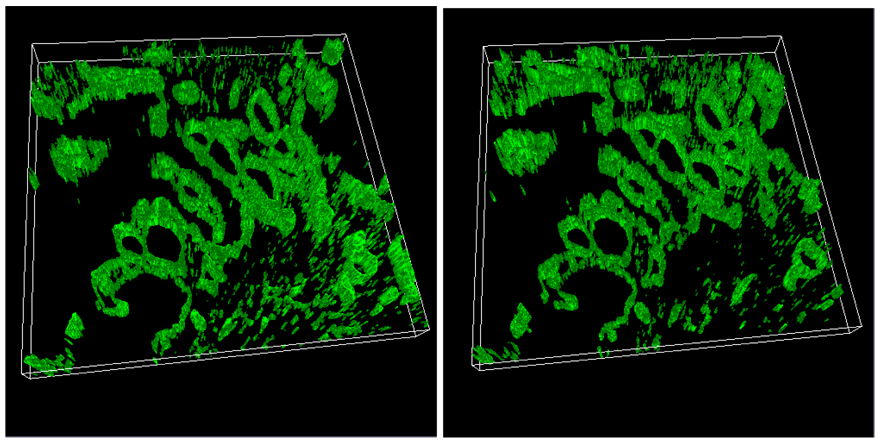
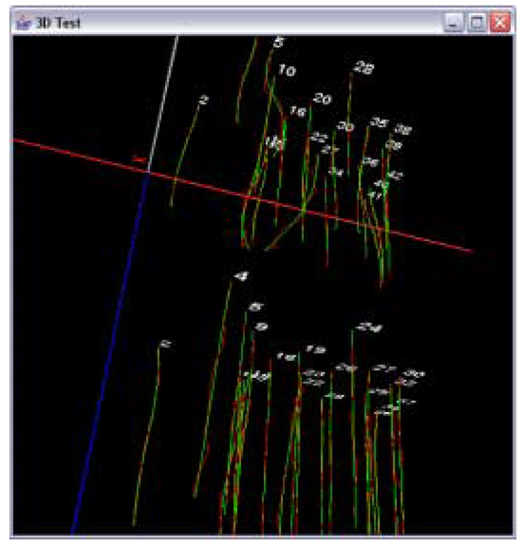
Figure 7 shows an example of a pair of input sub-volumes. The green structures represent extravascular matrix patterns (loops) or blood vessels in human tonsil tissues. Since tonsillar tissues contain plenty of features with closed contours that represent blood vessels, those feature regions are segmented out using 3D ball-based segmentation as described in Section 2.1. Figure 8 shows segmented sub-volumes. As observed in the 3D segmented volumes, we could extract enough number of cylindrical structures where the set of trajectories are to be extracted. Although the centroid locations in a cylindrical structure could be distorted by structural shape changes and/or segmentation accuracy, we assume the major contribution of the centroid location is from the structural trajectory of the blood vessels (cylindrical structures). After acquiring the set of volume features as shown in Figure 8, feature correspondence was established based the automated feature matching method as described in [17]. Next, we computed trajectories and (i ∈ matching features) based on the series of centroids from 2D optical sections in each volume feature. Figure 9 shows an illustration of 3D trajectories for the pair of (S1, S2) sub-volumes. Red line segments represent the actual centroid points, and the green curves indicate polynomial curves with the degree of three. Also notice that the numerical labels on each trajectory show the trajectory correspondences between S1 and S2.
Figure 7.
A pair of CLSM sub-volumes (S1 and S2): (left) sub-volume 1 (upper physical section) and (right) sub-volume 2 (lower physical section).
Figure 8.
Segments obtained by segmenting sub-volumes in Figure 7. Cylindrical structures represent segments of blood vessels in the test specimen.
Figure 9.
A pair of sets of trajectories from adjacent sub-volumes (enhanced range). Numbers indicate the labels of matching trajectories. Red line segments indicate centroids, and green curves indicate a polynomial function with the degree of three.
Trajectory fusion
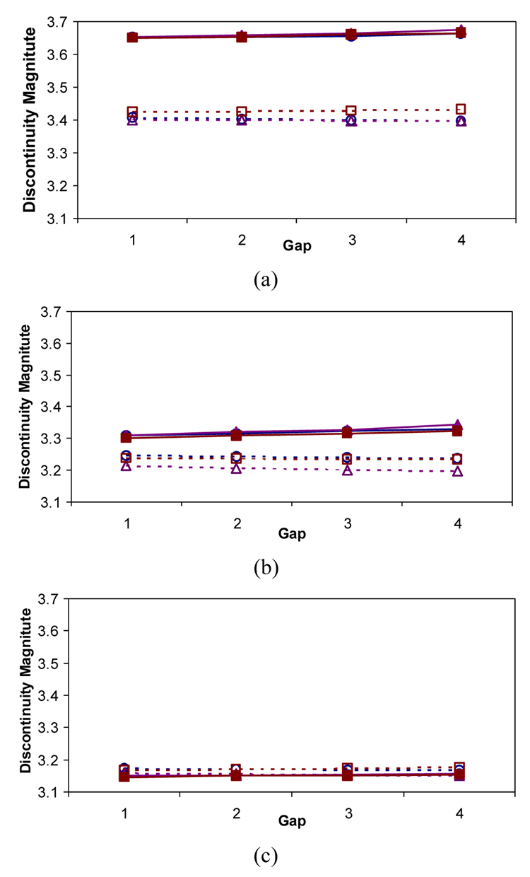
Figure 10 shows the results of trajectory fusion evaluated based on discontinuity magnitude metric (metric 1) using the extrapolation and residual minimization methods. Multiple curves in Figure 10 correspond to linear, quadratic, and cubic models and the results are presented as a function of gaps between a pair of sub-volumes. Based on the results, we arrived to the following two conclusions about the discontinuity metric (metric 1). First, if pairs of sub-volumes are characterized by large physical discontinuities (e.g., S1-S2 has larger physical discontinuity than S3-S4), then the differences between the two methods are more noticeable and the extrapolation method outperforms the residual minimization method. For example, Figure 10 (a) shows not only relatively high absolute value of discontinuities but also large relative differences of discontinuities between the two methods (3.4~3.7 discontinuity range in pixels) in comparison with Figure 10 (b) (3.2~3.4 discontinuity range) and Figure 10 (c) (3.1~3.2 discontinuity range). Second, if trajectories could be described by low degree polynomials then the methods would be relatively insensitive to the polynomial model complexity (e.g., curves in the graph using the same method remain close to each other) and almost independent of a small range of physical gaps.
Figure 10.
Trajectory discontinuity (metric 1) as a function of physical gaps between adjacent sub-volumes: S1 and S2 in (a), S2 and S3 in (b), and S3 and S4 in (c). EX() and RM() refer to extrapolation method and residual minimization method respectively. The extrapolation method is plotted with dotted lines, while the residual minimization method is plotted with solid lines.
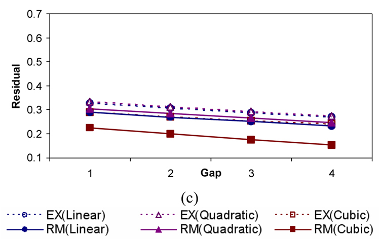
Figure 11 shows the results of trajectory fusion evaluated based on the overall discontinuity residual metric (metric 2) using the extrapolation and residual minimization methods. Our conclusions based on Figure 11 are as follows. First, the residual minimization method always outperforms the extrapolation method for the same degree polynomial models. Second, all trajectory residuals (for all methods and their degrees of polynomial models) decrease as a function of physical gaps between adjacent sub-volumes. Third, the absolute value of trajectory residuals depends more on the degree of polynomial models than on the method type.
Figure 11.
Overall trajectory residual (metric 2) as a function of physical gaps between adjacent sub-volumes: S1 and S2 in (a), S2 and S3 in (b), and S3 and S4 in (c). EX() and RM() refer to the extrapolation and residual minimization methods respectively. The extrapolation method is plotted with dotted lines, while the residual minimization method is plotted with solid lines.
Figure 12 shows the results of trajectory fusion evaluated based on junction residual metric (metric 3). The results are similar to the results in Figure 11 in terms of the trends. The differences are (a) in smaller absolute magnitudes of the residual values due to the exclusion of parts of the residuals from metric 3 that are present in metric 2, and (b) in clustering of the results obtained from extrapolation and residual minimization methods.
Figure 12.
Junction trajectory residual (metric 3) at junctions as a function of physical gaps between adjacent sub-volumes: S1 and S2 in (a), S2 and S3 in (b), and S3 and S4 in (c). EX() and RM() refer to the extrapolation and residual minimization methods respectively. The extrapolation method is plotted with dotted lines, while the residual minimization method is plotted with solid lines.
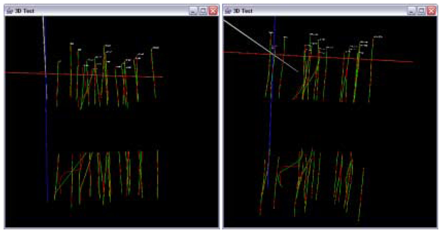
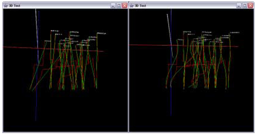
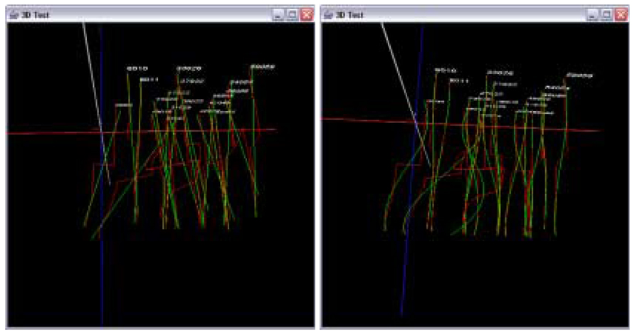
Figure 13 shows 3D trajectories from the sub-volumes S1 and S2 before trajectory fusion (enhanced range). Figure 14 and Figure 15 show the results of the data in Figure 13 after trajectory fusion using extrapolation and residual minimization methods respectively with linear and cubic polynomial models.
Figure 13.
Visualization of extracted trajectories from S1 and S2 assuming the gap equal to one frame depth. Curve fitting results with a linear model (left) and with a cubic model (right).
Figure 14.
Visualization of trajectory fusion using the extrapolation method with gap equal to one (enhanced range). Fused trajectories with a linear model (left) and a cubic model (right).
Figure 15.
Visualization of trajectory fusion using the residual minimization method with gap equal to one (enhanced range). Fused trajectories with a linear model (left) and a cubic model (right).
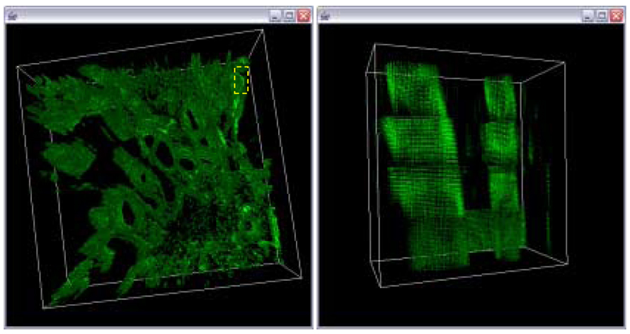
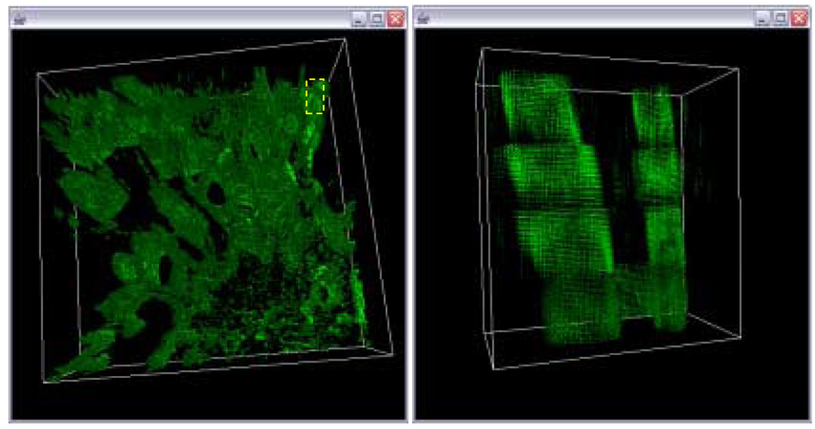
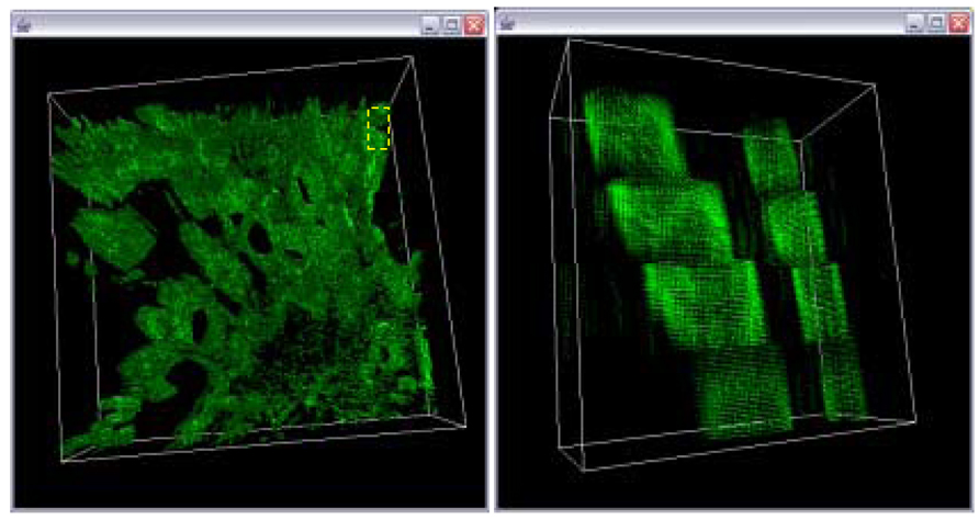
Based on the trajectory fusion results, we computed the optimized global affine transformation, and they are shown in Figure 17 and Figure 18. For visual comparison purpose, we show the 3D image and a side view of the reconstructed volumes in a sub-region without any trajectory fusion (see Figure 16), with extrapolation-based trajectory fusion (see Figure 17), and with residual minimization-based trajectory fusion method (see Figure 18). Based on the visual verification, one could observe that the discontinuities between adjacent sub-volumes are much higher without trajectory fusion than with any of the trajectory fusion methods. How to select an appropriate method was not studied in this work, and the discussion of this issue is provided in Section 4.
Figure 17.
Final 3D volume after trajectory fusion with extrapolation for gap equal to one and a linear model A magnified view of the sub-area in the left image delineated by the yellow box.
Figure 18.
Final 3D volume after trajectory fusion with residual minimization for gap equal to one and a cubic model (left). A magnified view of the sub-area in the left image delineated by the yellow box.
Figure 16.
Final 3D volume without trajectory fusion for gap equal one (left). A magnified view of the sub-area in the left image delineated by the yellow box.
4 Discussion
In this section, we discuss first how an end-user could select the most appropriate fusion method and polynomial degree (model complexity). Next, we discuss the performance evaluation methodology.
Method and Model Selection
In terms of the fusion method selection, the choice could be driven by weighting application specific priorities, such as a continuity of matched trajectories at the sub-volume border or a smoothness of matched trajectories within the two adjacent sub-volumes. These decisions can be guided by designing a cost function for a hybrid fusion method. In terms of the polynomial degree selection, the polynomial degree (model complexity) should be chosen based on a priori knowledge about medical structures and their corresponding feature trajectories. It is recommended to avoid over-fitting by studying medical structures of interest.
For example, if there exists a solid understanding of 3D trajectory models of medical structures, then the residual minimization method would be preferred. Otherwise, the extrapolation method would be recommended with the goal to improve continuity of adjacent sub-structures (features). Yet another possibility of trajectory fusion may be a combination of the proposed two methods. After computing the global adjustments Uextrapolation and Uresidual_minimization in a lateral plane (where , and ), the final hybrid adjustment Uhybrid could be calculated by weighting Uextrapolation and Uresidual_minimization such as , where λ is a weighting coefficient in [0,1].
Performance Evaluation Methodology
In this work, we presented our quantitative evaluation metrics and visual comparisons to assess morphological smoothness. However, we did not show performance evaluations based on comparisons with ground truth transformations because it is extremely difficult to create ground truth data. We have attempted to devise three simulation methodologies to simulate realistic CLSM sub-volumes with known (ground truth) alignment parameters. First, we split one sub-volume into two adjacent pieces that would simulate tissue sectioning. Since splitting a series of images does not introduce any geometrical distortion, the ground truth parameters are known to be a unit transformation and could be compared with the optimized transformation based on our developed methods. However, we were unsuccessful with this simulation approach because physical sectioning was excluded from the simulation, i.e., a simple end-point connection gives the best alignment result. Second, to simulate distortions due to physical sectioning, we tried to apply in the neighborhood of two connecting sub-volumes to introduce data driven trajectory distortion following an exponential model (empirically observed in several serial sections). Nonetheless, we discovered that it is almost impossible to recover the model parameters of the physical distortion introduced by sectioning. Third, we simulated the physical sectioning by swapping the depth locations of the split volume as described in the first simulation approach. For example, the images labeled from 1 to 24 are split into two image sets, such as 1~12 and 13~24, and then the images are reordered as 13, …, 24, 1,…,12. This simulation scenario is motivated by the fact that the both connecting z-frames of a sub-volume are naturally distorted by physical sectioning. We concluded that the main problem with this type of simulation was the change of the trajectory structure that would not correspond to realistic morphological changes in a specimen. As a result, we evaluated our trajectory-based registration performance based on visual smoothness as most medical experts would do currently, in addition to the evaluations by the two metrics, such as the discontinuity and trajectory residual metrics.
5 Conclusion
We addressed the problem of 3D volume reconstruction from depth adjacent CLSM sub-volumes by estimating an optimal global image transformation which preserves morphological smoothness of medical structures inside of the reconstructed 3D volume. To preserve morphological smoothness of the reconstructed 3D medical structures, we defined three metrics for morphological discontinuity (discontinuity magnitude at sub-volume boundary points and overall and junction discontinuity residuals after polynomial curve fitting to multiple aligned sub-volumes), and then minimized the metrics across adjacent sub-volumes and all salient structures. Our experimental results demonstrate significantly improved morphological smoothness of medical structures evaluated visually or by the defined metrics when applied to human tonsil tissues.
The main contributions of this work are in (1) the presentation of two novel registration optimization methods using trajectory fusion, and (2) the three quantitative evaluation metrics for assessing morphological smoothness of the adjoined trajectories. In addition, our developed 3D volume registration using trajectory fusion has not yet been applied in any application domain in the past and our particular application to CLSM data was successfully demonstrated in this work.
Our future research will extend the registration framework by including other segmented features than just the centroid points forming trajectories. In addition, we will investigate global registration approaches with large data sets. For example, in order to explore the effects of global bundle adjustment with large data sets, one has to analyze theoretical limitations of the underlying structures and consider the practical challenges of data preparation. (preparation time, data quality and cost). The global bundle adjustment applied to all affine pairwise estimates would be feasible in theory if the trajectory would be persistent. In this case, persistent trajectory refers to a cylindrical structure found in all frames across all sub-volumes without significant morphological changes (e.g., bifurcation) and intensity changes (e.g., fluorescent fading). Based on our current understanding of the medical structures, there would be a need to collect data and study the persistence of trajectories before applying the global bundle adjustment.
6 Acknowledgement
This material is based upon work supported by the National Institute of Health under Grant No. R01 EY10457. The on-going research is collaboration between the Department of Pathology, College of Medicine, University of Illinois at Chicago (UIC) and the Image Spatial Data Analysis Group, National Center for Supercomputing Applications (NCSA), University of Illinois at Urbana-Champaign (UIUC). We would like to especially acknowledge Dr. Robert Folberg and Dr. Amy Lin from the Department of Pathology at UIC for providing the experimental data for our work and introducing us to the problems of 3D volume reconstruction from CLSM images. We would like to thank to the anonymous reviewers for their valuable comments on the manuscript draft.
Footnotes
Publisher's Disclaimer: This is a PDF file of an unedited manuscript that has been accepted for publication. As a service to our customers we are providing this early version of the manuscript. The manuscript will undergo copyediting, typesetting, and review of the resulting proof before it is published in its final citable form. Please note that during the production process errors may be discovered which could affect the content, and all legal disclaimers that apply to the journal pertain.
Contributor Information
Sang-Chul Lee, Email: sclee@ncsa.uiuc.edu.
Peter Bajcsy, Email: pbajcsy@ncsa.uiuc.edu.
7 References
- 1.Michiel M. Introduction to Confocal Fluorescence Microscopy. second edition. SPIE press; 2006. [Google Scholar]
- 2.Stevens J. Introduction to Confocal Three-Dimensional Volume Investigation, in three-dimensional confocal microscopy: volume investigation of biological systems. Academic press; 1994. pp. 3–27. [Google Scholar]
- 3.Trochim W. The Research Methods Knowledge Base, 2e1. Cornell University; 2001. http://www.socialresearchmethods.net/kb/statrd.htm. [Google Scholar]
- 4.Bajcsy P, Lee S-C, Clutter D. Supporting Registration Decision during 3D Medical Volume Reconstruction. SPIE International Symposium in Medical Imaging.2006. [Google Scholar]
- 5.Bajcsy P, Lee S-C, Lin A, Folberg R. 3D Volume Reconstruction of Extracellular Matrix Proteins in Uveal Melanoma from Fluorescent Confocal Laser Scanning Microscope Images. Journal of Microscopy, Blackwell Synergy. 2006 doi: 10.1111/j.1365-2818.2006.01539.x. [DOI] [PMC free article] [PubMed] [Google Scholar]
- 6.Benson D, Bryan J, Plant A, Gotto A, Smith L. Digital Imaging fluorescence microscopy: Spatial heterogeneity of photobleaching rate constants in individual cells. J. Cell Biol. 1985;100:1309–1323. doi: 10.1083/jcb.100.4.1309. [DOI] [PMC free article] [PubMed] [Google Scholar]
- 7.Jungke M, Seelen VW, Bielke G, Meindl S, et al. A system for the diagnostic use of tissue characterizing parameters in NMR-tomography. Proc of Info. Proc. in Med. Imaging, IPMI'87; 1987. pp. 471–481. [Google Scholar]
- 8.Chan H, Chung A. Efficient 3D-3D Vascular Registration Based on Multiple Orthogonal 2D Projections. Second International Workshop on Biomedical Image Registration, (WBIR’03) 2003:301–310. [Google Scholar]
- 9.Kang J, Cohen I, Medioni G. Continuous multi-view tracking using tensor voting. IEEE Workshop on Motion and Video Computing; Orlando, Florida. 2002. Dec 5–6, [Google Scholar]
- 10.Caspi Y, Irani M. A Step towards Sequence-to-Sequence Alignment. IEEE Computer Society Conference on Computer Vision and Pattern Recognition (CVPR'00); 2000. p. 2682. [Google Scholar]
- 11.Leclerc YG, Zucker SW. The Local Structure of Image Discontinuities in One Dimension. IEEE Transactions on Pattern Analysis and Machine Intelligence; 1987. pp. 341–355. [DOI] [PubMed] [Google Scholar]
- 12.Leclerc YG. Capturing the Local Structure of Image Discontinuities in Two Dimensions. Proceedings of the IEEE Computer Society Conference on Computer Vision and Pattern Recognition; San Francisco, California. 1985. Jun, pp. 34–38. [Google Scholar]
- 13.Pavlidis T, Liow YT. Integrating region growing and edge detection. IEEE Trans. Pattern Analysis Machine Intellig.; 1990. Mar., pp. 225–233. [Google Scholar]
- 14.Le Moigne J, Tilton JC. Refining Image Segmentation by Integration of Edge and Region Data. IEEE Transactions on Geoscience and Remote Sensing; 1995. May, pp. 605–615. [Google Scholar]
- 15.Lee S-C, Bajcsy P. Feature based Registration of Flourescent LSCM Imagery. Proc. of SPIE International Symposium in Medical Imaging.2005. [Google Scholar]
- 16.Fischler MA, Bolles RC. Random Sample Consensus: A Paradigm for Model Fitting with Applications to Image Analysis and Automated Cartography. Comm. of the ACM. 1981;Vol 24:381–395. [Google Scholar]
- 17.Lee S-C, Bajcsy P. Automated feature-based alignment for 3D volume reconstruction of CLSM imagery. Proceedings of SPIE Conference on Medical Imaging; San Diego, CA. 2006. Feb 11–16, p. 6144-105. [Google Scholar]
- 18.Dorst L. First order error propagation of the procrustes method for 3D attitude estimation. IEEE Trans. Pattern Anal. Mach. Intell.; 2005. pp. 221–229. [DOI] [PubMed] [Google Scholar]


