A Dimensionality Reduction Technique for Efficient Time Series Similarity Analysis

Abstract

We propose a dimensionality reduction technique for time series analysis that significantly improves the efficiency and accuracy of similarity searches. In contrast to piecewise constant approximation (PCA) techniques that approximate each time series with constant value segments, the proposed method--Piecewise Vector Quantized Approximation--uses the closest (based on a distance measure) codeword from a codebook of key-sequences to represent each segment. The new representation is symbolic and it allows for the application of text-based retrieval techniques into time series similarity analysis. Experiments on real and simulated datasets show that the proposed technique generally outperforms PCA techniques in clustering and similarity searches.

1. INTRODUCTION

The problem of efficient retrieval of similar time series in large databases has received considerable attention by the data mining community because of its application to many fields, including medicine, meteorology, economics, and astrophysics. A broad overview of the data mining approaches that have been proposed to measure the similarity and dissimilarity of time series is provided in [1, 2] and a more specific overview on time series databases can be found in [3, 4].

Queries for the retrieval of similar time series fall into two groups: range queries and nearest neighbor queries. A range search may be stated as follows: Given a query series q, a database S of N series, S₁, S₂,…, S_N, a distance measure D and a tolerance threshold ε, find the set of time series R in S that are within distance ε from q. More precisely find: R = {S_i ∈ S | D(q,S_i)≤ ε}. For a nearest neighbor search, no threshold is given and the closest neighbors of the query series are found. Another classification of time series similarity search problems is based on the relation of the length of the query series to that of the series in S. In the whole matching problem, the series in S and the query have the same length. In the subsequence-matching problem, we seek all possible subsequences of elements of S that match the query series.

To compare two given time series, a suitable measure of similarity must be used. This is not a trivial problem, and as a result, many approaches and techniques have been suggested in the past decade [1, 2, 5–15]. The plain Euclidean distance approach for comparing time series takes linear time in the length of the series. For some applications in large time series databases it may not be useful. Promising techniques include those that are based on reduction of dimensionality of the original series and use of multidimensional indexing (e.g., spatial access methods such as R-trees [16]). In such cases, the series can be represented as multidimensional vectors and similar series can be retrieved in sub-linear time.

The reduction of the original series’ dimensionality is crucial because spatial access methods only perform well when the number of dimensions is low (typically below 15). The solution to extract a signature from each time series and to index the signature space was originally proposed by Faloutsos et al [8, 9, 16]. To guarantee completeness (i.e., no false dismissals) the admissibility criterion that the distance function used in the signature space must underestimate the true distance measure (bounding lemma) was also proposed [9].

Agrawal et al [5] introduced the F-index, a time series signature extracted from the frequency domain. The strongest coefficients of a Discrete Fourier Transform were proposed to represent most real time series. This method was proposed to solve the whole-sequence matching problem. The ST-index was later proposed by Faloutsos et al [9] to allow subsequence matching. In this approach, for each time series in the database and for each position in the series, the authors propose the use of a sliding window w over the data sequence and to extract its features. This results in a trail in signature space. They then efficiently divide such trails into sub-trails that are represented by their Minimum Bounding Rectangles (MBRs). Finally, the MBRs are stored in a spatial access index structure. In order to search for subsequences similar to a query q of length w, one simply has to look up all MBRs that intersect a hypersphere with radius ε around the signature point q.

Landmark models have also been introduced to solve the problem [14]. In this case, points of “great importance” such as local maxima or minima are identified as landmarks. The landmarks offer a signature that is usually invariant to a subset of the following transformations: time-warping, shifting, uniform amplitude scaling, non-uniform amplitude scaling, uniform time scaling, etc. Other techniques for comparing sequences to databases that use dynamic programming and suffix trees [17] to avoid duplicate calculations have been introduced [7, 18]. The goal is to reduce extra calculations using suffix trees in order to speed up the comparison of sequence prefixes.

Another approach for efficient similarity searches on time series is based on piecewise constant approximation (PCA), also known as piecewise aggregate approximation (PAA). Yi and Faloutsos [15] and Keogh et al [11] proposed to divide each series into k segments of equal length and to use the average value of each segment to represent the latter. There are several advantages to this transform: it is very fast and easy to implement, the signature can be used with arbitrary L_p norms, and the index can be built in linear time. In addition, the representation can be used with a weighted Euclidean distance where each segment of the sequence has different weight. Keogh et al. [2] have also proposed an Adaptive Piecewise Constant Approximation where the segments can be of variable length and offer a more effective compression than PCA.

Recently, a symbolic PAA technique called Symbolic Aggregate approXimation (SAX) was introduced [19]. This approach, by making the assumption that the values in normalized time series have highly Gaussian distribution, introduces standard “breakpoints” to make the time series discrete.

As dimensionality reduction has become more and more important for fast similarity searches in large time series databases, we focus on achieving a representation of reduced dimensionality. Our work is motivated by the observation that the mean value that is being used to approximate each equal length segment in PCA is the best one can do for a piecewise approximation if there is no prior knowledge about the data or a method needs to be independent of the data. This follows from the basic Shannon source coding theorems [6,9]. The mean value is the best representative of all points when the transmission rate is zero (i.e., we do not transmit anything). Although the method proposed here is also based on the segmentation of a sequence, it extends PCA by allowing for a more flexible approximation of each segment using ideas from data compression. In particular, it uses the vector quantization technique to effectively represent a long time series with a representation of much lower dimensionality (where segments are represented by symbols or codewords). The proposed symbolic representation potentially allows for the application of text or string based retrieval techniques into the time series similarity analysis. In addition to a comparable level of complexity in regards to other methods, the proposed approach demonstrates several advantages, including a closer approximation of original time series, a higher accuracy in time series similarity search, an ability to support flexible queries with variable length, and the allowance of flexible distance measures including the weighted Euclidean distance.

The rest of the paper is organized as follows: Section 2 provides background information on time series similarity measures and preliminaries on Vector Quantization. Section 3 introduces the framework of the proposed dimensionality reduction technique--Piecewise Vector Quantized Approximation (PVQA). Experimental results are presented in Section 4. Directions for future work and concluding remarks are presented in Section 5.

2. PRELIMINARIES

For clarification, this section provides descriptions of various concepts and definitions used in this paper. Table 1 gives a brief description of the notation we use.

Table 1.

Symbols

X	Original time series, X = x1, x2,…, xn of length n
X′	Encoded form of the original time series $X^{\prime }=x_1^{\prime },x_2^{\prime },\dots ,x_w^{\prime }$
N	Number of time series in the dataset
D	The Euclidean distance between two time series
w	The length of the encoded form of a time series
l	Length of each codeword
C	Codebook, a set of codewords {c1, c2,…, cs}
s	Size of the codebook

We start with the definitions of a time sequence and its subsequences:

Definition 1

Time Sequence

A sequence (ordered collection) of real values X = x₁, x₂,…, x_n.

Definition 2

Subsequence

Given a time sequence X = x₁, x₂,…, x_n, we say that x_k, x_k,…, x_km is a subsequence of X with length m if 1 ≤ k₁ ≤ k₂ … ≤ k_m ≤ n.

In the above definitions n can be very large.

In similarity analysis, we need to define a measure for the similarity or dissimilarity (distance) between two time series. The most popular measure used in various applications is the Euclidean Distance. Given two time series, X = x₁, x₂,…x_n, Y = y₁, y₂,…y_n, their distance, D, is defined in general as $L_p={({\displaystyle \sum _{i=1}^n}\mid x_i-y_i{\mid }^p)}^{1/p}$ for an L_p norm (when p = 2, the distance L₂ stands for the Euclidean distance).

The simplest and most obvious way to evaluate the similarity (or dissimilarity) among time series is to compute the Euclidean distance directly, in other words, on the original series. For a small dataset this may be feasible. However, for large data sets efficiency is a problem, since the time complexity is O(N*n), where n is the number of features that need to be represented for each time series and N is the number of time series in the dataset. In order to compute similarity and index efficiently, many techniques for dimensionality reduction such as the Discrete Fourier Transform (DFT), the Discrete Wavelet Transform (DWT) and the Piecewise Constant Approximation (PCA), have been suggested.

In this paper, we introduce a new piecewise approach for representing a time series and calculating similarity based on Vector Quantization (VQ) (A preliminary result of this work was presented in [20].). VQ is widely used in signal compression and coding; it is a lossy compression method based on principle block coding [21]. Recently, it has been applied to deal with the problems of time series forecasting and segmentation [22, 23]. According to Shannon’s theory, coding systems can perform better if they operate on vectors or groups of symbols rather than on individual symbols. The design of a VQ-based system mainly consists of three steps:

• Constructing a codebook from a set of training samples;

• Encoding the original signal with the indices of the nearest code vectors in the codebook;

• Using an index representation to reconstruct the signal by looking up in the codebook.

In VQ a codeword (or code vector) is used to represent a number of similar vectors. More precisely, a vector quantizer Q of dimension n and size s is a mapping: Q: ℜⁿ→C from a vector or a point in n-dimensional Euclidean space, ℜⁿ, to a finite set C = {c₁,c₂,…,c_s}, the codebook, containing s output or reproduction points c_i∈ℜⁿ, called codewords. Associated with every vector quantizer with s codewords is a partition of ℜⁿ into s regions or cells R_i for i∈J≡{1,2,…,s} where R_j = {x∈ℜⁿ: Q(x) = c_i}. A distortion function is used to evaluate the overall quality degradation due to approximation of a vector by its closest representative from a codebook. For the mean-squared error distortion function d(x,c_i) between an input vector x and a codeword c_i, an optimal mapping should satisfy two conditions: (a) the nearest neighbor condition and (b) the centroid condition.

• Nearest neighbor Condition

For a given codebook, the optimal partition R = {R_i: i = 1,…,s} satisfies:

$$R_i=\{x:d(x,c_i)\le d(x,c_j);\forall j\}$$

where c_i is the codeword representing partition R_i. Given a point x in the dataset, the encoding function for x, Encoding(x) = c_i only if d(x,c_i) ≤d(x,c_j) ∀j.

• Centroid condition

For a given partition region R_i (i = 1,…,s), the optimal reconstruction vector (codeword) satisfies: c_i = centroid(R_i) where the centroid of a set R = {x_i: i = 1,…|R|} is defined as:

$$\mathit{centroid}\hspace{0.17em}(R)=\frac{1}{\mid R\mid }\sum _{i=1}^{\mid R\mid }{x}_i$$

These two conditions are used by an iterative procedure, the generalized Lloyd algorithm [24, 25], to produce a “locally optimal” codebook from a training set. In the following section we show how we use VQ to approximate the original series and perform similarity searches using the new representation.

3. PIECEWISE VECTOR QUANTIZED APPROXIMATION

We propose to reduce the dimensionality of time series data by applying VQ on segments of the time series. The proposed method, called Piecewise Vector Quantized Approximation (PVQA), allows a time series X of arbitrary length n to be represented with a time series of length w where w ≪ n. For the encoding, every series is decomposed into w subsequences each of length l (length of the codeword). For each subsequence, the closest, based on a distance measure, entry in the codebook (codeword), is then found and the corresponding index is stored. Thus, the new representation of a time series is a vector of indices to codewords.

In order to create the codebook, each time series in a training set is partitioned into w segments, each of length l. These segments form the samples used to train the codebook. After training, each codeword in the codebook stands for a key-sequence, which is an approximation for a certain group of subsequences of length l. All the time series are then encoded using the codebook. When a query series is to be processed, it is first encoded using PVQA, and its similarity to other series is computed based on the encoded representations of both the query and the time series in the database. Next we present in detail the codebook generation process, the time series encoding using the codebook, the proposed distance measures, and analyze the space and time complexity of the approach.

3.1 Codebook Generation

In order to obtain the key-sequences and build the codebook, we apply the Generalized Lloyd Algorithm (GLA), which is a variation of k-means clustering. Here, we present this well-known algorithm for generating a codebook of size s based on a training set T of time series.

The GLA starts with an initial codebook and repeats the Lloyd iteration in which the two conditions for optimality are used sequentially, i.e., given a codebook (created in the previous iteration), the optional partition of the space ℜⁿ is found using the nearest neighbor condition, and given a partitioning, the codebook is updated using the centroid condition. The distortion function between each vector and its nearest codeword is then calculated. This process repeats until the fractional drop of the distortion between two consecutive iterations becomes smaller than a given threshold. The convergence of the process is guaranteed; from the necessary conditions for optimality (presented in Section 2) follows that each application of the Lloyd iteration must either reduce or leave unchanged the average distortion [21]. The particular version of GLA we use requires a partition split mechanism to solve the initial codebook generation problem. The algorithm starts with a codebook containing only one codeword -- the centroid of the whole data set. In each repetition and before the application of the Lloyd iteration, it splits all cells and doubles the number of codewords from the previous iteration. In Fig. 1 we present a codebook of key-sequences constructed by the proposed technique for a dataset (Control Chart [26]) that we examine in Section 4.

Fig. 1.

An example of a codebook of key-sequences

The quality of the codebook obviously affects the performance of a vector quantizer, thus it is important to obtain a good codebook. During the training process, the codebook keeps being updated until a certain optimization condition is satisfied. This condition is often the minimization of a distortion measurement d(x, c_i) (e.g., the mean squared error) between a training sample x and its corresponding codeword c_i, or the fractional drop of the distortion becoming less than a given threshold. Usually the quality of a codebook is considered poor when the average of d(x, c_i) is above a given threshold. Although it is possible to reduce the expected distortion by increasing the number of codewords, the computation and storage expenses will also increase at the same time. So, there is a tradeoff between quality and cost.

In this paper, we make an implicit assumption that the data sources are stationary. Under such circumstances, the distribution of the training data is representative of the universal data space. It is then reasonable for us to train a fixed-rate (i.e., fixed number of codewords) vector quantizer with PVQA. As shown in section 4.1, we can obtain satisfying results with queries from outside the training dataset.

It is possible, however, that the performance of PVQA will be deteriorated when the data sources become non-stationary. An adaptive-VQ (AVQ) algorithm can be employed to address this issue. The fundamental idea of an AVQ algorithm is to keep the statistics of the data and update the codebook progressively. It can be either fixed-rate (with a fixed number of codewords) or fixed-distortion (with varying number of codewords). Interested readers are encouraged to check [27] for a comprehensive survey of adaptive vector quantization.

3.2 Time Series Encoding

Once the codebook is constructed, we acquire a new representation of each time series in the dataset. In the encoding phase, PVQA partitions a time series X into w equal size segments each of length l and represents X in a w-dimensional space with a vector $X^{\prime }=x_1^{\prime },x_2^{\prime },\dots ,x_w^{\prime }$. Given a codebook C = {c₁,c₂,…,c_s} consisting of s codewords (where s is an arbitrary integer greater than on equal to 2), each segment of X is replaced with the most similar codeword from the codebook. Formally, the i-th element of X′ is:

$$x_i^{\prime }=\underset{k}{argmin}(\text{D}(se{g}_i,c_k);\hspace{0.17em}k=1,\dots ,s)$$

where seg_i is the i-th segment in X, D is a distance measure, and c_k is the k-th codeword of the codebook C. With each x̄_i being an index to a codeword, an approximation of X is achieved by concatenating the codewords corresponding to each x′_i, i = 1,…,w. For each codeword, c_k, that is used to represent a segment the corresponding index k is stored. Fig. 2 shows an original time series (from the Control Chart dataset that we examine in Section 4) and its reconstruction given a certain codebook (w = 6, s = 16) by concatenating the corresponding codewords. For comparison, we also show the reconstruction using PCA. Note that the proposed representation can approximate the original time series arbitrarily closely depending on the size of the codebook and the number of segments. (A more detailed treatment is presented in Section 3.3.) PCA (or PAA) can also approximate the original series arbitrarily closely but does not have the same flexibility as PVQA; PCA accomplishes this by reducing the segment size only.

Fig. 2.

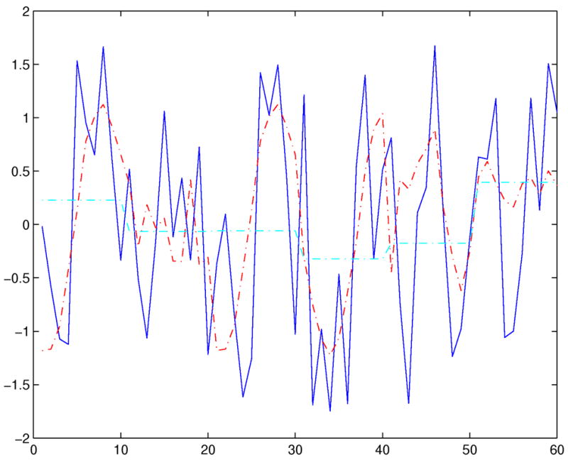
A time series and its reconstructions using PVQA and PCA.

3.3 Distance Measures

PVQA compresses the time series by forming a new representation with a much smaller dimensionality. Here, we consider a distance measure that is appropriate for this new representation. In the domain of time series, a popular distance measure is the Euclidean distance. Recall that for a time series X and a query series Q, both of length n, the Euclidean distance is defined as: $D(X,Q)=\sqrt{{\displaystyle \sum _{i=1}^n}{(q_i-x_i)}^2}$

The distance between two time series is shown graphically as the shaded area in Fig. 3. Calculating the distance is simply the process of computing this shaded area. This process is time-consuming in the case that the two time series are of high dimensionality. However, after encoding the time series using the codebook created by PVQA, the dimensionality is already significantly reduced. Moreover, due to the use of the same codebook for all time series, the computation of the distance for every pair of time series is simplified. One can pre-compute a distance matrix and search it for the distance between each pair of codewords.

Fig. 3.

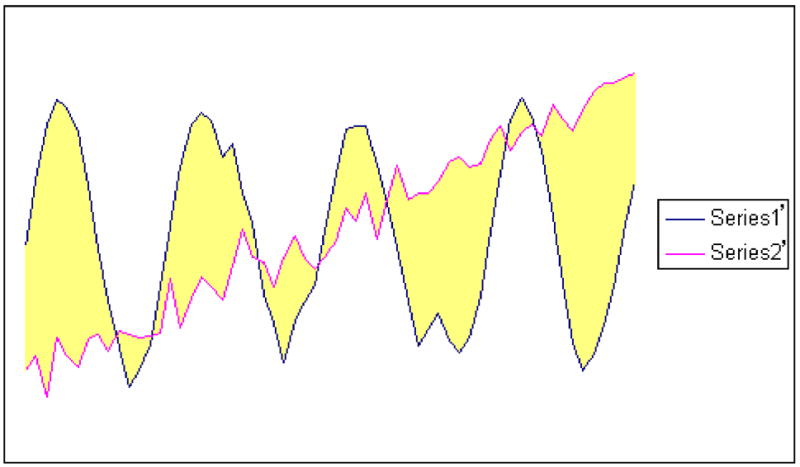
(a) Distance between two original time series (from Control Chart dataset), and (b) distance between the PVQA reconstructions of the two time series (w = 6, s = 16)

After encoding using a codebook, a time series X in the database is represented by a series $X^{\prime }=x_1^{\prime },x_2^{\prime },\dots x_w$, and correspondingly a query series Q is represented as $Q^{\prime }=q_1^{\prime },q_2^{\prime },\dots ,q_w^{\prime }$. Each $x_i^{\prime }$ and $q_i^{\prime }$ (1 ≤ i ≤ w) is an index corresponding to a codeword of the codebook. Since the approximate representation of a time series X or Q is the concatenation of all the codewords corresponding to $x_i^{\prime }$ or $q_i^{\prime }$, we can sum up the distance between each pair of ( $x_i^{\prime },q_i^{\prime }$) and get a rough distance between the two time series:

Definition 3

Rough distance

For two time series X and Q, whose PVQA encoding representation is X′ = x′₁,x′₂, …x′_w and Q′ = q′₁,q′₂, …q′_w, respectively, their rough distance is defined as:

$$\text{RoughDist}(X,Q)=\sqrt{\sum _{i=1}^w{(D(x_i^{\prime },q_i^{\prime }))}^2}$$

Fig. 3 shows two time series and their reconstructions. We observe that since the main characteristics of each series have been kept after reconstruction, their distance can also be approximated with the distance between the two reconstructions.

For a given codebook that consists of a fixed number, s, of codewords, the distance between any two codewords can be pre-computed and stored in a matrix (dist_matrix):

$$\mathit{dist}\_\mathit{matrix}=\left[\begin{array}{lllll}0\hfill & d_{12}\hfill & d_{13}\hfill & \dots \hfill & d_{1s}\hfill \\ d_{21}\hfill & 0\hfill & d_{23}\hfill & \dots \hfill & d_{2s}\hfill \\ d_{31}\hfill & d_{32}\hfill & 0\hfill & \dots \hfill & d_{3s}\hfill \\ \hfill & .\hfill & .\hfill & .\hfill & \hfill \\ d_{s1}\hfill & d_{s2}\hfill & d_{s3}\hfill & \dots \hfill & 0\hfill \end{array}\right]$$

The space complexity is O(s²). The time complexity for building the codebook is discussed later. The time complexity of computing the rough distance between two time series is O(w). Using the precomputed distance matrix, dist_matrix, the definition of RoughDist can be rewritten as:

$$\text{RoughDist}(X,Q)=\sqrt{\sum _{i=1}^w{(d_{x_i^{\prime }{q}_i^{\prime }})}^2}$$

With prior knowledge of the dataset, the rough distance can approximate the true (Euclidean) distance arbitrarily closely based on the parameters s and w.

Let us now evaluate the distance we just introduced. Note that in any case that breakpoints (i.e., discretization points) are introduced to map coefficients of a representation to symbols such as indices of codewords, the lower bounding condition is more difficult to guarantee. This is achieved by introducing a “minimum distance” among clusters. When the quantization is performed in 1-dimension (as in the case of mean values of segments, (e.g., SAX)) the minimum distance among partitions is easy to calculate. This becomes more difficult for higher dimensions and when there is a relatively small number of partitions. At the same time, in many applications a good distance measure should not overly underestimate the true Euclidean distance, since the existence of too many false alarms will significantly decrease efficiency. Here, we define another criterion to evaluate a distance measure: the tightness of approximation.

Definition 4

Tightness of Approximation: the tightness of an approximate representation of time series is measured with the ratio of the distance between two encoded time series to their original distance:

$$\text{Tightness\hspace{0.17em}of\hspace{0.17em}Approximation}=\frac{\text{Distance\hspace{0.17em}in\hspace{0.17em}encoding\hspace{0.17em}space}}{\text{Distance\hspace{0.17em}in\hspace{0.17em}original\hspace{0.17em}space}}$$

A good approximation should have a tightness of approximation close to 1. If the value is greater than 1 we will have false dismissals; similarly, a value smaller than 1 will bring false alarms. In many data mining applications, for example, in approximate search and clustering, there is no need to identify the time series within a certain neighborhood of a query. In other words, no threshold, ε, is given. Under such circumstances, the lower bounding condition is not necessary in order to assure a better result. Instead, a tightness of approximation close to 1 is very desirable for the sake of efficiency. As experimental results show (in Section 4), PVQA provides much better tightness of approximation due to its ability to closely approximate the original time series.

In cases where a lower bounding condition needs to be satisfied, we define a lower bounding distance measure, LB_RoughDist, to calculate the distance between two time series. Even though LB_RoughDist can avoid the problem of false dismissals, it may be bewildered with false alarms that will deteriorate the performance of fast and approximate retrieval, just like the other lower bounding techniques (e.g., PCA). Since our main propose in this paper is to show the benefits that PVQA can bring for time series dimensionality reduction, as a non-lower-bounding but tight approximation, we will not further discuss LB_RoughDist here. The interested reader is encouraged to check the Appendix for more details.

3.4 A Symbolic Distance Measure

In many applications, the Euclidean distance does not perform well in measuring the similarities between time series, especially when there is considerable shift on the time axis. However, after the time series has been transformed into a symbolic representation, we can treat each time series as a string and apply similarity measures in the string domain; these measures usually do not have the limitations of Euclidean distance.

LCSS has been proposed for use with sets of time series with continuous values [28] and has demonstrated good performance. However, there are some drawbacks when applying LCSS to continuous values directly: first, a predefined threshold is required to decide whether or not two values can be considered equal; second, it is computationally expensive when the original time series has a high dimensionality. When using the new representation, the PVQA, the dimensionality of a time series is kept at a rather low level and there is no requirement for a hard-to-define threshold, so LCSS becomes a natural alternative for a similarity measure.

For two time series encoded as $X_1^{\prime }$ and $X_2^{\prime }$, we propose to use a LCSS-based distance measure which is very similar to the one defined in [28]:

$$D(X_1^{\prime },X_2^{\prime })=1-\frac{\mid \mathit{LCSS}(X_1^{\prime },X_2^{\prime })\mid }{min(\mid X_1^{\prime }\mid ,\mid X_2^{\prime }\mid )}$$

$\text{LCSS}(X_1^{\prime },X_2^{\prime })$ is the length of the largest common subsequence between $X_1^{\prime }$ and $X_2^{\prime }$ the denominator on the right is the minimum length of $X_1^{\prime }$ and $X_2^{\prime }$. Computed with a dynamic programming algorithm, LCSS brings another benefit--the two time series $X_1^{\prime }$ and $X_2^{\prime }$ do not need to be of the same length. This flexibility makes PVQA applicable to both whole sequence matching and subsequence matching problems.

3.5 A Text-based Similarity Measure

Once a time series is encoded with PVQA, it can be considered as a document whose text consists of various codewords. Time series similarity can then be seen as a problem of document similarity. It becomes then possible for us to apply existing text-based similarity measures in the field of information retrieval.

The tf-idf weight (term frequency–inverse document frequency) [29] is a popular weight used in text retrieval and text mining. It is a statistical measure showing the importance of the pre-defined keywords (codewords of PVQA) in a collection of documents. The weight increases proportionally to the appearance frequency of a keyword in a document and inversely proportionally to the frequency of the keyword in the collection.

Given a time series database D and in the context of PVQA, we can formally define the term frequency (tf) of a codeword c_i in a time series X as:

$$t{f}_i(X)=\frac{n_i}{{\displaystyle \sum _{k=1}^s}{n}_k}$$

where n_k is the frequency with which the codeword c_k occurs in the PVQA encoding of X and the denominator is the number of occurrences of all codewords.

The inverse document frequency (idf) of codeword c_i is defined as:

$$id{f}_i(X)=log\frac{\mid D\mid }{\mid \{d:c_i\in d\}\mid }$$

where |D | is the total number of time series in the database and |{d: c_i ∈ d}|refers to the number of time series that contain c_i. The tf-idf weight is simply defined as:

$${\mathit{tfidf}}_i(X)=t{f}_i(X)\times id{f}_i(X)$$

Since a high tf-idf weight value is always given to a codeword that appears frequently in certain time series while not showing in other time series, it is useful in characterizing time series belonging to different classes. We propose to build a tf-idf profile for each time series X, which is a vector consisting of the tf-idf weights for all codewords in X: {tfidf_i (X ):1 ≤ i ≤ s}. Given a query Q, the distance between X and Q is then defined as the Euclidean distance between their tf-idf profiles:

$$d(X,Q)=\sqrt{\sum _{i=1}^s{(\mathit{tfid}{f}_i(X)-\mathit{tfid}{f}_i(Q))}^2}$$

3.6 Complexity Analysis

• Time Complexity

For a dataset with N time series, each of length n = w * l, when a query is given, the time complexity of computing the plain Euclidean distance among a query series and all other time series in the dataset is:

$$\text{T}(\text{Euclidean})=N^{\ast }(n\hspace{0.17em}\text{subtractions}+n\hspace{0.17em}\text{muliplications}+(n-1)\hspace{0.17em}\text{additions}).$$

For PVQA, there are two parts that contribute to the time complexity: (a) the encoding of the query and (b) the computation of the rough distance. For encoding, there are s*w*(l subtractions + l multiplications + (l−1) additions). The computation of the approximate distance between the query and a time series needs w lookups in the distance matrix and (w−1) additions. Thus, finding the closest match in the whole dataset needs: N*w (lookups + (w−1) additions). Therefore, the total cost of PVQA is:

$$\begin{array}{c}\text{T}(\text{PVQA})=s^{\ast }{w}^{\ast }(1\hspace{0.17em}\text{subtractions}+1\hspace{0.17em}\text{multiplications}+(l-1)\hspace{0.17em}\text{additions})\\ +N^{\ast }w(\text{lookups}+(w-1)\hspace{0.17em}\text{additions}).\end{array}$$

Since w,s » N, and the lookup operation, addition and subtraction cost very little compared to multiplication, the approximate speedup of our approach over the plain Euclidean approach is:

$$\text{Speedup}=\text{T}(\text{Euclidean})/\text{T}(\text{PVQA})\approx (N\times n)/(s\times w\times l)=N/s.$$

• Preprocessing cost: Codebook generation

PVQA’s good performance in similarity analysis (as demonstrated in Section 4) is based on the fact that it exploits prior knowledge about the dataset, namely, a codebook needs to be generated using training data before the encoding can be performed. Let i be the number of iterations in the training process where i depends on the predefined threshold of the fractional drop of the distortion. During each iteration every training vector is compared to every codeword. Since the size of codebook is s, the length of codeword is l, and totally there are N*w training vectors, the time complexity of preprocessing is:

$$\text{T}(\text{training})=\text{O}(N^{\ast }{w}^{\ast }{s}^{\ast }{l}^{\ast }i)$$

This time complexity is not prohibitive since training is done once during preprocessing, and as we will show in the experimental section, the size of the codebook does not need to be large for PVQA to achieve a very good approximation.

The VQ technique we applied here is the structured “full search” VQ method which is not particularly computationally efficient during the codebook generation process, especially when the codebook is very large. In fact, there are alternative methods for building VQ codebooks with various compromises between complexity and performance that one can choose in practical applications. These methods greatly reduce the computational complexity by applying various constraints to the structure of the VQ codebook. As a result, higher vector dimensions and larger codebook sizes become feasible, while keeping the computational complexity very low. Higher vector dimensions and larger codebook sizes make it possible to have no performance lost at all in most cases (as compared to full search VQ). One such widely used technique for reducing the encoding complexity in VQ is the tree-structured VQ. In this method the search of the codebook is performed in stages, each stage eliminating a substantial subset of prospective codewords, following a path down the tree until a terminal node is reached.

For a tree with breadth m and depth d the total search complexity is O(md) rather than O(m^d)

• Space Complexity

The storage requirements of the proposed approach are: a codebook (O(s*l)), an encoded representation of time series (O(N*w)), and a distance matrix ( O(s²)). The total space requirement of the PVQA approach is:

$$\text{S}(\text{PVQA})=\text{O}(\text{s}\times 1+{\text{N}}^{\ast }\text{w}+{\text{s}}^2)$$

Since s, w ≪ N, n, comparing this space complexity with that of the plain Euclidean method, which is O(N*n), our approach has considerable savings. Reduced space complexity is crucial especially when main memory is a bottleneck.

4. EXPERIMENTS

In this section, we first show experimental results on the approximation tightness for PVQA, and then demonstrate its applicability in two important areas of time series analysis: clustering and searching for best matches. We perform both types of experiments to test the ability of PVQA to distinguish different time series and to find similar ones. In addition, we evaluate the effectiveness and efficiency of both distance measures we propose.

We compare the efficiency and accuracy of PVQA that uses the RoughDist as the distance measure to that of other piecewise dimensionality reduction techniques, including the Piecewise Constant Approximation and the Symbolic Aggregate approXimation (SAX). To ensure a valid comparison, we use the same reduced dimensionality for all methods. In addition, for those approaches that use a codebook (e.g., PVQA and SAX), we set the same size for their codebooks. The accuracy of the plain Euclidean method on the original time series (without any dimensionality reduction) is also presented. We also compare PVQA that uses LCSS as a distance measure with the Dynamic Time Warping and the Longest Common Subsequence method. During the training phase (in particular during the Lloyd iterations) a threshold on the fractional drop of the distortion is required. In our experiments we set the threshold to 0.01, a value that is typically used in the VQ literature.

In order to avoid the effects of scaling and shifting in analysis, the datasets are preprocessed using zero-mean normalization before experiments are performed. Each time series X is normalized as: $X=\frac{(X-\overline{X})}{\sigma (X)}$ where X̄ is the mean value of X and σ(X) is the standard deviation of X [30].

In all the experiments whose results are reported in the following subsections, we try to make the comparisons between PVQA and other methods as fair as possible. For all approaches, the major cost in terms of space is the amount of memory required for the representation of the time series. Since this cost is only related to the number of segments (w) in a time series, we keep w the same for all datasets and all methods we compare. For PVQA and SAX, there is an extra space requirement for storing the codebook (consisted of s codewords). Note that s is very small compared to the database size. In all our experiments, PVQA achieved very good performance with a rather small codebook (with s < 128) for databases of different sizes. The ratio between s and database size is 0.0044 for the Control Chart dataset. For larger databases, this ratio can be much smaller. Based on these observations, we simply ignore this cost in our calculations.

4.1 Tightness of Approximation

In order to evaluate the tightness of approximation for PVQA, we performed experiments on different real and simulated time series datasets. We first present the results on the Control Chart dataset from the UCI data archive [26]. Every time series is treated as a query (Q) against the other series (X) and the tightness of approximation is calculated for each pair (X, Q). Since the computation of rough distance depends on the choice of s and w, we calculated the average approximation tightness and distortion values for a number of combinations of s and w. The results are shown in Table 2. As demonstrated in this table, with the increase of w and s, the quality of the VQ codebook is improved (as shown with decreased distortion values in parentheses). This fact in turn results in improved tightness of approximation, which can be very close to 1. Since larger values for w and s require more computation, there is a tradeoff between efficiency and accuracy. In Fig. 4, the blue (middle) line shows the distribution of the tightness values for the Control Chart dataset when w = 6 and s = 16. In 99.57 percent of all the experiments the rough distance underestimates the true distance, while 94.42 percent of the tightness values fall between 0.5 and 1. With a codebook of larger size (128), the tightness gets closer to 1 as shown with the red line. Observe the very good tightness of approximation (close to 1) for PVQA. Even though there is a small chance for the distance between certain pairs of subsequences to be overestimated, this effect becomes more moderate when the distances from all the pairs are evaluated.

Table 2.

PVQA’s tightness of approximation and corresponding MSE (in parentheses) for various values of s and w.

s	4	8	16	32	64	128
w
3	0.54 (3.14)	0.62 (2.92)	0.68 (2.67)	0.73 (2.51)	0.77 (2.35)	0.80 (2.19)
4	0.62 (2.67)	0.67 (2.45)	0.71 (2.26)	0.75 (2.12)	0.78 (1.99)	0.82 (1.85)
6	0.63 (2.12)	0.72 (1.88)	0.76 (1.75)	0.80 (1.62)	0.83 (1.50)	0.86 (1.37)
12	0.72 (1.33)	0.80 (1.17)	0.85 (1.04)	0.89 (0.91)	0.92 (0.79)	0.94 (0.68)

Fig. 4.

Tightness of approximation for the Control Chart dataset.

For the purpose of comparison, Fig. 4 also shows the tightness values of SAX on the same dataset (green line). In 53.87 percent of the experiments the tightness is below 0.5. The overall average of tightness values is 0.46, which is much worse when compared with that of PVQA (0.76).

We also calculated the tightness of approximation for PVQA and SAX on 8 other datasets from the UCR time series data mining archive [4, 30]. We randomly chose 50 time series of length n = 256 from each dataset and set w = 8 and s = 16. The mean values of tightness for both techniques are shown in Fig. 5. In Fig. 6 we also show the distribution of tightness values for PVQA on these datasets. Besides the fact that most values are close to 1, it is interesting to find that on half of these datasets, PVQA satisfies the lower bounding condition with the RoughDist.

Fig. 5.

The mean values of the tightness of approximation for SAX and PVQA on eight different datasets.

Fig. 6.

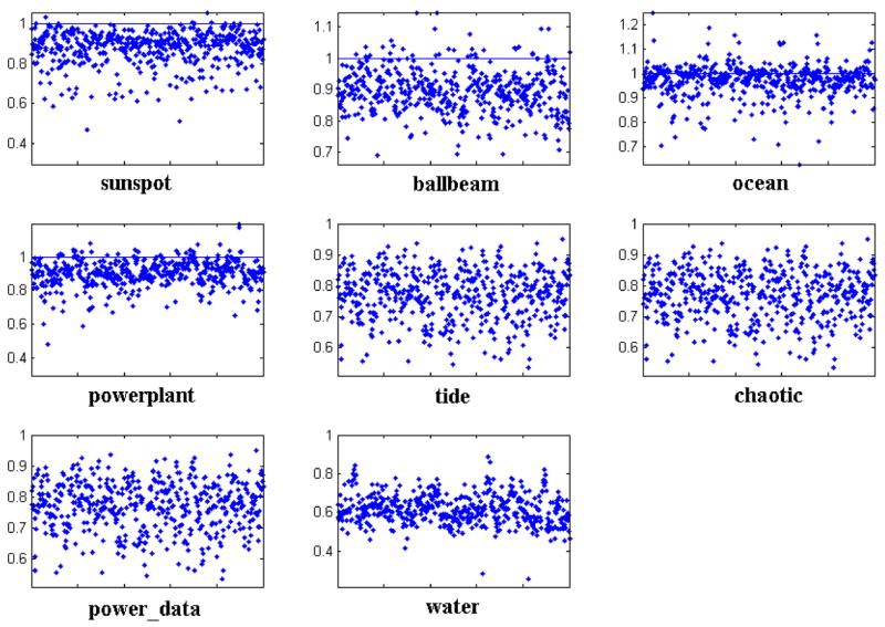
Distribution of the tightness values for PVQA on eight datasets.

In real applications, it is possible that a query Q may contain “outlier” segments which lie far from any samples used for training the codebook. In order to test the ability of PVQA to deal with this situation, we repeated experiments of approximation tightness with the eight datasets where only a randomly selected subset of the data was used for codebook training and the remaining dataset was used for testing. To reach a reliable conclusion, we ran the experiment 50 times with each setting; the average value is reported in Table 3. It is interesting to note that the tightness value for each dataset stays relatively stable while the ratio between training and testing data changes. Except for one dataset (water), all the tightness values are close to 1.

Table 3.

Tightness of approximation values for PVQA when varying the percentage of data used for training and testing.

Percentage of data used for training and testing	70/30%	80/20%	90/10%	96/4%	98/2%
sunspot	1.07	1.06	1.06	1.07	1.06
ballbeam	1.02	1.05	1.05	1.06	1.04
ocean	1.04	1.01	1.00	1.01	1.00
powerplant	1.06	1.06	1.06	1.06	1.06
tide	1.12	1.13	1.13	1.12	1.13
chaotic	1.03	1.06	1.06	1.06	1.07
power_data	1.06	1.03	1.03	1.02	1.02
water	1.25	1.23	1.23	1.23	1.23

4.2 Best Match Searching

Many time series applications involve best match searching. That is, given a query sequence, one must find the best k matches in the database (i.e., having the lowest dissimilarity to the query) or find all the time series whose dissimilarity to the query is below some predefined threshold. In our experiments, we focus on the former, or best k matches. In order to evaluate the performance of different approaches in best match searching, we need an evaluation metric:

Definition 5

For a given query, the set of time series that fall in the same class (based on prior knowledge) is taken as the standard set, and the time series found by different approaches are compared to this set. The matching accuracy, α, is defined as:

$$a=\frac{\mid \mathit{knn}(q)\cap \mathit{std}\_\mathit{set}(q)\mid }{k}\times 100\%$$

In the definition above, knn(q), is the set of k nearest neighbors of the query found by a certain method, while std_set(q) is the standard set (ground truth) which is known in advance. In our experiments, each query’s best k matches (k nearest neighbors) are sought within the database using different approaches and the corresponding accuracies (α) are calculated based on the matching results. We have experimented with various k values for k; the maximum value for k is the actual number of time series within the same class.

In order to increase the reliability of the experiments, the cross-validation technique is applied: the dataset is randomly divided into 5 equal parts and at each time one part is taken as the test (query) set and the rest as the training set. The process is repeated five times and the average results are reported.

• Searching a synthetic dataset

We conducted similarity search experiments on the Control Chart dataset. This dataset contains 600 control charts (each having 60 points) synthetically generated by the process in Alcock and Manolopoulos [31]. The time series belong to six different classes of control charts: Normal, Cyclic, Increasing trend, Decreasing trend, Upward shift, and Downward shift. Each class has 100 time series.

In order to do a thorough comparison, we used different values of k in our experiments. These values range from 10 to 80. For all tested approaches except for the plain Euclidean, we set w = 6 and for PVQA and SAX we set s = 16. Fig. 7 shows the matching accuracy for different approaches. PVQA has the best overall performance. With PVQA, while the outline of the original time series is kept, noise that may affect the calculation of similarities between different time series is removed, and this leads to improved accuracy. However, when k increases, the performance of all three dimensionality reduction approaches (PCA, SAX and PVQA) decreases; they have nearly the same accuracy when k = 80 (i.e., the number of time series from the same class used for training).

Fig. 7.

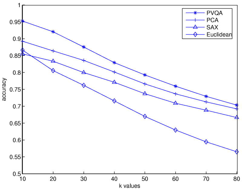
Matching accuracy results for the Control Chart dataset.

• Searching a real dataset

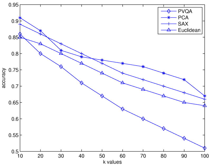
For experiments on real data, we used a dataset of electroencephalographic (EEG) time series. These time series are surface EEG recordings from healthy volunteers with eyes closed and eyes open [32]. Each of the two classes has 100 time series with length n = 4000. We set w = 20 and s = 16 and the values of k ranged from 5 to 80. As shown in Fig. 8, PVQA has the best overall performance while the performance of the other methods drops quickly with the increase of k. The Euclidean has the best behavior for small values of k but then its performance drops quickly below that of the other methods.

Fig. 8.

Matching results for EEG data.

4.3 Clustering time series

We conducted time series clustering experiments on both synthetic and real datasets. We used the PAM (partitioning around medoids) [33] algorithm to cluster the original time-series in every dataset, and applied different approaches for distance calculation that provided different clustering results.

In order to evaluate different approaches, a cluster similarity metric was used. Given two groups of clusters G = G₁,G₂,…,G_K (the true clusters), and A = A₁,A₂,…A_k (clustering result achieved with a certain method), the quality of the clustering was evaluated using the cluster similarity between G and A defined as

$$\mathit{Sim}(G,A)=\frac{{\sum }_i{max}_{\text{j}}\mathit{Sim}(G_i,A_j)}{k}\hspace{0.17em}\text{where\hspace{0.17em}}\hspace{0.17em}\hspace{0.17em}\mathit{Sim}(G_i,A_j)=\frac{2\mid G_i\cap A_j\mid }{\mid G_i\mid +\mid A_j\mid }$$

More details about this metric can be found in [34].

• Clustering a synthetic dataset

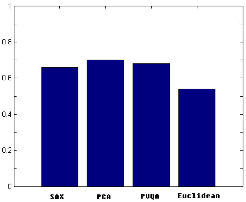
Here, we present the results of the clustering experiments performed on the Control Chart dataset. Since the clustering achieved by PAM depends on the initial choice of medoids, for every dimensionality reduction approach (PCA, SAX, PVQA) and for the Euclidean distance on the original time series (Euclidean), we repeated the clustering process ten times and reported the average accuracy. The values of w and s were set the same as in the best match searching experiments. Fig. 9 shows the results. The clustering performance of the plain Euclidean method is not very good, implying that this distance is not appropriate for providing inter-class dissimilarities for this dataset. The clustering performance of all three piecewise dimensionality reduction techniques (SAX, PCA and PVQA) is comparable and overall much better than that of the plain Euclidean. These results are consistent with those of the similarity search experiments. As shown in Fig. 8, when k = 80, the performance of SAX, PCA and PVQA is very similar.

Fig. 9.

Clustering results for synthetic Control Chart dataset.

These results indicate another advantage of the piecewise approximation techniques. In cases where the Euclidean distance is not appropriate for the distance calculation on the original data (possibly due to the shift along a time axis), piecewise approximation techniques can provide a more meaningful distance measure that can be calculated from a smoothed version of the data.

• Clustering a real dataset

To demonstrate the efficiency of the proposed method in clustering, we performed experiments using real datasets. One of the datasets we used is the per capita personal income dataset (downloadable from [35]). This dataset is a collection of time series presenting the personal yearly income of 25 states in the US during the period of 1929–2001. According to the income growth rates, two classes are defined. One consists mainly of the east coast states with a high rate of income growing, and the other consists of mid-western states in which personal income grows at a slower rate. In our experiments we set w = 6 and s = 16. Fig. 10 demonstrates that PVQA achieves the best clustering results along with plain Euclidean distance that does not perform any dimensionality reduction. The good performance of PVQA is due to the following: since the plain Euclidean method performs very well, the better the approximation we can have with a reduced dimensionality, the better the results that can be achieved.

Fig. 10.

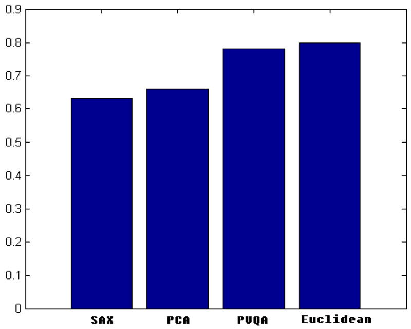
Clustering results for Income dataset.

4.4 Experiments with the LCSS distance measure

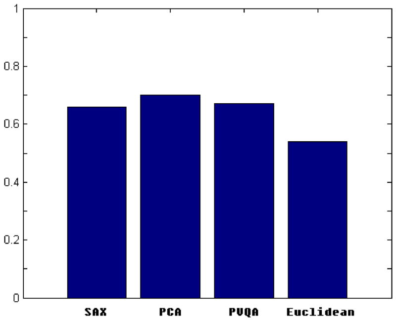
To test the performance of PVQA when used with the LCSS distance measure, we repeated the experiments with this new measure and compared the results to those of other approaches. Here we only list the clustering and retrieval results on the Control Chart dataset.

As shown in Fig. 11, in both clustering and matching experiments, PVQA achieved similar or better classification accuracy to that of PCA, SAX and Euclidean. In both cases, plain Euclidean provides the worst results. The existence of noise and shift on time axis make Euclidean distance not the best choice for this data when calculating the dissimilarity among different time series. With the LCSS measure, PVQA can effectively measure the similarity based on the number of similar subsequences and avoid the effect of noise. This results in better performance.

Fig. 11.

(a) Matching and (b) clustering results for the Control Chart dataset.

4.5 Experiments with text-based similarity measure

We also performed experiments to check the effectiveness of PVQA with a text-based similarity measure (based on the tf-idf profile). The clustering accuracy we obtained on the Control Chart dataset was 0.58. Comparing with the results shown earlier, this accuracy falls between that of plain Euclidean and those of the other methods. The small number of codewords (s = 16) and short length of encoded time series (w = 6) are two of the major reasons that have caused this result. In many text mining applications where tf-idf-based measurements have been applied, there is usually a huge corpus of documents and each document contains at least hundreds or thousands of words. We expect this tf-idf profile measure to be more successful in applications with much larger time series databases. In future work we will investigate this further.

5. DISSCUSSION AND CONCLUSIONS

We have proposed a novel symbolic representation of time series that effectively reduces the dimensionality and improves the efficiency of calculations in clustering and similarity searches. The proposed PVQA approach is a natural extension of the piecewise constant approximation methods that have been previously proposed. By exploiting prior knowledge about the data and allowing the use of a very tight approximation of the Euclidean distance we were able to improve performance in time series analysis over previous state-of-the-art methods.

PVQA partitions a sequence into equal length segments and uses vector quantization to represent each segment by the closest (based on a distance measure) codeword or key-sequence from a codebook. The encoded representation effectively reduces the dimensionality. Experiments we performed on several real and simulated data sets to demonstrate the utility and efficiency of PVQA show that it generally compares favorably to previously proposed dimensionality reduction techniques based on piecewise approximation such as PCA and SAX. The actual results are dataset dependent. Besides good performance, PVQA also has excellent interpretability since it represents a time series using a symbolic representation where the symbols are key-sequences.

The proposed symbolic representation potentially allows for the application of text-based retrieval techniques into the similarity analysis of time series. The RoughDist distance we introduce, provides a very tight approximation to the Euclidean distance defined on the original time series. By allowing the possible existence of a few false dismissals, PVQA reduces the false alarms to a greater extent than other methods. This is potentially very useful for approximate searches. For cases where false dismissals are not acceptable, we propose a modified distance measure that lower bounds the corresponding distance measures defined on the original data. Given the symbolic nature of the proposed time series representation, we also propose a LCSS distance measure and another measure based on tf-idf profiles. These distance measures can be utilized when Euclidean distance is not a viable choice. While the work presented here focuses mainly on similarity analysis of ordered sequences, our approach can also easily be applied to other situations, such as frequent pattern retrieval (i.e., motif discovery), association rule mining, and others.

Directions in which our work can be extended follow below. Based on the application domain, the codewords of the codebook may have real meanings and the importance of different codewords may vary. For example, in stock analysis, we may be more interested in either short term or long term trends. Under such circumstances, different weights should be assigned to the codewords, bringing greater accuracy to similarity retrieval. The best distance measure may depend on the dataset, the task and be user specific; in some cases it can change as the user interactively explores the database [11]. The proposed method can also be extended to represent sequences at different resolutions. Some preliminary results of using multiple codebooks each having codewords of different length have been reported [36]. Future work includes a theoretical study of this relationship. Finally, as Agrawal et al [6] proposed, two time series could be considered similar if they have enough non-overlapping time-ordered pairs of subsequences that are similar. In this case, instead of calculating the dissimilarity using the Euclidean distance, one can introduce the use of histograms to count the frequency of appearance of certain codewords. For example, when comparing two stocks during a long period, we may want to discover during how many months the stocks have similar movements, though the same trend may appear in different months for different stocks. This application is similar to mining motifs in massive time series databases [13].

APPENDIX

Definition 6

Lower bounding rough distance: for two time series X and Q, whose PVQA encoding representation is X′ = x′₁,x′₂,…x′_w and Q′ = q′₁,q′₂,…q′_w, respectively, their lower bounding rough distance is defined as:

$$\text{LB}\_\text{RoughDist}(X,\text{Q})=\sqrt{\sum _{i=1}^w{(d_{x_i^{\prime }{q}_i^{\prime }}^{\prime })}^2}$$

In order to calculate LB_RoughDist, we use a different definition for the distance between each pair of codewords (elements in dist_matrix). Instead of using the Euclidean distance between two codewords c_i and c_j, the minimum distance between their partitions is calculated and stored:

$${d^{\prime }}_{ij}=d_{ij}-r_i-r_j$$

In the equation, r_i and r_j are the radii of the two partitions and d_ij is the Euclidean distance between c_i and c_j. As shown in Fig. 12, the new distance d’_ij defined for the two partitions lower bounds the distance between any pair of the instances in the two partitions. The LB_RoughDist calculated with the modified dist_matrix satisfies the lower bounding condition and guarantees no false dismissals. The proof is straightforward and we show it briefly as follows.

Fig. 12.

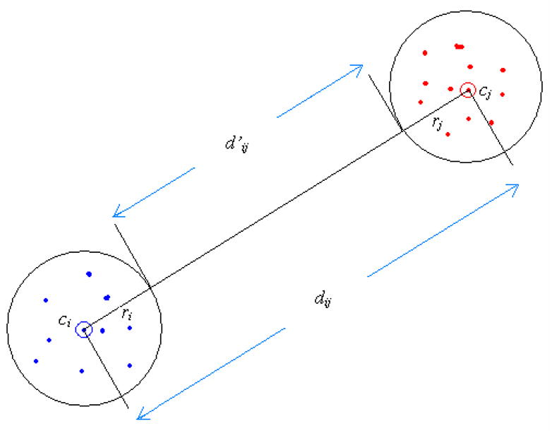
Distance between codewords for the calculation of LB_RoughDist.

Proposition

For any two time series X and Q, whose PVQA representation is X′ = x′₁,x′₂,…x′_w and Q′ = q′₁,q′₂,…q′_w,, respectively, the following inequality between their lower bounding rough distance and Euclidean distance holds:

$$\text{LB}\_\text{RoughDist}(X,\text{Q})\le D(X,Q)$$

Proof

Observe that the right side is

$$D(X,Q)=\sqrt{\sum _{\text{j}=1}^n{(x_j-q_j)}^2}=\sqrt{\sum _{\text{i}=1}^w{(D(x_i^{\prime }-q_i^{\prime }))}^2}$$

and the left side is

$$\text{LB}―\text{RoughDist}(X,\text{Q})=\sqrt{\sum _{i=1}^w{(d_{x_i^{\prime }{q}_i^{\prime }}^{\prime })}^2}.$$

We only need to show that for each i (1 ≤ i ≤ w):

$$d_{x_i^{\prime }{q}_i^{\prime }}^{\prime }\le D(x_i^{\prime }-q_i^{\prime })$$ (1)

Based on the definition of d′, $d_{x_i^{\prime }{q}_i^{\prime }}^{\prime }$ is the minimum distance between two points falling in the partitions represented by codewords $c_{x_i^{\prime }}$ and $c_{q_i^{\prime }}$ respectively. So inequality (1) is true and we have proved that the proposition holds.

References

- 1.Hetland ML. A survey of recent methods for efficient retrieval of similar time sequences, in Data Mining in Time Series Databases. World Scientific; 2002. [Google Scholar]
- 2.Keogh E, Chakrabarti K, Pazzani M, Mehrotra S. Locally adaptive dimensionality reduction for indexinglarge time series databases; Proc. of ACM SIGMOD Conf. on Management of Data; Santa Barbara, CA. 2001. [Google Scholar]
- 3.Survey of Time Series. http://www.cse.cuhk.edu.hk/~mzhou/timeseriesreading.htm.
- 4.Keogh E, Folias T. The UCR time series data mining archive. 2002. [Google Scholar]
- 5.Agrawal R, Faloutsos C, Swami A. Efficient similarity search in sequence databases; Proc. of the 4th Int’l Conf. on Foundations of Data Organization and Algorithms (FODO) Conference; 1993; Evanston, Illinois. [Google Scholar]
- 6.Agrawal R, Lin KI, Sawhney HS, Shim K. Fast imilarity search in the presence of noise, scaling, and translation in time-series databases; Proc. of the 21st Int’l Conf. on Very Large Databases; 1995; Zurich, Switzerland. [Google Scholar]
- 7.Baeza-Yates RA, Gonnet G. A fast algorithm on average for all-against-all sequence matching. Proc. of the String Processing and Information Retrieval Symposium; 1999. [Google Scholar]
- 8.Faloutsos C, Jagadish HV, Mendelzon A, Milo T. A signature technique for similarity-based queries. Proc. of the ACM SIGMOD In’t Conf. on Management of Data; 1997; Positano-salerno, Italy. [Google Scholar]
- 9.Faloutsos C, Equitz W, Flickner M, Niblack W, Petkovic D, Barber R. Efficient and effective querying by image content. Journal of Intelligent Information Systems. 1994;3:231–262. [Google Scholar]
- 10.Huhtala Y, Karkkainen J, Toivonen H. Mining for similarities in aligned time series using wavelets. Data Mining and Knowledge Discovery: Theory, Tools, and Technology, SPIE Proc. Series; 1999; Orlando, FL. [Google Scholar]
- 11.Keogh E, Chakrabarti K, Pazzani M, Mehrotra S. Dimensionality reduction for fast similarity search in large time series databases. Journal of Knowledge and Information Systems. 2000;3(3):263–286. [Google Scholar]
- 12.Keogh E, Pazzani M. An enhanced representation of time series which allows fast and accurate classification, clustering and relevance feedback. Proc. of the 4th Int’l Conf. on Knowledge and Discovery and Data Mining; 1998; New York, NY. [Google Scholar]
- 13.Lin J, Keogh E, Patel P, Lonardi S. Finding motifs in time series; Proc. of the 2nd Workshop on Temporal Data Mining, at the 8th ACM SIGMOD Int’l Conf. on Knowledge Discovery and Data Mining; 2002; Edmonton, Alberta, Canada. [Google Scholar]
- 14.Perng C-S, Wang H, Zhang SR, Parker DS. Landmarks: a new model for similarity-based pattern querying in time series databases; Proc. of the Int’l Conf. on Data Engineering; 2000; San Diego, CA. [Google Scholar]
- 15.Yi B-K, Faloutsos C. Fast time sequence indexing for arbitrary Lp Norms; Proc. of Int’l Conf. on Very Large Data bases; 2000; Cairo, Egypt. [Google Scholar]
- 16.Guttman A. R-trees: a dynamic index structure for spatial searching; Proc. of the ACM SIGMOD; 1984; Boston, MA. [Google Scholar]
- 17.Gusfield D. Algorithms on Strings, Trees and Sequences: Computer Science and Computational Biology. New York: Cambridge Universtiy Press; 1997. [Google Scholar]
- 18.Park S, Chu WW, Yoon J, Hsu C. Efficient search for similar subsequences of different lengths in sequence databases; Proc. of the Int’l Conf. on Data Engineering; 2000; San Diego, CA. [Google Scholar]
- 19.Lin J, Keogh E, Lonardi S, Chiu B. A symbolic representation of time series, with implications for streaming algorithms. Proc. of the 8th ACM workshop on Research Issues in Data Mining and Knowledge Discovery; 2003; San Diego, CA. [Google Scholar]
- 20.Megalooikonomou V, Li G, Wang Q. A Dimensionality Reduction Technique for Efficient Similarity Analysis of Time Series Databases; Proc. of the 13th ACM Conference on Information and Knowledge Management; 2004; Washington, D. C.. [Google Scholar]
- 21.Gersho A, Gray RM. Vector Quantization and Signal Compression. Boston, MA: Kluwer Academic Publishers; 1992. [Google Scholar]
- 22.Linaker F, Niklasson L. Time series segmentation using an adaptive resource allocating vector quantization network based on change detection. Proceedings of the International Joint Conference on Nerual Networks; 2000; Como, Italy. [Google Scholar]
- 23.Lendasse A, Francois D, Wertz V, Verleysen M. Vector quantization: a weighted version for time-series forecasting. Future Generation Computer Systems. 2005;21(7):1056–1067. [Google Scholar]
- 24.Linde S, Buzo A, Gray A. An algorithm for vector quantizer design. IEEE Transactions on Communications. 1980;28:84–95. [Google Scholar]
- 25.Lloyd SP. Least squares quantization in PCM. IEEE Transactions on Information Theory. 1982;IT(28):127–135. [Google Scholar]
- 26.UCI KDD Archive. http://kdd.ics.uci.edu.
- 27.Fowler JE. Adaptive Vector Quantization---Part I: A Unifying Structure; Proceedings of the IEEE Data Compression Conference; 1997; Snowbird, UT. [Google Scholar]
- 28.Vlachos M, Kollios G, Gunopulos G. Discovering similar multidimensional trajectories; Proc. of the 18th Int’l Conf. on Data Engineering; 2002; San Jose, CA. [Google Scholar]
- 29.Salton G, Buckley C. Term-weighting approaches in automatic text retrieval. Information Processing & Management. 1988;24(5):513–523. [Google Scholar]
- 30.Goldin DQ, Kanellakis PC. On similarity queries for time-Series data: constraint specification and implementation; Proc. of the 1st Int’l Conf. on Principles and Practice of Constraint Programming; 1995; Cassis, France. [Google Scholar]
- 31.Alcock RJ, Manolopoulos Y. Time-series similarity queries employing a feature-based approach; Proc. of the 7th Hellenic Conf. on Informatics; 1999; Ioannina, Greece. [Google Scholar]
- 32.Andrzejak RG, Lehnertz K, Rieke C, Mormann F, David P, Elger CE. Indications of nonlinear deterministic and finite dimensional structures in time series of brain electrical activity: Dependence on recording region and brain state. Phys Review E. 2001;64:061907. doi: 10.1103/PhysRevE.64.061907. [DOI] [PubMed] [Google Scholar]
- 33.Kaufman L, Rousseeuw PJ. Finding groups in data: an introduction to cluster analysis. John Wiley & Sons; 1990. [Google Scholar]
- 34.Gavrilov M, Anguelov D, Indyk P, Motwani R. Mining the stock market: which measure is best?; Proc. of the Int’l Conf. on Knowledge Discovery and Data Mining; 2000; Boston, MA. [Google Scholar]
- 35.Regional Accounts Data, Bureau of Economic Analysis. http://www.bea.gov/bea/regional/spi.
- 36.Megalooikonomou V, Wang Q, Li G, Faloutsos C. A Multiresolution Symbolic Representation of Time Series; Proc. of the 21st IEEE International Conference on Data Engineering (ICDE05); 2005; Tokyo, Japan. [Google Scholar]